Sage Journals: Discover world-class research

Abstract

Polarized networks, composed of weakly connected and self-reinforcing groups, can limit the diffusion of ideas, behaviors, and innovations. Here, we use a complex contagion model, in which diffusion depends on both the connectivity and the similarity of individuals, to ask how to optimally build bridges and enhance diffusion in networks characterized by fragmentation and homophily. First, we show that the problem is NP-hard. Then, we explore the space of solutions using heuristics, finding that connecting high degree nodes, or hubs, is an ineffective strategy to accelerate diffusion in fragmented and homophilous networks. We show that in these networks, diffusion is more effectively accelerated by connecting similar but low degree nodes. These results tell us that, in the presence of homophily and polarization, connecting communities through their most central actors may impede rather than facilitate diffusion. Instead, strategies to accelerate the diffusion of innovation, behaviors, and ideas should focus on creating links among the most similar members of different communities. These findings shed light on the diffusion of ideas and innovations in polarized networks.

CCS Concepts: • Mathematics of computing → Network optimization; • Information systems → Social networks

Keywords

homophily polarization social networks social diffusion

Significance statement

Filter bubbles can significantly inhibit the diffusion of ideas and behaviors, motivating the need to explore mechanisms to improve the flow of information among disconnected groups. Here, we explore how to connect dissimilar groups by strategically building bridges that maximize the diffusion of information. Our models assumes diffusion depends on the similarity among individuals (e.g., similarity in attributes that could be thought of as age, gender, tastes, etc.) and on the fraction of an individual’s neighbors who have previously adopted the idea, behavior, or technology. We find that the best strategies involve connecting similar but low-degree nodes. We also find that hubs are effective at promoting diffusion among their groups, but are ineffective as bridges between communities. These findings shed light on the diffusion of ideas and innovations in polarized social networks and suggest that efforts to bridge communities could focus on building relationships among relatively similar individuals from different groups.

Introduction

The diffusion of innovations, behaviors, and ideas is limited by the structure of networks (Pastor-Satorras and Vespignani 2001), the asymmetry of relationships (Christakis and Fowler, 2007), and by homophily (Alshamsi et al., 2015; Bisgin et al., 2010; Christakis and Fowler 2009; McPherson et al., 2001)—the tendency of people to connect with those to whom they are similar. During the last decades, an important area of study in network science has focused on understanding the diffusion of ideas, behaviors, opinions, and diseases, not in idealized networks, but in networks characterized by intricate structures (Barabási and Albert, 1999; Boguá et al., 2003; Dezso and Barabasi, 2001; Kempe et al., 2005; Pastor-Satorras and Vespignani, 2001), tightly knit communities (Stegehuis et al., 2016; Watts and Strogatz, 1998), different spreading dynamics (Pastor-Satorras et al., 2015), asymmetric relationships (Fowler and Christakis, 2008), high degrees of homophily (Raasch et al., 2013), and differential susceptibility (Smilkov et al., 2014).

One area of particular interest is the diffusion of information in homophilous networks. Homophily can hinder the spread of information when people fail to pass on or absorb knowledge from those who are dissimilar (Raasch et al., 2013). Homophily can lead to the formation of echo chambers and redundant information (Lobel and Sadler 2015), limiting our collective ability to adopt behaviors (Rostila, 2010), ideas, and innovations (Burt, 2009; Mäkelä et al., 2012; Rogers 2010; Tortoriello et al., 2012). A key question in this literature is how to promote the diffusion of ideas, innovations, and behaviors, in networks fragmented into homophilous, self-reinforcing communities.

Here, we explore strategies to build bridges among dissimilar communities with the goal to accelerate the diffusion of information. We do this through mathematical modeling and numerical simulations designed to help understand the balance between the roles of homophily and connectivity in accelerating, or impeding diffusion. Our model assumes that pairs of nodes sharing some attributes (e.g., similar in terms age, income, gender, race, occupation, etc.) are more effective at communicating ideas, behaviors, and information, among them, than pairs of dissimilar nodes.

In our model, we gradually add bridges among communities by targeting pairs of nodes based on their connectivity or similarity. We perform analysis for two diffusion models: the independent cascade (Goldenberg et al., 2001) and the linear threshold (Kempe et al., 2003) model. Our results indicate that, in the presence of homophily, diffusion is facilitated by bridges connecting similar nodes rather that high degree nodes. This expands our understanding of network diffusion, which has long emphasized the fact that hubs facilitate spreading in networks (Dezso and Barabasi, 2001; Pastor-Satorras and Vespignani, 2001). Our findings show that linking similar and low degree nodes can be significantly more effective to promote diffusion among dissimilar communities in situations characterized by similarity mediated diffusion and social reinforcement.

Results

Conceptual framework

A diffusion model is a set of rules governing how nodes affect their neighbors. Diffusion models are used to study the spread of ideas, innovations, diseases, and behaviors (Christakis and Fowler, 2007; Karsai et al., 2014; Pastor-Satorras and Vespignani, 2001; Rogers 2010). In the presence of homophily, diffusion can also depend on the similarity of two nodes, the basic assumption being that nodes are more likely to be influenced by their most similar neighbors.

Here, we model the attributes of each node using a vector of values between 0 and 1. Moreover, we consider two similarity metrics: difference similarity (where the distance between two nodes is the average difference between their attributes) and cosine similarity (the cosine of the angle between the two vectors of attributes). Both difference similarity and cosine similarity take values between 0 and 1. Identical vectors have a similarity of one and uncorrelated vectors have a similarity of zero under both metrics.

We use these similarity metrics in two models of diffusion: independent cascade (Goldenberg et al., 2001; Saito et al., 2008; Wang et al., 2012) and linear threshold (Kempe et al., 2003). The independent cascade model is a proxy for simple diffusion. In this model, each node has a chance to activate each of its inactive neighbors. In our case, that probability depends on the similarity between a node and its neighbor. The linear threshold model is a proxy for complex diffusion. Here, activation depends on the sum of similarities with active neighbors. Activation happens when this sum exceeds an inner threshold (e.g., a peer-pressure model). Technical details of the network notation, similarity measures and diffusion models are provided in the Methods section.

To illustrate the trade-offs involved in building bridges between nodes in dissimilar communities, we present a toy model (Figure 1(a)). This toy model involves a network consisting of two components: community 1, containing only a single node, and community 2 containing a path between three nodes. In this model, each node has two numerical attributes. We fix the first attribute of nodes in community 2 to 1, to ensure a high similarity among them and make the second attribute a function of the variable x. When x = 0, all nodes are identical, but dissimilarity grows together with x.

Figure 1.

(a) Toy network used to illustrate the trade-off between connectivity and similarity in the independent cascade model with homophily. Dashed lines represent links that can be added to the network. (b) Difference similarity between nodes as a function of the value of parameter x. The red color denotes the similarity between the seed node A and the central node B, while the blue color denotes the similarity between the seed node A and a peripheral node C. (c) Expected time needed to activate the entire network as a function of the value of parameter x for the independent cascade model. The red line shows the time needed to activate the entire network after adding a link between the seed node and the central node. The blue line represents the time needed to activate the full network after linking the seed node and one of the peripheral nodes. Lines represent analytical curves, points were computed using Monte Carlo simulations.

Now consider a diffusion process starting in community 1. Our goal is to add a connection between the two communities that minimizes the total time needed to diffuse the active state (e.g., the behavior or idea) to the entire network. In this example, we have two options: connecting the node in community 1 to the center of the target community (its hub), or connecting it to one of the peripheral nodes (which are structurally equivalent).

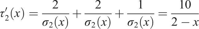
Using the difference similarity metric, the similarity between the seed node in community 1 and the central node of community 2 is σ₁(x) = 1 – x, while the similarity between a peripheral node in community 2 and the seed node or the central node is σ₂(x) = 1 – $\frac{x}{2}$ . Figure 1(b) illustrates how the value of difference similarity between nodes depends on x.

Now we can compute the expected time for activating the entire network after adding an edge between the seed node and the hub of the target community. First, activating the center of the path takes an expected time of $\frac{1}{σ_{1} (x)}$ (since the expected activation time is $τ = \frac{1}{p}$ ). Then, we independently activate both peripheral nodes. Since the probability that in a single round at least one of the peripheral nodes is activated is $1 - (1 - σ_{2} (x))^{2}$ (as $(1 - σ_{2} (x))^{2}$ is the probability that the activation of both nodes fail), it takes on average $\frac{1}{1 - (1 - σ_{2} (x))^{2}}$ rounds until at least one of the peripheral nodes is activated. Let us consider such a situation in which at least one node get activated. With probability σ₂(x)² both peripheral nodes got activated and the additional time necessary to activate the entire network is zero. However, with probability 2σ₂(x) (1 – σ₂(x)) exactly one of the peripheral nodes got activated, in which case we have to wait for the activation of the other peripheral node. Therefore, the conditional probability that we have to wait until the other peripheral node gets activated is $2 σ_{2} (x) (1 - σ_{2} (x)) / 1 - (1 - σ_{2} (x))^{2}$ (the probability that exactly one node got activated divided by the probability that at least one node got activated). If this is the case, we have to wait on average additional $\frac{1}{σ_{2} (x)}$ rounds until the other peripheral node is also activated (the details of these computations are presented in Appendix A). Therefore, the expected time τ₁ for activating entire network is

τ_{1} (x) = \frac{1}{σ_{1} (x)} + \frac{1}{1 - (1 - σ_{2} (x))^{2}} + \frac{2 σ_{2} (x) (1 - σ_{2} (x))}{1 - (1 - σ_{2} (x))^{2}} \frac{1}{σ_{2} (x)} = \frac{1}{1 - x} + \frac{4 (1 + x)}{4 - x^{2}}

Alternatively, if we add an edge between the seed node and one of the peripheral nodes, the expected time needed to independently activate the first peripheral node, followed by the central node, and the remaining peripheral node, is $\frac{1}{σ_{2} (x)}$ . Thus, the total expected time τ₂ to activate the three nodes is equal to

τ_{2} (x) = \frac{1}{σ_{2} (x)} + \frac{1}{σ_{2} (x)} + \frac{1}{σ_{2} (x)} = \frac{6}{2 - x}

Figure 1(c) plots these two functions. We can see that the expected time needed to activate the entire network depends on the value of x. For small values of x, that is when all nodes are similar and the effect of homophily is weak, the structure plays the deciding role. In this case, it is better to connect the seed node to the center of the target community, even though the seed node is more similar to the peripheral nodes. However, for values of x that are greater than $\sqrt{13} - 3 \approx 0.606$ , homophily trumps connectivity. Here, it is optimal to connect the seed node to one of the peripheral nodes. Indeed, for x = 1 the similarity between the seed node and the central node reaches zero. At that point, diffusion can only take place with a connection between the seed node and one of the peripheral nodes (hence, the diverging red line on Figure 1(c)).

Notice that for this network simple heuristics tend to always give the same solution, regardless of the value of x. For example, connecting similar nodes always results in a link between the seed node and a peripheral node, while connecting based on degree always results in a link between the seed node and the central node. Since the optimal choice depends on x, these simple heuristics are inadequate to solve the problem even in this simple case. Nevertheless, heuristics can serve as a good starting point when searching for solutions.

A qualitatively similar result is obtained for the same network in the case of complex diffusion (albeit with a different crossover value for x). Here, we assume that the thresholds are generated using a uniform distribution. If we add an edge between the seed node and the center of the path, the expected time to activate the full network using the linear threshold model is

τ_{1}^{'} (x) = \frac{3}{σ_{1} (x)} + \frac{1}{1 - (1 - σ_{2} (x))^{2}} + \frac{2 σ_{2} (x) (1 - σ_{2} (x))}{1 - (1 - σ_{2} (x))^{2}} \frac{1}{σ_{2} (x)} = \frac{3}{1 - x} + \frac{4 (1 + x)}{4 - x^{2}}

At the same time, if we add an edge between the seed node and one of the peripheral nodes, the expected time to activate the full network using the linear threshold model is equal to

τ_{2}^{'} (x) = \frac{2}{σ_{2} (x)} + \frac{2}{σ_{2} (x)} + \frac{1}{σ_{2} (x)} = \frac{10}{2 - x}

As a result, for values of x that are greater than $\frac{\sqrt{37} - 5}{3} \approx 0.361$ , it is optimal to connect the seed node to one of the peripheral nodes, otherwise it is optimal to connect it to the central node. In Appendix A, we analyze this example in more detail. We also present other illustrative instances of the problem.

Computational complexity of the problem

We now investigate whether it is possible to find an optimal way of building a bridge between two dissimilar communities in a social network. We consider a diffusion process starting from a particular group of nodes called the seed community, that is at the beginning of the process only nodes from the seed community are active. We start with formally defining the problem faced by the party tasked with improving the speed of diffusion.

Definition 2.1

(Forming Bridges). The problem is defined by a tuple $(G, X, \hat{C}, \hat{A}, b, σ, τ)$ , where G = (V, E) is a network, $X \in X^{n}$ is a set of characteristics of the nodes, $\hat{C} \subset V$ is the seed community, $\hat{A} \subseteq \bar{E}$ is the set of edges allowed to be added, $b \in N$ is the budget specifying the maximal number of edges that can be added to the network, σ is a chosen similarity measure, and τ is the function measuring the expected time of activation of an entire network according to a chosen influence model. The goal is then to identify a set of edges $A^{*} \subseteq \hat{A}$ such that A* is in:

{argmin}_{A \subseteq \hat{A} : | A | \leq b} τ ((V, E \cup A), \hat{C})

A trivial solution could be fully to fully connect the two communities. However, this could be either expensive or impossible. Some edges can be too costly to maintain, especially between highly dissimilar people. Other connections may be impossible to create, for example, if prejudice or personal conflict prevents forming a link between two people. To model these kinds of constraints, we introduce set $\hat{A}$ . What is more, there is a suggested cognitive constraint to the number of social relationships that each person can maintain (Hill and Dunbar, 2003). Therefore, the process of adding a number of edges between communities need to be strategic where each new edge is carefully selected to maximize diffusion and accordingly minimize the expected time necessary to activate an entire network.

We investigate the computational complexity of the problem, that is, we ask whether there exists an efficient algorithm of selecting the best edges to be added to a network in order to boost the diffusion between communities. Unfortunately, we find the problem to be an exponential task in a general case, that is, there exists no algorithm that finds an optimal solution for large networks in feasible time. Details of the computational complexity analysis of the problem, including the proof of NP-hardness are presented in Appendix B. The NP-hardness proof is based on a reduction from a well-known Set Cover problem, one of Karp’s twenty one NP-complete problems (Karp, 1972). We show a method of building a network that reflects the structure of a given Set Cover problem instance and use this network as an input to the Forming Bridges problem. We then prove that a solution of the constructed Forming Bridges problem instance corresponds to a solution of the given instance of the Set Cover problem. Hence, if the Forming Bridges problem could be solved in polynomial time, it would imply that the Set Cover problem could also be solved in polynomial time.

Simulation results

Given the computational complexity of the model, we explore more intricate network structures using heuristics and simulations. The technical details of our simulations are presented in Appendix C. Here, we present an overview of the simulations and their main results.

We consider networks consisting of two separate components: one representing the seed community and the other representing the target community. The target community is generated using either the Erdős–Rényi model (Erdős and Rényi, 1959) (where every pair of nodes is connected with the same probability), the Watts–Strogatz model (Watts and Strogatz, 1998) (where resulting networks have small-world property), or the Barabási–Albert model (Barabási and Albert, 1999) (where the structure of the network follows an assortative scale-free topology). Similarly, the seed community is generated using either an Erdős–Rényi model, Watts–Strogatz model, or a Barabási–Albert model. Since the structure of the seed community does not introduce any noticeable differences in our results, here, we report the results in which the seed community is generated using the Erdős–Rényi model. The seed community consists of 500 nodes, all of which are active at the beginning of the simulation, while the target community consists of 2000 nodes, all of which are inactive at the beginning of the simulation. In our simulations, we use undirected networks. While directed networks can carry additional information about a node’s status (Ball and Newman, 2013), they require additional assumptions to guarantee that the entire network can be activated by a diffusion process. In particular, the target community in a directed network has to be strongly connected in order to be able to be activated via an arbitrary bridge, and not every directed network structure could be used in our simulations. Hence, we focus on undirected networks, as any such network can be used as the target community.

To model homophily, we assign two attributes to nodes using different distributions. The mean value of the first attribute is 0.2 in the seed community and 0.8 in the target community, while the mean value of the second attribute is 0.8 in the seed community and 0.2 in the target community. Hence, both attributes contribute to the dissimilarity of seed and target community. We use normal distributions with a standard deviation of 0.05. Results for varying levels of homophily are presented in Appendix D.

Here we build a bridge between two communities using 10 edges. To characterize possible bridge building strategies, we use two key characteristics of the edges: (1) the similarity between the ends of the edge and (2) the average degree of the nodes in an edge. In particular, we consider a strategic space with coordinates

(\frac{k (x) + k (y)}{k_{1}^{*} + k_{2}^{*}}, \frac{σ (x, y)}{σ^{*}})

where k(x) is the degree of node x,

k_{1}^{*}

and

k_{2}^{*}

are the highest and the second highest degree in the network, respectively, σ(x, y) is the similarity between nodes x and y, and σ* is the highest similarity among all pair of nodes in the network. Therefore, every potential edge to be added is translated to a point in this strategic space. Whenever an edge will be added to the network, the heuristic picks the edge closest to a point in the strategic space according to the Euclidean metric. For instance, the (1, 1) strategy will pick edges with the highest average degree and highest similarity, while the

(0, \frac{1}{2})

strategy will pick edges with the lowest average degree and a medium similarity. Notice that this definition of the strategic space guarantees that as long as there are any non-edges between communities, new edges will be added to the network as a result of executing the heuristic. It is theoretically possible that there are no available edges to be added in the direct vicinity of a given point in strategy space, in which case the closest (according to the Euclidean metric) option is selected. However, in our simulations both communities start completely disconnected (which results in 10⁶ edges that can be added to the network), providing a wide range of options, out of which we select only 10.

Figure 2 illustrates our main result by presenting the average time needed to activate an entire Barabási–Albert network using our generalized linear threshold diffusion model with cosine similarity. It shows that, on average, the best results (the lowest total diffusion times) are achieved by adding edges between similar low degree nodes in Barabási–Albert networks (strategies located in the upper left corner of the plot). This strategy is clearly superior to adding an edge between high degree and low similarity nodes (strategies located in the lower right of the plot, which take three times more time than the best strategies).

Figure 2.

Schematic of the simulation model explored, using two random networks of 500 and 2000 nodes. The chart on the right shows the total time needed to activate a network as a function of the average degree, and similarity, of the links added among the two communities. The network consists of the Erdős–Rényi seed community with 500 nodes and a Barabási–Albert target community with 2000 nodes. Our generalized linear threshold diffusion model is used with cosine similarity in these simulations. Results are an average of 100 simulation runs, with new network generated for each run.

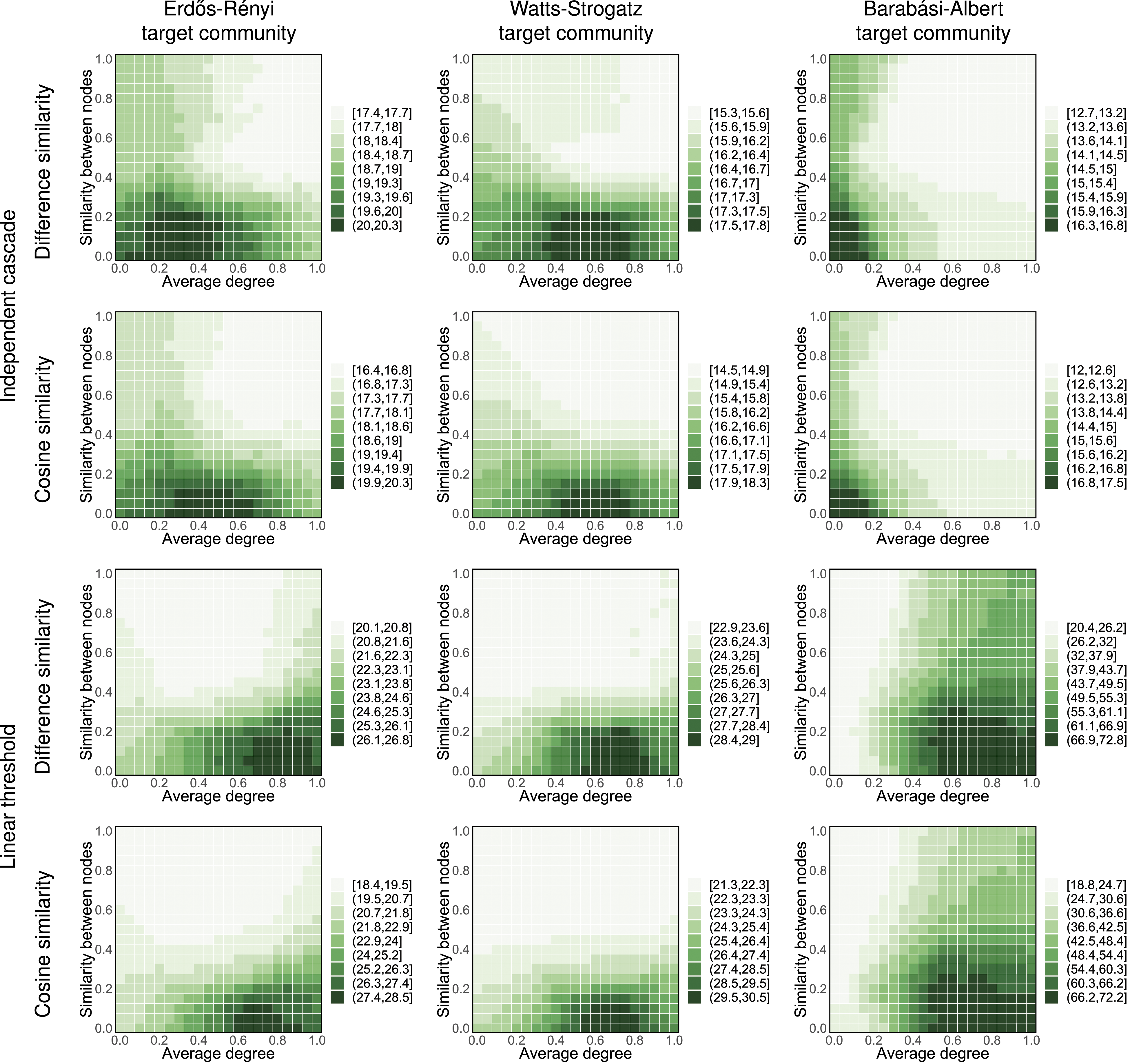
Figure 3 shows this result in more settings, including Erdős–Rényi, Watts–Strogatz, and Barabási–Albert networks, and using simple and complex contagion (respectively independent cascade and linear threshold diffusion models). As expected, heuristics targeting hubs are relatively effective in cases characterized by simple contagion, specially in heterogeneous networks. But when social reinforcement is present (linear threshold diffusion model) adding connections among low degree nodes tends to be a superior strategy, especially if one is able to find low degree nodes that are relatively similar between the source and target community. Even though this result might seem surprising, it is worth noting that in order to spread the diffusion process to the other community, it is first necessary to activate at least one node within it. While a hub may seem like a perfect candidate for such a “foothold,” it can be very difficult to activate, due to suppressing influence from many inactive neighbors and, on average, low similarity with the active neighbors from the source community. On the other hand, if a member of the target community has a low degree, even a single highly similar active neighbor from the source community can significantly sway their opinion. Once at least a few such low-degree members of the target community get activated, they can help the diffusion process reach the hubs, with which they will be on average much more similar than the members of the source community.

Figure 3.

Total time needed to activate a network when using a source community of Erdős–Rényi with 500 nodes and a target community with 2000 nodes. Axes represent the coordinate of the strategic space, with node similarity in the y-axis, and average degree as the x-axis. Color intensity indicates the expected time needed to activate the entire target network. Lower times represent better performance. These results are an average of 100 simulation runs, with new network generated for each run.

Activating the hubs (nodes with highest degrees in the network) is believed to be crucial for spreading diffusion efficiently in social networks (Pastor-Satorras and Vespignani, 2001). However, our results suggest that this is not necessarily the case when similarity and social reinforcement play a role in diffusion process. This is consistent with the literature suggesting that strategic targeting of hubs is not always the most effective diffusion strategy (Alshamsi et al., 2018; Centola and Macy, 2007).

We also perform a number of other experiments, exploring different aspects of our setting. As mentioned above, Appendix D presents our results regarding networks with varying levels of homophily. In general, we find that diffusion is faster in more homophilous networks, but the relative performance of our heuristic strategies remains the same, that is, strategies that are more effective in more homophilous networks tend to be more effective also in less homophilous networks. In Appendix E, we present simulations for networks with varying size of the source and the target community. We find that when it comes to the relative effectiveness of different bridge construction strategies, the observed trends are independent of the network size. In other words, the heuristics that are most effective for a particular diffusion model remain so no matter the size of the network.

Finally, we also consider cases where nodes have differential susceptibility, that is, making some of the nodes less susceptible to activation, which can affect diffusion (Smilkov et al., 2014). To this end, we assume that each node x in the network has a susceptibility coefficient α_x ∈ (0, 1]. To take this coefficient into consideration, we now slightly alter definitions of the diffusion models. In the independent cascade model, the probability of activating node y by its neighbor x is now p (x, y) = α_yσ(x, y)q, where σ is the chosen similarity measure and q is the basic activation probability. In the linear threshold model, an inactive node x becomes active in round t when α_x ∑_{y∈I(t−1)∩N(x)σ(x, y) ≥θx}, where σ is the chosen similarity measure and θ_x is the threshold assigned to the node x. Notice that if for every node we have α_x = 1 then the diffusion model is exactly the same as before. At the beginning of each simulation, we pick pn nodes uniformly at random and we set their susceptibility coefficients to α, where p ∈ [0, 1] and α ∈ (0, 1]. For all other nodes, we set their susceptibility coefficients to 1. We then add 10 edges using the best heuristic from the basic setting and measure the time necessary to activate the entire network.

Our results concerning differential susceptibility are presented in Figure 4. As can be seen from the figure, the value of the susceptibility coefficient of the resilient nodes is considerably more important than the percentage of the population that they constitute. While (Smilkov et al., 2014) reported that even a small group of highly susceptible nodes can support a persisting infection in a Susceptible-Infected-Susceptible model, we analyze an opposite setting and find that even a relatively small number of highly resilient nodes can greatly increase the time necessary to activate a network in our model. At the same time, even a large portion of moderately susceptible nodes has a relatively insignificant effect on the activation time. The results are consistent with respect to the used similarity measure and diffusion model. Our observations confirm that even in a process where diffusion is affected by similarity, differences in individual susceptibility can significantly affect the diffusion dynamics.

Figure 4.

Results for differential susceptibility setting, for the best strategy in each setting. The x-axis of each plot represents the value of α, that is, susceptibility coefficient of the resilient nodes, while the y-axis represents the value of p, that is, the percentage of resilient nodes in the network. Color intensity indicates the expected time needed to activate the entire target network. Lower times represent better performance. These results are an average of 100 simulation runs, with new network generated for each run.

Discussion

Innovations, ideas, and behaviors, can only benefit society if they are able to diffuse. Yet, human society tends to be fragmented, and composed of groups of like-minded people. Homophily is a social glue that on the one hand helps stabilize social groups, but on the other, impedes the diffusion of behaviors, ideas, and innovations among them (Centola 2011; McPherson et al., 2001; Pancs and Vriend 2007; Rogers 2010; Rostila 2010; Singh 2005; Sie et al., 2012; Van de Rijt et al., 2009).

Here, we explored the question of how to accelerate diffusion in networks characterized by homophily and fragmentation. From a computational complexity point of view, we prove the problem to be NP-hard, that is, finding an optimal solution may require exponential computations and is impractical for larger networks. This result highlights the need to approach this problem through heuristic methods that leverage structural information, such as the centrality of nodes, and intrinsic characteristics, such as those explaining the homophily between a pair of individuals. Our results showed that, particularly in the case of the complex contagion, diffusion among dissimilar communities can be accelerated by connecting similar low-degree nodes, instead of connecting dissimilar high-degree nodes. These results are slightly counter-intuitive, given the importance that the network science literature has placed on the connectivity of nodes as a key for diffusion (Dezso and Barabasi, 2001; Pastor-Satorras and Vespignani, 2001. Our findings suggest this to be true only for diffusion based on simple contagion, which in the literature is often associated with modeling phenomena such as contagious diseases (Min and San Miguel, 2018), the spread of rumors (Ibrahim et al., 2016), and viral marketing (Chen et al., 2010). In contrast, complex contagion is usually used to model more intricate processes such as the diffusion of innovations (Karsai et al., 2014), economic diversification and development (Hidalgo et al., 2007; Hidalgo, 2021), participation in social movements (McAdam and Paulsen, 1993), and fashion trends (Crane, 1999). This discrepancy between potential applications of both models gives us a new insight into the interpretation of our findings. The effectiveness of diffusion among the network nodes depends on their absorptive capacity (Cohen and Levinthal, 1990), that is, their ability to assimilate the new information. The spreading of ideas that are relatively easy to internalize can greatly benefit from the involvement of network hubs. However, in the case of ideas that are more difficult to absorb, synergy coming from the similarity between nodes may prove crucial.

It is worth noting that in reality the problem of constructing inter-community bridges might be more complex, as some connections might be more costly, or even impossible to be added, that is, some parts of the strategic space might be inadmissible. A possible way to model such a setting is the use of signed networks (Leskovec et al., 2010), that is, networks in which edges can represent either positive (friendly) or negative (antagonistic) relations. In particular, real-life signed networks are known to exhibit certain structural balance (Kirkley et al., 2019), where some configurations of positive and negative links are preferred over others. It is possible that building bridges that support these preferred configurations might be more beneficial to diffusion in signed networks. Another way in which real-life social networks might be more intricate than those used in our simulations concerns the distribution of node attributes. We assume that said distribution depends solely on the community to which the node belongs. However, a recent study indicates that people with similar network characteristics might share similar neural activity (Baek et al., 2022). It suggests the existence of an additional dimension of homophily, where a hub of community A could be more similar to a hub of community B, than to a low-degree node from community B. If the correlation between the characteristics and behaviors of hubs is systematically strong, and this translates to susceptibility among them, these correlations could make hubs potentially viable bridges. Further research will be needed to understand if that is the case.

Our findings have important lessons and policy implications. While high degree nodes play an important role in network diffusion, they are often hard to influence from outside their own communities. Hubs can therefore be more effective as promoters of diffusion among their own community instead of bridge builders. In fact, linking low-degree but highly similar members of dissimilar communities can give surprisingly good results, suggesting that future efforts to bridge communities could focus on connecting similar members of dissimilar communities. In a world where leaders look for the approval of those who follow them, a better approach to connect opposing groups could be to start from the bottom, by promoting relationships between low connectivity members in their base, and then having that influence percolate up to the leadership.

Methods

Network notation

We denote a network by G = (V, E), where V is a set of n nodes and E ⊆ V × V is a set of edges. We denote the edge between nodes x and y by (x, y). In this work, we consider only undirected networks, that is, networks where E is a set of unordered pairs and we do not discern between edges (x, y) and (y, x). We assume that networks do not contain self-loops, that is, $\forall_{x \in V} (x, x) \notin E$ . By $\bar{E} = V \times V ∖ (\cup_{x \in V} {(x, x)} \cup E)$ we denote the set of all non-existing edges.

We denote the set of neighbors of x in G by N_G(x), that is, $N_{G} (x) = {y \in V : (x, y) \in E}$ . We denote by k_G(x) the number of neighbors (the degree) of a node x, that is, k_G(x) = |N_G(x)|. To make the notation more readable, we will often omit the network itself from the notation, for example, by writing k(x) instead of k_G(x), whenever the network in question is clear from the context.

Similarity measures

To model homophily, that is, the tendency of members of the social network to form ties with people similar to themselves, we need to define properties of each node and measure the similarity between nodes according to these properties. To do this, we assign to each node x a vector of h attributes, that is, vector (x₁, …, x_h). Let $X$ denote the set of all possible attributes vectors. We assume that each attribute has a value from interval [0, 1]. We denote the similarity between two characteristics vectors by $σ : X \times X \to [0,1]$ . We consider the following two similarity measures: difference similarity and cosine similarity.

Difference-similarity is expressed in terms of average difference between attributes values, with all attributes considered equally important

σ_{D} (x, y) = 1 - \frac{\sum_{i} | x_{i} - y_{i} |}{h}

This similarity was used with categorical variables by (Centola, 2011).

Cosine similarity is expressed as the cosine of an angle between two vectors in $R^{h}$ space

σ_{C} (x, y) = \frac{\sum_{i} x_{i} y_{i}}{\sqrt{\sum_{i} x_{i}^{2}} \sqrt{\sum_{i} y_{i}^{2}}}

This similarity was used by (Aral et al., 2009).

Similarity mediated diffusion

We incorporate the similarity measures into two widely used models of diffusion: independent cascade (Goldenberg et al., 2001) and linear threshold (Kempe et al., 2003). Both of these models describe diffusion in a network in terms of node activation. The diffusion process in both models consists of discrete rounds, starting with a small fraction of active “seed” nodes.

In the independent cascade model, each node has a chance to activate each of its inactive neighbors with a constant probability (Goldenberg et al., 2001). The independent cascade model is a proxy for simple diffusion, where diffusion can result from contact with a single “activated” individual (Christakis and Fowler, 2007; Fowler and Christakis, 2008; Pastor-Satorras and Vespignani, 2001; Pastor-Satorras et al., 2015). We assume that the probability of a node activating its inactive neighbor is proportional to the similarity between them, p (x, y) = σ(x, y)q, where p (x, y) is the probability that node x will activate its neighbor y, σ(x, y) is the similarity between the two nodes and q is the basic probability of activation (in our simulations we assume that q = 0.2). Each node tries to activate each of its neighbors in every simulation round.

In the linear threshold model a node becomes active only if a certain fraction of its neighbors are active (Kempe et al., 2003). This model is a proxy for complex diffusion where diffusion requires contact with multiple “active” individuals (Karsai et al., 2014). We implement this model by assuming that the sum of similarities with active neighbors needs to exceed a threshold for a node to be activated (p(x) = P (∑_{y∈A(x)σ(x, y) > θx)} where p(x) is the probability of activating node x, A(x) is the set of active neighbors of x, σ(x, y) is the similarity between nodes x and y, and θ_x is a threshold assigned to node x based on a certain distribution). To guarantee that in the end all nodes in the network are activated, a new threshold is assigned to each inactive node at the beginning of each round (this way in a connected network with non-zero similarities, at least one node always has positive probability of being activated).

Footnotes

Acknowledgments

We acknowledge useful conversations, inspiration, and discussions with Aamena Alshamsi.

Declaration of conflicting interests

The author(s) declared no potential conflicts of interest with respect to the research, authorship, and/or publication of this article.

Funding

The author(s) disclosed receipt of the following financial support for the research, authorship, and/or publication of this article: This work was funded by the Cooperative Agreement between the Masdar Institute of Science and Technology (Masdar Institute), Abu Dhabi, UAE the Massachusetts Institute of Technology (MIT), Cambridge, MA, USA-Reference 02/MI/MIT/CP/11/07633/GEN/G/00. CAH acknowledges support from the Artificial and Natural Intelligence Toulouse Institute - Institut 3iA, ANITI, ANR-19-PI3A-0004.

ORCID iDs

Marcin Waniek

César A Hidalgo

Illustrative examples

To illustrate the model and to demonstrate that homophily can be the driving force behind the diffusion process, we now show some exemplary instances of our problem.

We will first present an example of utilizing simple diffusion, that is, independent cascade model. Consider the network G presented in Figure 1(a) in the main article, consisting of two components, the seed community 1, containing only a single node, and the target community 2 in the form of a path with three nodes. Each node in the network has two numerical attributes, with values depicted in the figure. Attribute values of most of the nodes are determined by the parameter x ∈ [0, 1].

The difference similarity between the node from the seed community and the center of the path is

σ_{1} (x) = 1 - \frac{| x - 0 | + | 1 - x - 1 |}{2} = 1 - x

While the similarity between a peripheral node and either the seed node or the center of the path is

σ_{2} (x) = 1 - \frac{| x - x | + | 1 - (1 - x) |}{2} = 1 - \frac{| x - 0 | + | 1 - 1 |}{2} = 1 - \frac{x}{2}

As it can be seen, for x = 0 the similarity between every two nodes in the network is equal to 1, as for x = 0 all nodes has exactly the same attributes values. While x increases, the similarity between the seed node and the center of the path decreases, until it reaches 0, while the similarity between peripheral nodes and other types of nodes in the network decreases until it reaches 1/2. Figure 1(b) illustrates how the value of difference similarity between nodes depends on the value of x.

Given these similarity values we can compute the expected time of activating entire network after adding an edge between the seed node and either the center of the path or one of the peripheral nodes. If we add an edge between the seed node and the center of the path, the expected time of activation is equal to

τ_{1} (x) = \frac{1}{σ_{1} (x)} + \frac{1 + 2 (1 - σ_{2} (x))}{1 - (1 - σ_{2} (x))^{2}} \frac{1}{σ_{2} (x)} = \frac{1}{1 - x} + \frac{1 + x}{1 - \frac{x^{2}}{4}} = \frac{1}{1 - x} + \frac{4 (1 + x)}{4 - x^{2}}

As first we need to activate the center of the path in expected time $\frac{1}{σ_{1} (x)}$ and then we independently activate both peripheral nodes. It takes on average $\frac{1}{1 - (1 - σ_{2} (x))^{2}}$ rounds until at least one of them is activated. Then, the probability that only one peripheral node became activated is $2 σ_{2} (x) (1 - σ_{2} (x)) / 1 - (1 - σ_{2} (x))^{2}$ (where 2σ₂(x) (1 − σ₂(x)) is the probability that exactly one peripheral becomes activated, while $1 - (1 - σ_{2} (x))^{2}$ is the probability that at least one becomes activated) and we have to wait on average $\frac{1}{σ_{2} (x)}$ rounds until the other peripheral node is also activated.

On the other hand, if we add an edge between the seed node and one of the peripheral nodes, the expected time of activation is equal to

τ_{2} (x) = \frac{1}{σ_{2} (x)} + \frac{1}{σ_{2} (x)} + \frac{1}{σ_{2} (x)} = \frac{3}{1 - \frac{x}{2}} = \frac{6}{2 - x}

As first we need to activate the peripheral that we connect to the seed, then we activate the center of the path, and then we independently activate the remaining peripheral node, each of them in expected time 1/σ₂(x).

Figure 1(c) illustrates how the expected time of activation of the entire network depends on the value of parameter x. We can see that depending on the values of similarity (determined by the value of x) the structure of the network itself becomes more or less important. For the low values of x, that is, when all nodes in the network are highly similar to each other, the structure plays the deciding role and it is the optimal choice to connect the seed node to the center of the path, even though the seed node itself is more similar to the peripheral nodes. We have τ₁(x) = τ₂(x) for $x = \sqrt{13} - 3$ ; hence, for the values of x higher than $\sqrt{13} - 3$ , it is optimal to connect the seed node to one of the peripheral node. Indeed, for x = 1 the similarity between the seed node and the center of the path reaches zero; hence, the diffusion can only take place with a connection between the seed node and one of the peripheral nodes.

Let us now analyze the complex diffusion case for the same network. We will assume that the thresholds are generated using uniform distribution. If we add an edge between the seed node and the center of the path, the expected time of activation under linear threshold model is equal to

τ_{1}^{'} (x) = \frac{3}{σ_{1} (x)} + \frac{1}{1 - (1 - σ_{2} (x))^{2}} + \frac{1 + 2 (1 - σ_{2} (x))}{1 - (1 - σ_{2} (x))^{2}} \frac{1}{σ_{2} (x)} = \frac{3}{1 - x} + \frac{1 + x}{1 - \frac{x^{2}}{4}} = \frac{3}{1 - x} + \frac{4 (1 + x)}{4 - x^{2}}

At the same time, if we add an edge between the seed node and one of the peripheral nodes, the expected time of activation under linear threshold model is equal to

τ_{2}^{'} (x) = \frac{2}{σ_{2} (x)} + \frac{2}{σ_{2} (x)} + \frac{1}{σ_{2} (x)} = \frac{5}{1 - \frac{x}{2}} = \frac{10}{2 - x}

Figure 5 presents the expected time of activating the entire network under linear threshold model. As it can be seen, the general trends are analogical to these of the independent cascade model. Figure 5.

Time of activation of an entire network as a function of the value of parameter x, given the linear threshold model. The red color represents impact of adding an edge between the seed and the center while the blue color represents the impact of adding an edge between the seed and any peripheral node.

We now present another example of a similarity-based diffusion in the presence of complex diffusion in a network, that is, the linear threshold model. Consider a network with two different types of nodes and only one numerical attribute for each node. For the filled nodes, the value of this attribute is 1, while for the empty nodes it is determined by parameter x ∈ (0, 1]. In this network, we have two communities: the seed community C₁ with one filled node and one empty node connected with an edge, as well as community C₂ consisting of k filled nodes and k empty nodes connected into a path. Let us assume that we are only allowed to add an edge between one node from the seed community and one of the ends of the path. The situation is presented in Figure 6. Figure 6.

The network used to illustrate effects of homophily on the expected time of activation in the linear threshold model.

Now let us consider how the expected time of activation of the entire network depends on the order of k filled and k empty nodes in community C₂. Notice that every node v in community C₂ becomes activated when only one of its neighbors active. We will call this neighbor the predecessor, and the other neighbor (if it exists) the successor of v.

Figure 7 presents the expected time of activation of a node under linear threshold model, depending on the types of its predecessor v′ and successor v^″. We will consider various possible orders of empty and filled nodes in community C₂ presented in Figure 8. In particular, Figure 8(a) presents a network with k filled nodes followed by k empty nodes. In the network presented in Figure 8(a), the expected time of activation of the entire network is

τ_{a} (x) = 2 k + \frac{2}{x} + 2 (k - 2) + 1 = 4 k - 3 + \frac{2}{x}

Figure 7.

Expected time of activation of node v depending on the types of its predecessor v′ and successor v^″, given the linear threshold model. Numbers on edges express similarities between nodes.

Figure 8.

Examples of possible orders of empty and filled nodes in community C₂. The network in subfigure (C) gets activated faster than the network in subfigure (B), but slower than the network in subfigure (A).

Since each of the k filled nodes is activated in expected time 2, the first empty node is activated in expected time 2/x, the following k − 2 empty nodes in expected time 2 each, and finally the last node in time 1. Hence, for a totally segregated network the expected time of activation is 4k − 3 + 2/x.

Moving to the network presented in Figure 8(b), its total expected time of activation is

τ_{b} (x) = 2 + (2 k - 2) \frac{2}{x} + \frac{1}{x} = \frac{4 k - 3}{x} + 2

Since the first filled node is activated in expected time 2, the following 2k − 2 nodes are activated in expected time $\frac{2}{x}$ each, while the last node is activated in time $\frac{1}{x}$ . Hence, in such network the total expected time of activation is never shorter than in a fully segregated network.

Finally, for network presented in Figure 8(c) the expected time of activation is

τ_{c} (x) = 2 k + (k - 1) \frac{2}{x} + \frac{1}{x} = \frac{2 k - 1}{x} + 2 k

Since every of the k nodes with predecessor of the same type is activated in expected time 2, k − 1 nodes with predecessors of different types are activated in expected time 2/x each, while the last node is activated in time 1/x. In particular, we have that τ_c is always greater than τ_a and it is always smaller than τ_b. As it can be seen, the most homogenous structure provides the best expected time of activation.

Complexity analysis

Here, we present the proof of NP-hardness of the Forming Bridges problem.

Theorem B.1

Forming Bridges problem is NP-hard for independent cascade and linear threshold diffusion models.

Proof.

The decision version of the optimization problem is the following: given a network G = (V, E), a set of characteristics of the nodes X, the seed community $\hat{C}$ , is the set of edges allowed to be added $\hat{A}$ , the budget b, a similarity measure σ, a function τ measuring the expected time of activation according to a certain influence model, and a value $τ^{*} \in R$ , determine whether there exists a set of edges $A^{*} \subseteq \hat{A}$ such that |A*| ≤ b and $τ ((V, E \cup A^{*}), \hat{C}) \leq τ^{*}$ .

The main idea of the NP-hardness proof is as follows. We will show a reduction from the NP-complete Set Cover problem. We build a network that reflects the structure of a given Set Cover problem instance and use it as an input for the Forming Bridges problem. Finally, we show that a solution of the Forming Bridges problem corresponds to a solution of the given instance of the Set Cover problem.

An instance of the NP-complete Set Cover problem is defined by a universe U = {u₁, …, u_m}, a collection of sets S = {S₁, …, S_k} such that ∀_jS_j ⊂ U, and an integer b ≤ k. The goal is to determine whether there exist b elements of S the union of which equals U.

We will now create a network G based on the given instance of the Set Cover problem, as shown in Figure 9:

• The set of nodes: For every S_i ∈ S, we create a single node, denoted by S_i. For every u_i ∈ U, we create a single node, denoted by u_i. We also create a single node a.

• The set of edges: For every u_j ∈ U and every S_i ∈ S such that u_j ∈ S_i we create an edge (S_i, u_j). Moreover, for every two nodes S_i, S_j ∈ S we create an edge (S_i, S_j), that is, we connect the nodes from set S into a clique.

Let X be a set of characteristics such that every node has only one attribute, and all of them has the same value of the attribute. Notice that in that situation we have that similarity between any two nodes in the network is 1, no matter what the chosen similarity measure is σ.

Let the diffusion model (represented by function τ) be either the independent cascade model with q = 1 or the linear threshold model with distribution of thresholds always returning 1. Notice that under these conditions for both diffusion models we have that every node in the network becomes activated as soon as at least one of its neighbors becomes activated. This is because in the independent cascade model all probabilities of activation are equal to 1 (as similarity between all pairs of nodes is 1), and in the linear threshold model all thresholds are equal to 1.

Moreover, let the seed community be $\hat{C} = {a}$ , the set of edges allowed to be added be $\hat{A} = {(a, S_{i}) : S_{i} \in S}$ , the budget b be the same as in the given Set Cover problem instance, and the expected time in which we intend to activate entire network be τ* = 2.

Now, consider an instance of the problem of Forming Bridges $(G, X, \hat{C}, \hat{A}, b, σ, τ, τ^{*})$ . We will now show that an optimal solution to this instance corresponds to an optimal solution to the given instance of the Set Cover problem.

First, we will show that if there exists a solution to the given instance of the Set Cover problem, there also exists a solution to the constructed instance of the Forming Bridges problem. Let S* be a solution to the given instance of the Set Cover problem. Now, consider a solution to the constructed instance of the Forming Bridges problem A* = {(a, S_i): S_i ∈ S*}. In the network (V, E ∪ A*), all nodes in S* becomes activated in the first activation round. Then, in the second round, all their neighbors become activated. Since S* is a solution to the given instance of the Set Cover problem, for every node u_j there exists a node S_i such that S_i ∈ S* and u_j is connected with S_i. All other nodes S_i ∉S* are neighbors of nodes in S*; hence, they also become activated in the second round. Therefore, the expected time of activation of an entire network is 2 and A* is a solution to the constructed instance of the Forming Bridges problem.

Now, we will show that if there exists a solution to the constructed instance of the Forming Bridges problem, then there also exists a solution to the given instance of the Set Cover problem. Let A* be a solution to the constructed instance of the Forming Bridges problem. Consider a set S* = {S_i ∈ S: (a, S_i) ∈ A*}. We will now show that S* is a solution to the given instance of the Set Cover problem. Consider the activation process in the network (V, E ∪ A*). In the first round, all nodes in S* become activated as these are the only neighbors of node a, the sole member of the seed community. Since A* is a solution to the constructed instance of the Forming Bridges problem, we have $τ ((V, E \cup A), \hat{C}) \leq 2$ ; hence, all the remaining nodes have to become activated in the second round of activation, including all nodes u_j ∈ U. Therefore, for every node u_j ∈ U there must exist a node S_i ∈ S* such that u_j is connected with S_i. Because of the way we constructed the network G, this also means that for every u_j ∈ U there exists a node S_i ∈ S* such that u_j ∈ S_i. Hence, S* is a solution to the given instance of the Set Cover problem.

This implies that the constructed instance of the Forming Bridges problem has a solution if and only if the given instance of the Set Cover problem has a solution, thus concluding the proof.

Experimental analysis of the model

We now present the setting of our experiments using different heuristic techniques of connecting dissimilar communities.

In the basic version of our experiments, we consider a network consisting of two disconnected components, each of them forming a separate community. One of the communities is active from the beginning of the process (the seed community), whereas the other community we will call the target community. Every component of the initially disconnected network is generated using one of the following standard network generation models:

• Random networks generated using the Erdős–Rényi model (Erdős and Rényi, 1959). For every pair of nodes, we add an edge between them with a certain probability. We denote such a network by ER (n, d), where n is the number of nodes and d is the expected average degree.

• Small world networks generated using the Watts–Strogatz model (Watts and Strogatz, 1998). The network starts as a regular ring lattice, and each edge network is then rewired with probability p = 0.25. We denote such a network by WS (n, d), where n is the number of nodes and d is the expected average degree.

• Preferential attachment networks generated using the Barabási–Albert model (Barabási and Albert, 1999). We add nodes to the network one by one. For each node, we create a constant number of new edges, connecting it to nodes added previously with a probability proportional to their degrees. We denote such a network by BA (n, d), where n is the number of nodes and d is the number of links added with each node.

For every node. we generate attribute values based on certain distributions. To reflect the differences between communities, the distribution we use for generating attributes is different for every community. In our experiments, we assume that every node has two different numerical attributes, a1 and a2. All distributions are normal distributions where the value of standard deviation is 0.05. For the seed community, we generate the value of a1 from distribution with mean 0.2 and the value of a2 from distribution with mean 0.8. For the target community, we generate the value of a1 from distribution with mean 0.8 and the value of a2 from distribution with mean 0.2.

In the independent cascade model, we set the basic probability of activation to q = 0.2. In the linear threshold model, we use uniform distribution to choose the value of thresholds. In each of our experiments, we build a bridge consisting of 10 edges. We always pick an edge connecting one node from the seed community and one node from the target community. The results of these experiments are presented in the main article.

In another series of experiments we compare the performance of the best strategy for each network with the following baseline solutions (in all cases ties are broken uniformly at random):

• Max similarity algorithm where we connect two nodes with the highest similarity measure value,

• Min similarity algorithm where we connect two nodes with the lowest similarity measure value,

• Max degree algorithm where we connect two nodes with the highest sum of degrees,

• Min degree algorithm where we connect two nodes with the lowest sum of degrees,

• Random algorithm where we connect a pair of nodes chosen uniformly at random, we use this strategy as a baseline.

Figure 10 presents plots of expected time necessary to activate entire network for different networks, similarity measures and diffusion models. In all cases, the best parametric strategy is among the most effective ways of constructing the bridge between communities. Figure 10.

Comparison between the expected time of activating entire network for the best (for this particular setting) strategy and baseline heuristics, in network consisting of the ER (500, 10) seed community and a target community with 2, 000 nodes. Plots are presented with logarithmic scales. The results are presented as an average over 100 simulation runs, with new network generated for each run. Colored areas represent 95% confidence intervals.

As for the comparison between the independent cascade and linear threshold diffusion models, the main difference is the change of efficiency of the degree-based heuristic algorithms. For the independent cascade model, the max degree heuristic is far more efficient than its min counterpart. This is because connecting to nodes with high degree helps to reach a large number of nodes in the target community in just a single step. As for the linear threshold model, simply connecting to a high degree node that does not already have a large number of neighbors in the seed community, makes this node extremely hard to activate, as one new neighbor has very small contribution to the total sum of similarities necessary to overcome the threshold. On the other hand, a low degree node in a linear threshold model is fairly easy to activate as every new connection accounts for a considerable part of the total sum of similarity with its neighbors.

Experiments with different levels of homophily

We now perform a series of experiments to check how the different levels of homophily affect the effectiveness of various strategies of building bridges between communities. We start with the network where attributes are determined as in the basic experiments, that is, all nodes in the seed community have attributes taken from one distribution, while all nodes in the target community have attributes taken from a different distribution. We call nodes from the seed community type I nodes and we call nodes with the target community type II nodes. We call an edge between a node of type I and a node of type II an inter-type edge.

For such a network we repeatedly perform the following procedure. We change places of two nodes, one of type I and one of type II, such that this change increases the number of inter-type edges in the network. Other than this requirement, the nodes to change places are chosen uniformly at random. We measure the percentage of inter-type edges in the network and the time necessary to activate entire network after building a bridge (consisting of 10 edges) between both communities. The results of our experiments are presented in Figures 11–13 for the strategy space, while Figure 14 presents the changing effectiveness of the best strategy (in a network without inter-type edges) in each setting. Figure 11.

Results for experiments with different levels of homophily, for network consisting of the ER (500, 10) seed community and ER (2000, 10) target community. The segregation value is expressed as the percentage of inter-type edges in the network.

Figure 12.

Results for experiments with different levels of homophily, for network consisting of the ER (500, 10) seed community and WS(2000, 10) target community. The segregation value is expressed as the percentage of inter-type edges in the network.

Figure 13.

Results for experiments with different levels of homophily, for network consisting of the ER (500, 10) seed community and BA (2000, 5) target community. The segregation value is expressed as the percentage of inter-type edges in the network.

Figure 14.

Results of experiments with different homophily levels for best heuristic in network without inter-type edges. Each line represents results for different target community. Colored areas represent 95% confidence intervals. Scales are fixed for easier comparison.

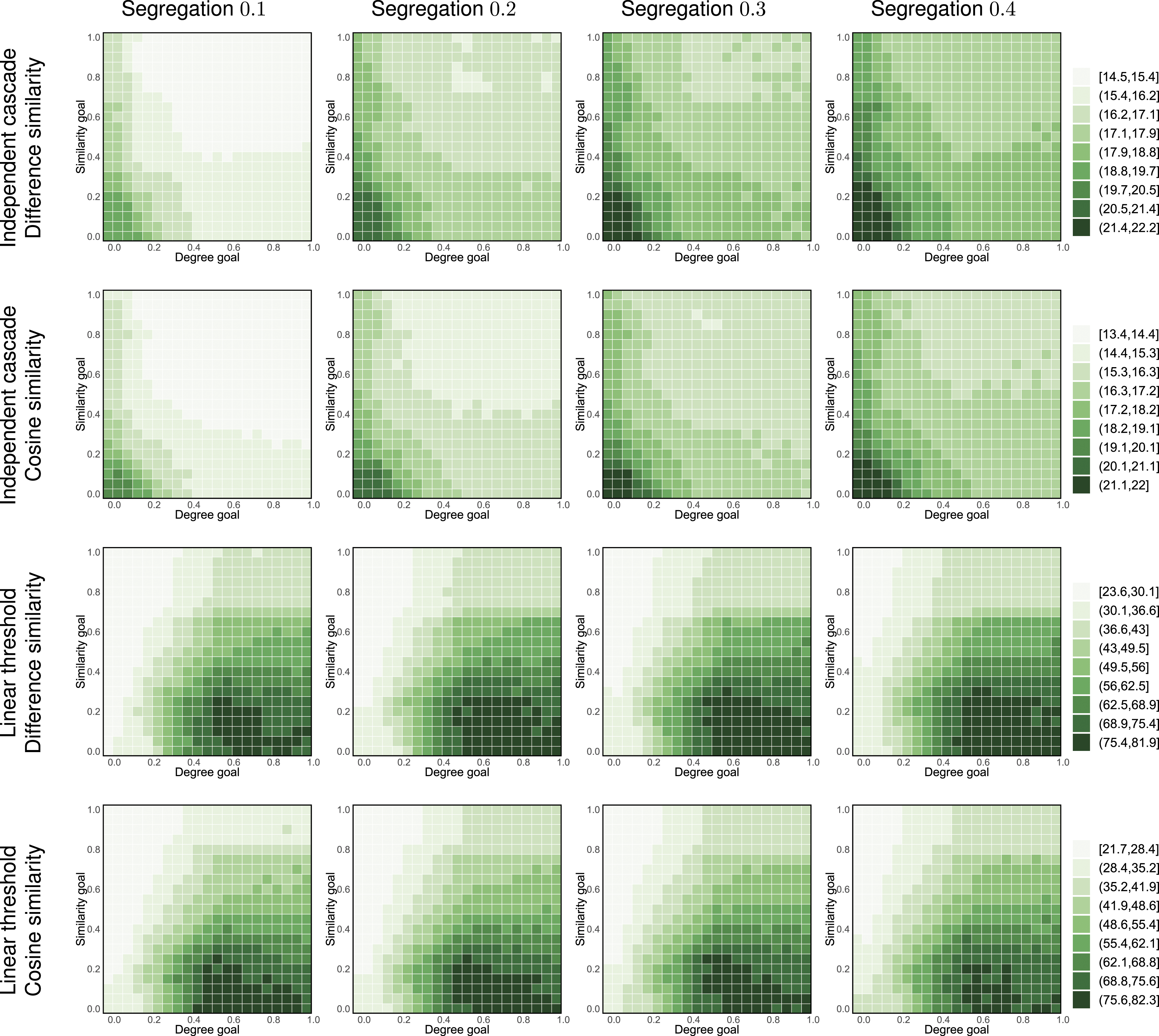
As it can be seen, time necessary to activate the entire network decreases with homophily in case of both independent cascade and linear threshold models. In case of the independent cascade model, higher homophily results in higher average probability of activation (as similarity of two nodes connected with inter-type edge is lower than two nodes of the same type). In case of the linear threshold model, a lower expected similarity on edges decreases the probability of becoming activated, as our swapping procedure keeps degree of each node constant. Moreover, this confirms our observations about the nature of complex contagion in homophilous and heterophilous networks made in Appendix A.

Results for networks with varying size

We now perform a series of experiments investigating the effect of network size on the effectiveness of different ways of constructing a bridge between communities. While in the main article, we focus on networks consisting of a source community with 500 nodes and a target community with 2000 nodes, here we also run simulations for smaller networks.

Figures 15–17 present our results. As can be seen from the figures, the trends observed for smaller networks are the same as those for their larger counterparts presented in Figure 3. It suggests that the findings reported in the main article might be independent on the size of the network. Figure 15.

Same as Figure 3 but for networks consisting of a source community of Erdős–Rényi with 250 nodes and a target community with 1000 nodes.

Figure 16.

Same as Figure 3 but for networks consisting of a source community of Erdős–Rényi with 500 nodes and a target community with 1000 nodes.

Figure 17.

Same as Figure 3 but for networks consisting of a source community of Erdős–Rényi with 250 nodes and a target community with 2000 nodes.

References

Alshamsi

Awad

Almehrezi

, et al. (2015) Misery loves company: happiness and communication in the city. EPJ Data Science 4: 17.

Alshamsi

Pinheiro

Hidalgo

(2018) Optimal diversification strategies in the networks of related products and of related research areas. Nature Communications 9: 11328.

Aral

Muchnik

Sundararajan

(2009) Distinguishing influence-based contagion from homophily-driven diffusion in dynamic networks. Proceedings of the National Academy of Sciences 106: 21544–21549.

Baek

Ryan

López

, et al. (2022) In-degree centrality in a social network is linked to coordinated neural activity. Nature Communications 13: 1118.

Ball

Newman

MEJ

(2013) Friendship networks and social status. Network Science 1: 1–30.

Barabási

A-L

Albert

(1999) Emergence of scaling in random networks. Science 286: 5439–5512.

Bisgin

Agarwal

(2010) Investigating homophily in online social networks. In: Web Intelligence and Intelligent Agent Technology (WI-IAT), 2010 IEEE/WIC/ACM International Conference on Vol. 1, New York, NY: IEEE, pp. 533–536.

Boguá

Pastor-Satorras

Vespignani

(2003) Epidemic spreading in complex networks with degree correlations. In: Statistical Mechanics of Complex Networks. New York, NY: Springer, pp. 127–147.

Burt

(2009) Structural Holes: The Social Structure of Competition. Cambridge, MA: Harvard University Press.

10.

Centola

(2011) An experimental study of homophily in the adoption of health behavior. Science 334: 1269–1272.

11.

Centola

Macy

(2007) Complex contagions and the weakness of long ties. American Journal of Sociology 113(3): 702–734.

12.

Chen

Wang

(2010) Scalable influence maximization for prevalent viral marketing in large-scale social networks. In: Proceedings of the 16th ACM SIGKDD International Conference on Knowledge Discovery and Data Mining. New York, NY: ACM, pp. 1029–1038.

13.

Christakis

Fowler

(2007) The spread of obesity in a large social network over 32 years. New England journal of medicine 357(4): 370–379.

14.

Christakis

Fowler

(2009) Connected: The Surprising Power of Our Social Networks and How They Shape Our Lives. Boston, IL: Little Brown & Co.

15.

Cohen

Levinthal

(1990) Absorptive capacity: a new perspective on learning and innovation. Administrative Science Quarterly 35(1990): 128–152.

16.

Crane

(1999) Diffusion models and fashion: a reassessment. The Annals of the American Academy of Political and Social Science 566: 13–24.

17.

Dezso

Barabasi

A-L

(2001) Can we stop the AIDS epidemic? Physical Review E 65: 055103. cond-mat/0107420.

18.

Erdős

Rényi

(1959) On random graphs I. Publicationes Mathematicae Debrecen 6(1959): 290–297.

19.

Fowler

Christakis

(2008) Dynamic spread of happiness in a large social network: longitudinal analysis over 20 years in the framingham heart study. Bmj: British Medical Journal 337: a2338.

20.

Goldenberg

Libai

Muller

(2001) Using complex systems analysis to advance marketing theory development: modeling heterogeneity effects on new product growth through stochastic cellular automata. Academy of Marketing Science Review 9: 1–19.

21.

Hidalgo

(2021) Economic complexity theory and applications. Nature Reviews Physics 3(2): 92–113.

22.

Hidalgo

Bailey

Barabási

A-L

, et al. (2007) The product space conditions the development of nations. Science 317: 5837–6487.

23.

Hill

Dunbar

RIM

(2003) Social network size in humans. Human Nature 14: 53–72.

24.

Ibrahim

Hefny

Hassanien

(2016) Controlling rumor cascade over social networks. In: International Conference on Advanced Intelligent Systems and Informatics. New York, NY: Springer, pp. 456–466.

25.

Karp

(1972) Reducibility among combinatorial problems. In: Complexity of Computer Computations. New York, NY: Springer, pp. 85–103.

26.

Karsai

Iniguez

Kaski

, et al. (2014) Complex contagion process in spreading of online innovation. Journal of The Royal Society Interface 11(101): 20140694.

27.

Kempe

Kleinberg

Tardos

(2003) Maximizing the spread of influence through a social network. In: Proceedings of the Ninth ACM SIGKDD International Conference on Knowledge Discovery and Data Mining. New York, NY: ACM, pp. 137–146.

28.

Kempe

Kleinberg

Tardos

(2005) Influential nodes in a diffusion model for social networks. In: International Colloquium on Automata, Languages, and Programming. New York, NY: Springer, pp. 1127–1138.

29.

Kirkley

Cantwell

Newman

MEJ

(2019) Balance in signed networks. Physical Review E 99: 012320.

30.

Leskovec

Huttenlocher

Kleinberg

(2010) Signed networks in social media. In: Proceedings of the SIGCHI Conference on Human Factors in Computing Systems. New York, NY: ACM, pp. 1361–1370.

31.

Lobel

Sadler

(2015) Preferences, homophily, and social learning. Operations Research 64(3): 564–584.

32.

Mäkelä

Andersson

Seppälä

(2012) Interpersonal similarity and knowledge sharing within multinational organizations. International Business Review 21(3): 439–451.

33.

McAdam

Paulsen

(1993) Specifying the relationship between social ties and activism. American Journal of Sociology 99(3): 640–667.

34.

McPherson

Smith-Lovin

Cook

(2001) Birds of a feather: homophily in social networks. Annual Review of Sociology 27: 415–444.

35.

Min

San Miguel

(2018) Competing contagion processes: complex contagion triggered by simple contagion. Scientific Reports 8: 10422.

36.

Pancs

Vriend

(2007) Schelling’s spatial proximity model of segregation revisited. Journal of Public Economics 91: 1–24.

37.

Pastor-Satorras

Castellano

Van Mieghem

, et al. (2015) Epidemic processes in complex networks. Reviews of modern physics 87: 3925–3979.

38.

Pastor-Satorras

Vespignani

(2001) Epidemic spreading in scale-free networks. Physical Review Letters 86: 3200–3203.

39.

Raasch

Lee

Spaeth

, et al. (2013) The rise and fall of interdisciplinary research: the case of open source innovation. Research Policy 42: 1138–1151.

40.

Rogers

(2010) Diffusion of Innovations. New York, NY: Simon & Schuster.

41.

Rostila

(2010) Birds of a feather flock together–and fall ill? migrant homophily and health in Sweden. Sociology of Health & Illness 32: 382–399.

42.

Saito

Nakano

Kimura

(2008) Prediction of information diffusion probabilities for independent cascade model. In: International Conference on Knowledge-Based and Intelligent Information and Engineering Systems. New York, NY: Springer, pp. 67–75.

43.

Sie

Drachsler

Bitter-Rijpkema

, et al. (2012) To whom and why should I connect? Co-author recommendation based on powerful and similar peers. International Journal of Technology Enhanced Learning 4: 121–137.

44.

Singh

(2005) Collaborative networks as determinants of knowledge diffusion patterns. Management Science 51(5): 756–770.

45.

Smilkov

Hidalgo

Kocarev

(2014) Beyond network structure: ow heterogeneous susceptibility modulates the spread of epidemics. Scientific Reports 4: 4795.

46.

Stegehuis

Van Der Hofstad

JohanVan Leeuwaarden

(2016) Epidemic spreading on complex networks with community structures. Scientific Reports 6: 1–7.

47.

Tortoriello

Ray

McEvily

(2012) Bridging the knowledge gap: The influence of strong ties, network cohesion, and network range on the transfer of knowledge between organizational units. Organization Science 23: 907–1211.

48.

Van de Rijt

Siegel

Macy

(2009) Neighborhood chance and neighborhood change: a comment on Bruch and Mare. American Journal of Sociology 114: 1166–1180.

49.

Wang

Chen

Wang

(2012) Scalable influence maximization for independent cascade model in large-scale social networks. Data Mining and Knowledge Discovery 25: 545–576.

50.

Watts

Strogatz

(1998) Collective dynamics of small-world networks. Nature 393: 6684–7442.

Bridging the polarization gap: Maximizing diffusion among dissimilar communities

Abstract

Keywords

Significance statement

Introduction

Results

Conceptual framework

Computational complexity of the problem

Simulation results

Discussion

Methods

Network notation

Similarity measures

Similarity mediated diffusion

Footnotes

Acknowledgments

Declaration of conflicting interests

Funding

ORCID iDs

Illustrative examples

Complexity analysis

Experimental analysis of the model

Experiments with different levels of homophily

Results for networks with varying size

References