Beta-binomial models for meta-analysis with binary outcomes: Variations,extensions,and additional insights from econometrics

Abstract

Background

Meta-analysis of systematically reviewed studies on interventions is the cornerstone of evidence based medicine. In the following, we will introduce the common-beta beta-binomial (BB) model for meta-analysis with binary outcomes and elucidate its equivalence to panel count data models.

Methods

We present a variation of the standard “common-rho” BB (BBST model) for meta-analysis, namely a “common-beta” BB model. This model has an interesting connection to fixed-effect negative binomial regression models (FE-NegBin) for panel count data. Using this equivalence, it is possible to estimate an extension of the FE-NegBin with an additional multiplicative overdispersion term (RE-NegBin), while preserving a closed form likelihood. An advantage due to the connection to econometric models is, that the models can be easily implemented because “standard” statistical software for panel count data can be used. We illustrate the methods with two real-world example datasets. Furthermore, we show the results of a small-scale simulation study that compares the new models to the BBST. The input parameters of the simulation were informed by actually performed meta-analysis.

Results

In both example data sets, the NegBin, in particular the RE-NegBin showed a smaller effect and had narrower 95%-confidence intervals. In our simulation study, median bias was negligible for all methods, but the upper quartile for median bias suggested that BBST is most affected by positive bias. Regarding coverage probability, BBST and the RE-NegBin model outperformed the FE-NegBin model.

Conclusion

For meta-analyses with binary outcomes, the considered common-beta BB models may be valuable extensions to the family of BB models.

Background

Meta-analysis of systematically reviewed studies on interventions is the cornerstone of evidence based medicine. With respect to statistical analysis, random effect models are meanwhile the preferred approach for meta-analysis because their assumptions are more plausible than assuming a common, constant treatment effect across all studies as in the fixed-effect model. ¹ In case of binary outcomes, usually inverse-variance weighting approaches to meta-analysis are used. Inverse variance models have the disadvantage that they ignore the estimation uncertainty from estimating the weights in the first stage. Since in case of binary outcomes each single study can be conceived as a cross-fold table, one-stage models, in essence logistic regression models for correlated data, can be used instead. In the last decade one-stage random effect models have received increasing attention (see for example Bakbergenuly and Kulinskaya, ² Jackson et al., ³ Kuss, ⁴ and Stijnen ⁵ ) One important reason for this interest is that meta-analysis of a small number of studies, rare events or both are rather the rule than the exception in practice and most inverse-variance weighting random effects methods have shown limitations in such sparse data situations.^6–9

The beta-binomial model (BB) is a random effects logistic regression model that can be applied for meta-analysis of binary outcomes and which has several advantages. First, it is a “true” random-effects model, which will never fall back to a fixed effect model. Second, it has a closed-form log-likelihood function. Third, it allows including studies with no events in one or even both treatment arms without the need for a continuity correction. Previous simulations studies of our group have shown small bias and good coverage of the BB models for meta-analysis of a small number of studies as well as meta-analysis including studies with zero events.^4,6

In our previous papers on BB models for meta-analysis we used the standard version of the model, which assumes the same correlation for individual outcomes in treatment and control groups (“common-rho”). ¹⁰ However, other versions of BB models have been described in the literature, and Guimaraes showed that one version of the BB model (“common-beta”) is equivalent to a fixed-effect negative binomial regression model (FE-NegBin).^11,12 This model is used mainly for the analysis of panel count data in econometrics.

In the following we will introduce the common-beta BB model for meta-analysis. We elucidate its equivalence to panel count data models and that the model can be easily extended to a model with an additional multiplicative random overdispersion parameter (RE-NegBin), while preserving the closed form likelihood. We illustrate this BB models by two examples. Finally, to assess the potential of the new models and thus their value to be further investigated, we present the results of a small simulation study to get initial insights in their statistical performance in comparison to the standard “common-rho” BB model (BBST).

Methods

Preliminaries

We are interested in the estimation of the overall treatment effect $\mathrm{\theta }$ from I studies. Each single study contributes the information from two groups, an intervention, and a control group, and we index these groups by i = 1, … , 2*I. Each group i includes n_i different numbers of individual observations (patients), whose binary outcomes (0 or 1) are denoted by z_ji, and where y_i describes the number of events in group i.

Beta-binomial regression models

In general, for BB models we assume that we observe proportion of events y_i/n_i from binominal distributions Bin(π_i, n_i) for 2*I groups. ⁴ The π_i are assumed to be beta distributed across groups with parameters α and β. The mean and variance of π_i are then given by E(π_i) = μ = α∕(α + β) and Var(π_i) = μ (1 − μ) $\mathrm{\hspace{0.17em}}\mathrm{\vartheta }$ ∕(1 + $\mathrm{\hspace{0.17em}}\mathrm{\vartheta }$ ), where $\mathrm{\vartheta }\mathrm{\hspace{0.17em}}$ = 1∕(α + β). Considering a BB model as a overdispersion model for a binary outcome, $\mathrm{\vartheta }$ can be viewed as a multiplicative overdispersion factor. ¹³

Marginally, y_i is beta-binominal distributed with mean E(y_i) = n_iμ and variance Var(y_i) = n_iμ (1−μ)(1+[n_i−1] $\mathrm{\hspace{0.17em}}\mathrm{\vartheta }$ ∕[1+ $\mathrm{\hspace{0.17em}}\mathrm{\vartheta }$ ]). The outcomes from two individual observations j,k from the same group are assumed to be correlated with corr(z_ij, z_ik) = ρ = 1∕(α + β + 1) and individual outcomes from different groups i, i′ are uncorrelated, corr(z_ij, z_i’k) = 0. α and β are always positive and consequently only positive intra-class correlations and overdispersion can be modelled.

The beta-binomial regression model links μ via a link function g(μ) to the covariates, here only the treatment effect (b_T) by g(μ_i) = b₀ + b_Tx_i. For the logit, the log or the identity link, the resulting effect estimates are the log odds ratio, the log relative risk or the risk difference. In the following we consider the logit link, because only then the equivalence between the beta-binomial regression models and the NegBin regression models hold.

Common-rho beta-binomial model

In the model given above it is assumed that ρ = 1∕(α+β+1) is the same for all observations, ⁴ regardless whether the observations came from the control or the treatment group. This is the reason why the model is termed the “common-rho” model. In the I control groups, we have x_i = 0, and we see that the parameters α and β, as given above, actually describe the (beta) distribution of the event probabilities in these groups. Modelling the treatment by b_T implies a second beta distribution with parameters α_T and β_T in the I treatment groups, and by the common-rho assumption the four different beta distribution parameters are linked by (α_C + β_C) = (α + β) = (α_T + β_T). Fixing three of the beta distribution parameters gives the fourth, and so the number of parameters from the regression model equals the number of beta distribution parameters to be estimated. Essentially, because of g(μ_iC) = b₀ and g(μ_iT) = b₀ + b_T, we can write b_T = g(μ_iT) – g(μ_iC) = g(α_T/(α_T+β_T)) – g(α_C/(α_C+β_C)) = g(α_T/(α_C+β_C)) – g(α_C/(α_C+β_C)), and the treatment effect b_T only depends on the three parameters α_T, α_C, and β_C, regardless of the link function used.

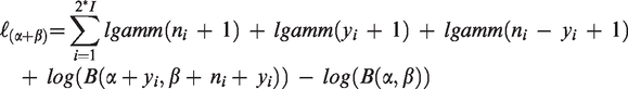
The log-likelihood written as a function of α and β is given by Skellam, ¹⁴ where we additionally use α = g(μ_i)[1− ρ]/ρ and β = [1 − g(μ_i)] [1− ρ]/ρ

$$\mathit{\ell }\mathrm{(}\mathrm{\alpha }\mathrm{+}\mathrm{\beta }\mathrm{)}\mathrm{=}\sum _{i=1}^{2^{\mathrm{*}}I}\mathit{lgamm}(n_i\mathrm{\hspace{0.17em}}+\mathrm{\hspace{0.17em}}1)\mathrm{\hspace{0.17em}}+\mathrm{\hspace{0.17em}}\mathit{lgamm}(y_i\mathrm{\hspace{0.17em}}+\mathrm{\hspace{0.17em}}1)\mathrm{\hspace{0.17em}}+\mathrm{\hspace{0.17em}}\mathit{lgamm}(n_i\mathrm{\hspace{0.17em}}-\mathrm{\hspace{0.17em}}{y}_i\mathrm{\hspace{0.17em}}+\mathrm{\hspace{0.17em}}1)\mathrm{\hspace{0.17em}}+\mathrm{\hspace{0.17em}}\mathit{log}\left(B\right(\alpha +y_i,\beta +\mathrm{\hspace{0.17em}}{n}_i+\mathrm{\hspace{0.17em}}{y}_i\left)\right)\mathrm{\hspace{0.17em}}-\mathrm{\hspace{0.17em}}\mathit{log}\left(B\left(\alpha ,\beta \right)\right)$$

where lgamm denotes the natural logarithm of the gamma function and B the beta function.

Common-beta model

Instead of assuming the two beta distributions in control and treatment groups to share the same correlation parameter ρ, we can assume that they share the same β, that is β = β_T = β_C. The three parameters to be estimated are then α_T, α_C, and β. Analogously to the “common-rho” model, we term this model the “common-beta” model. In the common-beta model the correlations (ρ_C, ρ_T) between individual observations in the control and the treatment groups would be different if α_T and α_C are different.

Unfortunately, this model can no longer be written as a regression model as above, but treatment effects must be estimated from α_T, α_C, and β by using μ_C = α_C/(α_C + β) and μ_T = α_T/(α_T + β). To be concrete, μ_T/μ_C describes the treatment effect as a relative risk, μ_T–μ_C as a risk difference, and μ_T(1–μ_C)/μ_C(1–μ_T) as an odds ratio. For the odds ratio, the log odds ratio can be conveniently estimated by α_T/α_C.

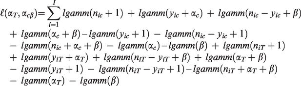
The log-likelihood of the model is

$$\mathit{\ell }\mathrm{(}{\mathrm{\alpha }}_T\mathrm{,}\mathrm{\hspace{0.17em}}\mathrm{\alpha }c\mathrm{\beta }\mathrm{)}\mathrm{=}\sum _{i=1}^I\mathit{lgamm}(n_{ic}+1)\mathrm{\hspace{0.17em}}+\mathrm{\hspace{0.17em}}\mathit{lgamm}(y_{ic}+{\alpha }_c)\mathrm{\hspace{0.17em}}+\mathrm{\hspace{0.17em}}\mathit{lgamm}(n_{ic}-y_{ic}+\beta )\mathrm{\hspace{0.17em}}+\mathrm{\hspace{0.17em}}\mathit{lgamm}({\alpha }_c+\beta )\mathrm{\hspace{0.17em}}–\mathrm{\hspace{0.17em}}\mathit{lgamm}(y_{ic}+1)\mathrm{\hspace{0.17em}}-\mathrm{\hspace{0.17em}}\mathit{lgamm}(n_{ic}-y_{ic}+1)\mathrm{\hspace{0.17em}}-\mathrm{\hspace{0.17em}}\mathit{lgamm}(n_{ic}+{\alpha }_c+\beta )\mathrm{\hspace{0.17em}}-\mathrm{\hspace{0.17em}}\mathit{lgamm}\left({\alpha }_c\right)\mathrm{\hspace{0.17em}}–\mathrm{\hspace{0.17em}}\mathit{lgamm}\left(\beta \right)\mathrm{\hspace{0.17em}}+\mathrm{\hspace{0.17em}}\mathit{lgamm}(n_{iT}+1)\mathrm{\hspace{0.17em}}+\mathrm{\hspace{0.17em}}\mathit{lgamm}(y_{iT}+{\alpha }_T)\mathrm{\hspace{0.17em}}+\mathrm{\hspace{0.17em}}\mathit{lgamm}(n_{iT}-y_{iT}+\beta )\mathrm{\hspace{0.17em}}+\mathrm{\hspace{0.17em}}\mathit{lgamm}({\alpha }_T+\beta )\mathrm{\hspace{0.17em}}-\mathrm{\hspace{0.17em}}\mathit{lgamm}(y_{iT}+1)\mathrm{\hspace{0.17em}}-\mathrm{\hspace{0.17em}}\mathit{lgamm}(n_{iT}-y_{iT}+1)\mathrm{\hspace{0.17em}}–\mathrm{\hspace{0.17em}}\mathit{lgamm}(n_{iT}+{\alpha }_T+\beta )\mathrm{\hspace{0.17em}}-\mathrm{\hspace{0.17em}}\mathit{lgamm}\left({\alpha }_T\right)\mathrm{\hspace{0.17em}}-\mathrm{\hspace{0.17em}}\mathit{lgamm}\left(\beta \right)$$

Connection between the common-beta beta-binomial model and the fixed-effect negative binomial regression model

In econometrics and the social sciences negative binomial regression models for panel count data models are often specified depending on the mean event rate per time unit.^12,15 If we parametrize the model with λ_failure = exp(c₀) and λ_success = exp(c₀ + c₁ + c_T), where c₀ is an intercept, c₁ is a binary indicator for success, and c_T is the interaction of c₁ and the treatment group, then Guimaraes could show that the common-beta model can be interpreted as a fixed-effect negative binomial regression (FE-NegBin) model for panel count data. ¹² To be concrete, if we set β = exp(c₀), α_T = exp(c₀ + c₁ + c_T), and α_C = exp(c₀ + c₁), then the likelihood of the common-beta model and that of a FE-NegBin coincide, premised the FE-NegBin is estimated by conditional maximum likelihood. ¹⁶

For the considered FE-NegBin the conditional log-likelihood function can be written as ¹⁷

$$\mathit{\ell }\mathrm{=}\sum _{i=1}^I\mathit{lgamm}\left({\lambda }_{i,\mathit{success}}+{\lambda }_{i,\mathit{failure}}\right)+\mathrm{\hspace{0.17em}}\mathit{lgamm}\left(y_{i,\mathit{success}}+{\lambda }_{i,\mathit{failure}}+1\right)+\mathrm{\hspace{0.17em}}\mathit{lgamm}\left({\lambda }_{i,\mathit{success}}+{\lambda }_{i,\mathit{failure}}+\mathrm{\hspace{0.17em}}{y}_{i,\mathit{success}}+{\lambda }_{i,\mathit{failure}}\right)+\mathrm{\hspace{0.17em}}\left(\mathit{lgamm}\left({\lambda }_{i,\mathit{success}}+\mathrm{\hspace{0.17em}}{y}_{i,\mathit{success}}\right)-\mathit{lgamm}\left({\lambda }_{i,\mathit{success}}\right)\right)-\mathrm{\hspace{0.17em}}\mathit{lgamm}\left({\lambda }_{i,\mathit{success}}+1\right)\mathrm{\hspace{0.17em}}+\mathrm{\hspace{0.17em}}\left(\mathit{lgamm}\left({\lambda }_{i,\mathit{failure}}+\mathrm{\hspace{0.17em}}{y}_{i,\mathit{failure}}\right)\right)\hspace{0.17em}+\mathrm{\hspace{0.17em}}\left(\mathit{lgamm}\left({\lambda }_{i,\mathit{failure}}+\mathrm{\hspace{0.17em}}{y}_{i,\mathit{failure}}\right)-\mathit{lgamm}\left({\lambda }_{i,\mathit{failure}}\right)\right)\hspace{0.17em}-\mathit{lgamm}\left({\lambda }_{i,\mathit{failure}}\right)-\mathrm{\hspace{0.17em}}\mathit{lgamm}\left({\lambda }_{i,\mathit{failure}}+1\right)\mathrm{\hspace{0.17em}}$$

where $y_{i,\mathit{success}}$ and $y_{i,\mathit{failure}}\mathrm{\hspace{0.17em}}$ denote the number of successes and failures, respectively.

Setting λ_failure = β and λ_success = α in this log-likelihood function makes the equivalence between the models obvious (compare log-likelihood function in section “Common-beta model”). ¹²

The estimate of the interaction term of c₁ and c_T from the FE-NegBin model equals the log odds ratio from the common-beta model α_T/α_C. The main treatment effect is not included in the model, and the term to be conditioned on here is the number of total counts in the group. Consequently, and similar to the BBST, the FE-NegBin ignores the fact that each control group is connected to a treatment group from the same study.

The equivalence between the models makes it possible to use panel count data estimation procedures as usually used in econometrics for estimating the common-beta BB/FE-NegBin model. Noteworthy, in panel count data the term fixed effects does not refer to the distribution of the variables but means that for each group an individual intercept is estimated.

When using the COUNTREG procedure in SAS® to fit the common-beta BB/FE-NegBin model, the dataset has to be structured so that each cell from a 2-by-2-table of a single study constitutes a single observation. To be exact, there should be two columns with binary indicators for treatment and success and a column (here: y) that gives the number of events in the respective cell. In addition, we need a column to indicate the study group. The structure of these dataset is illustrated in box 1. Box 1

Input dataset for two example studies to estimate a common-beta BB/FE-NegBin model in SAS^® PROC COUNTREG.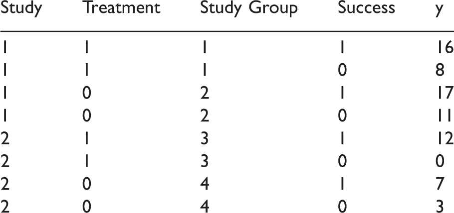

Study	Treatment	Study Group	Success	y
1	1	1	1	16
1	1	1	0	8
1	0	2	1	17
1	0	2	0	11
2	1	3	1	12
2	1	3	0	0
2	0	4	1	7
2	0	4	0	3

Box 2 contains an example SAS-code for re-structuring the dataset, and parameter estimation using PROC COUNTREG for the common-beta BB/FE-NegBin model for an example dataset (see below). Box 2

Example SAS-code for the FE-NegBin.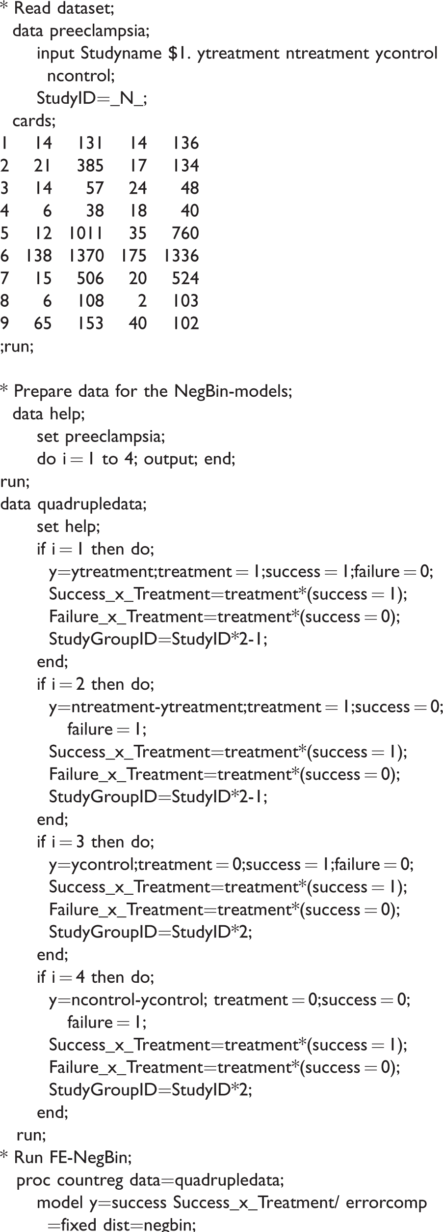

* Read dataset;

data preeclampsia;

input Studyname $1. ytreatment ntreatment ycontrol ncontrol;

StudyID=_N_;

cards;

1 14 131 14 136

2 21 385 17 134

3 14 57 24 48

4 6 38 18 40

5 12 1011 35 760

6 138 1370 175 1336

7 15 506 20 524

8 6 108 2 103

9 65 153 40 102

;run;

* Prepare data for the NegBin-models;

data help;

set preeclampsia;

do i = 1 to 4; output; end;

run;

data quadrupledata;

set help;

if i = 1 then do;

y=ytreatment;treatment = 1;success = 1;failure = 0;

Success_x_Treatment=treatment*(success = 1);

Failure_x_Treatment=treatment*(success = 0);

StudyGroupID=StudyID*2-1;

end;

if i = 2 then do;

y=ntreatment-ytreatment;treatment = 1;success = 0; failure = 1;

Success_x_Treatment=treatment*(success = 1);

Failure_x_Treatment=treatment*(success = 0);

StudyGroupID=StudyID*2-1;

end;

if i = 3 then do;

y=ycontrol;treatment = 0;success = 1;failure = 0;

Success_x_Treatment=treatment*(success = 1);

Failure_x_Treatment=treatment*(success = 0);

StudyGroupID=StudyID*2;

end;

if i = 4 then do;

y=ncontrol-ycontrol; treatment = 0;success = 0;failure = 1;

Success_x_Treatment=treatment*(success = 1);

Failure_x_Treatment=treatment*(success = 0);

StudyGroupID=StudyID*2;

end;

run;

* Run FE-NegBin;

proc countreg data=quadrupledata;

model y=success Success_x_Treatment/ errorcomp=fixed dist=negbin;

Random-effects negative binomial regression

Using the equivalence of the common-beta and the FE-NegBin model allows for some further insights from econometrics, the field where NegBin models are frequently used. For example, it is straightforward to generalize the FE-NegBin to a random effects negative binomial regression (RE-NegBin) model, namely a random effects negative binomial model for panel count data. Random effect in this model does not mean that there is an additional random effect included in the linear predictor, but that for the multiplicative dispersion parameter ξ for the expected number of counts (intercept) a random distribution is assumed. In the FE-NegBin model, this dispersion parameter ξ is also part of the model but can take on any value. Explicitly modelling ξ in the RE-NegBin model accounts for some additional unexplained overdispersion. Hausman et al. showed that if ξ/(1+ ξ) follows a beta distribution, then the resulting likelihood function has still closed form. ¹⁶ It should be noted that this beta distribution for the additional overdispersion parameter has nothing to do with the initial beta distributions from the parallel common-beta model.

Example

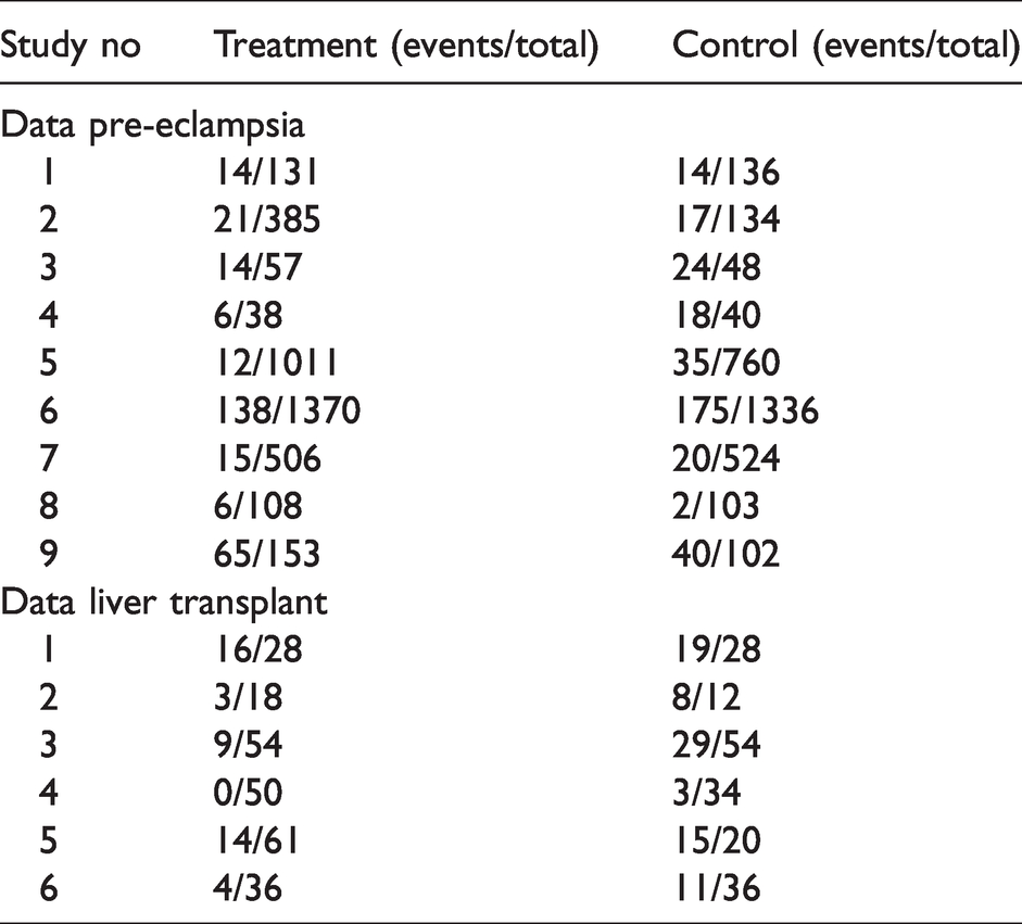
We illustrate the methods with two example datasets from actually performed meta-analysis. The first example is a meta-analysis of nine randomized controlled trials on diuretics for prevention of pre-eclampsia. ¹⁸ The second example is a meta-analysis of six observational studies assessing interleukin-2 receptor antagonists for paediatric liver transplant recipients to avoid acute rejection. ¹⁹ The example datasets are presented in Table 1.

Table 1.

Example datasets.

Study no	Treatment (events/total)	Control (events/total)
Data pre-eclampsia
1	14/131	14/136
2	21/385	17/134
3	14/57	24/48
4	6/38	18/40
5	12/1011	35/760
6	138/1370	175/1336
7	15/506	20/524
8	6/108	2/103
9	65/153	40/102
Data liver transplant
1	16/28	19/28
2	3/18	8/12
3	9/54	29/54
4	0/50	3/34
5	14/61	15/20
6	4/36	11/36

Simulation

To get initial insights in the performance of the models introduced here, we performed a small simulation study.

Design of simulation

We considered an “effect” scenario (H1) and a “no-effect” scenario (H0). All other parameters of the simulation were varied randomly and informed by actually performed meta-analyses to reflect realistic meta-analysis scenarios. The distribution of the number of studies was taken from a publication of Page et al., who analysed 119 non-Cochrane systematic reviews of randomized controlled trials and observational studies.^7,8 For all other design factors we used the review of Turner et al., which analysed 1,991 systematic reviews from the Cochrane Database of Systematic Reviews. ⁸ The factors varied and the distributions from which the respective values were drawn are shown in Table 2.

Table 2.

Description of the simulation.

Factor	Distribution	Properties of Distribution
Number of studies	Generated from a log-normal distribution with mean = 0.65 and SD = 1.2; truncation if >40	Median = 9, Q1 = 5, Q3 = 14
Sample size of a single study	Generated from a log-normal distribution with mean = 4.615 and SD = 1.1	Median = 103, Q1 = 50, Q3 = 204
Allocation of individual observations to control and treatment group	Bernoulli distribution with probability 0.5
Event probabilities in the control group	Generated from a beta distribution with α = 0.4230 and β = 1.433	Mean = 0.223, SD =  0.256 Median = 0.126
H1	Generated from an inverse‐variance random effects model (see column treatment effect and heterogeneity variance)
Treatment effect (odds ratio)	Generated from a log-normal distribution with mean = −0.59 and SD = 0.61	Mean = 0.671, SD =  0.188 Median = 0.691
Heterogeneity variance of treatment effect	Generated from a log-normal distribution with mean τ2 = −1.47, SD = 1.65, Skewness = −0.55	Median τ2 = 0.274, Q1 = 0.079, Q3 = 0.806

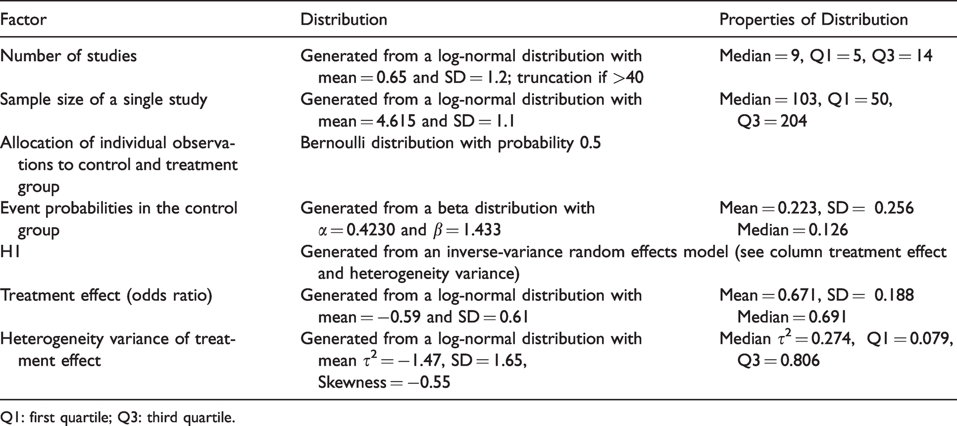
Q1: first quartile; Q3: third quartile.

We generated 10,000 meta-analyses for each scenario (H0 and H1).

Procedures for estimation

For estimation of the common-rho beta-binominal model we use SAS PROC NLMIXED and computed the starting values from raw proportions and their variances. For estimation of the common-beta common-beta/NegBin models we used SAS PROC COUNTREG.

Measures to assess performance of the methods

We used t-distributed confidence intervals (CIs) using I*2 $-$ 2 degrees of freedom for all methods because this showed best results regarding coverage probability in our previous simulation study. ⁶

We counted the number of converged runs to assess the numerical robustness. We estimated median bias with quartiles and the mean empirical coverage to the 95%-CIs to assess the performance of the models. ⁴ All results are reported on the log odds ratio scale.

Results

Example

The pooled results for all methods for the two examples are shown in Figures 1 and 2.

Figure 1.

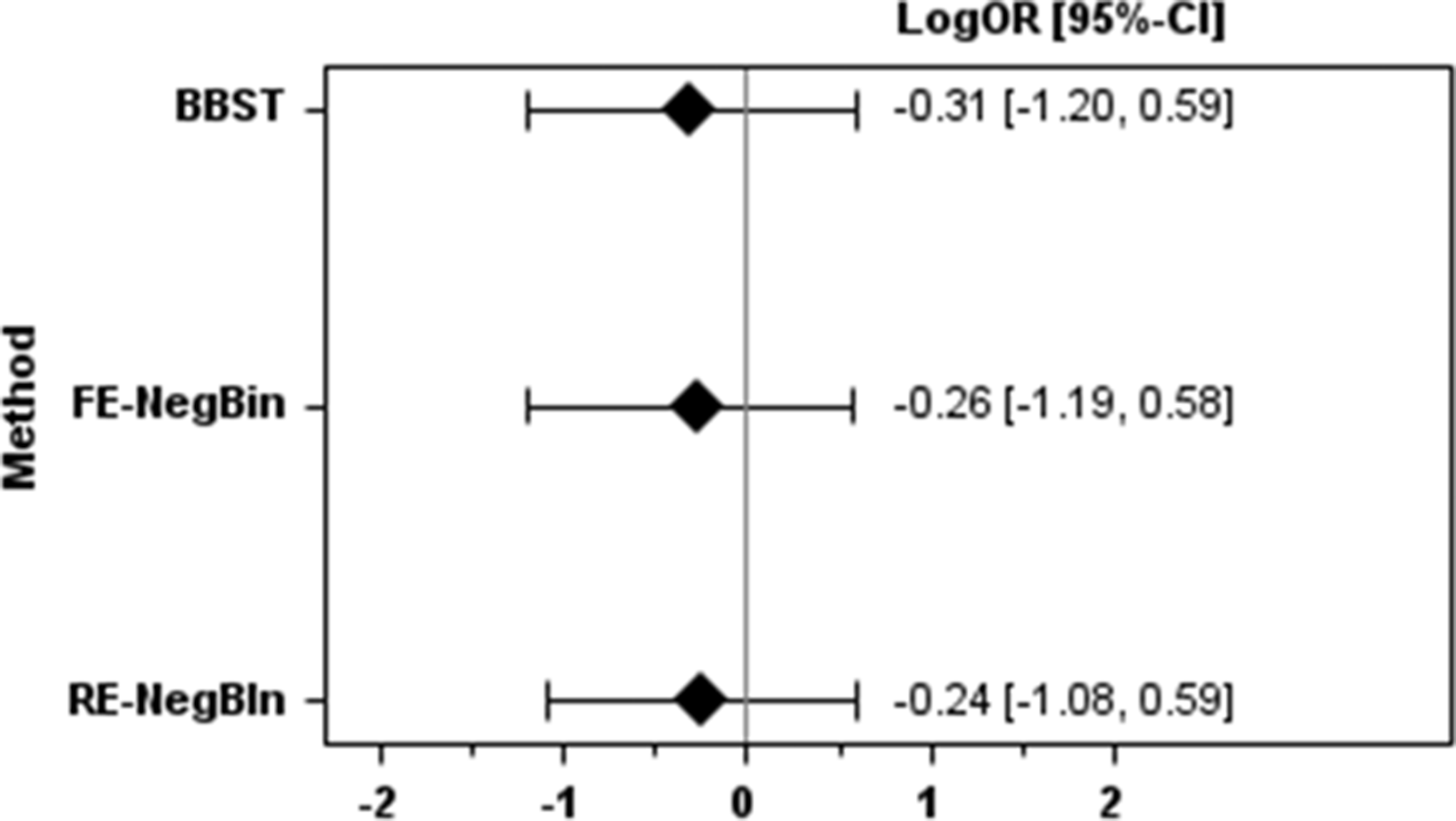
Results for the pre-eclampsia example.

Figure 2.

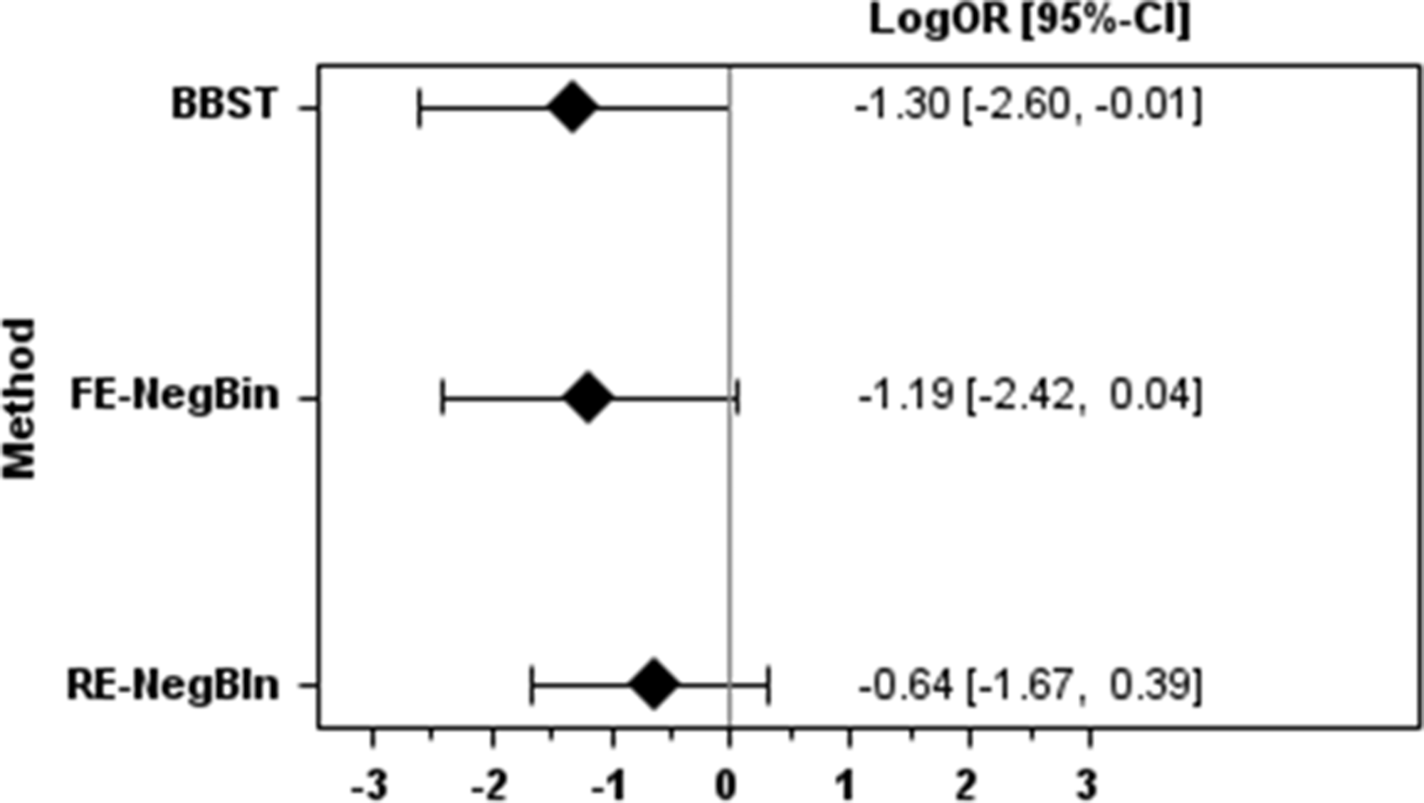
Results for the liver transplantation example.

Effect estimates were largest for the BBST, followed by FE-NegBin and RE-NegBin in both example datasets. The 95%CIs were narrowest for RE-NegBin for both examples. In the pre-eclampsia example all methods showed very similar results with regard to statistical significance. In the liver transplant example BBST reached statistical significance and FE-NegBin was nearly statistical significant. In contrast, the 95% CI of RE-NegBin clearly overlapped the no effect line.

Simulation

In Table 3 we present results for both simulation scenario. Figures 3 and 4 illustrate the performance in terms of bias and coverage for the “effect” scenario (H1).

Table 3.

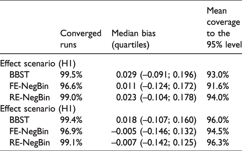
Results for performance measures.

	Converged runs	Median bias (quartiles)	Mean coverage to the 95% level
Effect scenario (H1)
BBST	99.5%	0.029 (–0.091; 0.196)	93.0%
FE-NegBin	96.6%	0.011 (–0.124; 0.172)	91.6%
RE-NegBin	99.0%	0.023 (–0.104; 0.178)	94.0%
Effect scenario (H1)
BBST	99.4%	0.018 (–0.107; 0.160)	96.0%
FE-NegBin	96.9%	–0.005 (–0.146; 0.132)	94.5%
RE-NegBin	99.1%	–0.007 (–0.142; 0.125)	96.3%

Figure 3.

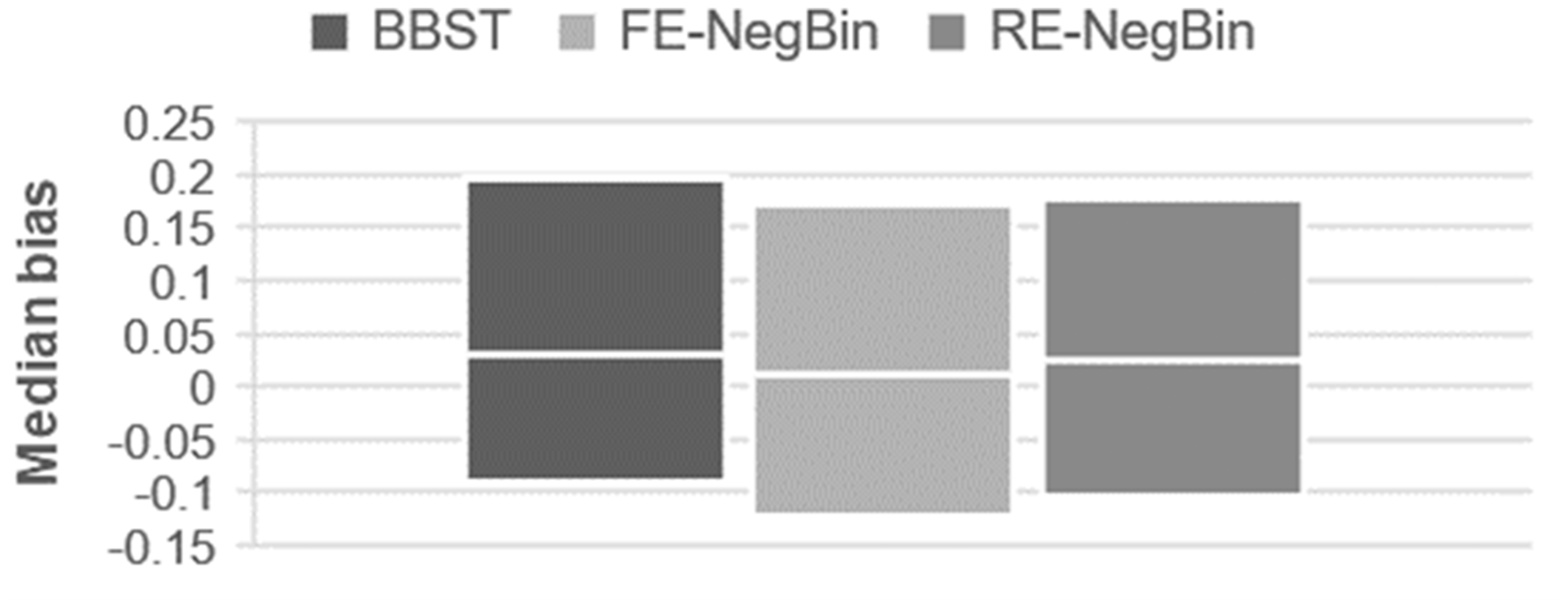
Median bias (with quartiles) in the “effect” scenario (H1).

Figure 4.

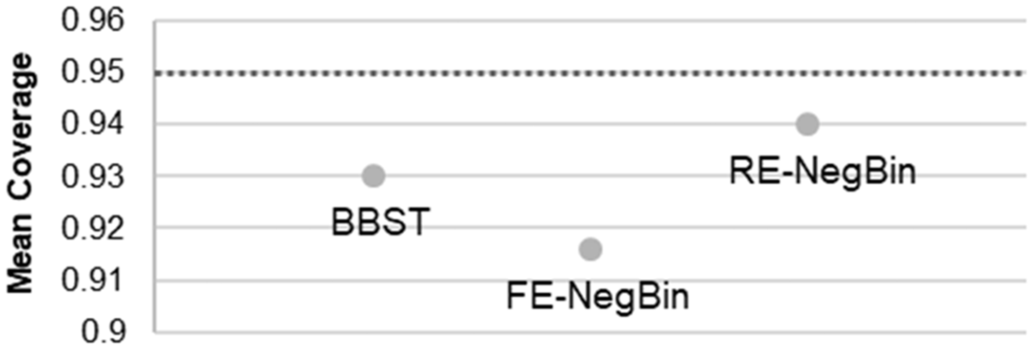
Mean empirical coverage to the 95% level in the “effect” scenario (H1).

With respect to numerical robustness, BBST and RE-NegBin converged in over 99% and FE-NegBin in about 97% of simulation runs.

Median bias was negligible for all methods in all scenarios. The upper quartile for bias suggested a marginally stronger bias for the BBST compared to the common-beta/NegBin models. Considering the lower quartile for bias the common-beta/NegBin models showed a slight tendency towards higher negative biases.

No method falls dramatically below the nominal coverage in any situation. Lowest empirical coverage overall was observed for the FE-NegBin in the “effect scenario” (0.92). The RE-NegBin performed best regarding empirical coverage, followed by BBST and FE-NegBin.

Discussion

In this paper we introduce the “common-beta” beta-binomial regression model for meta-analysis of binary outcomes and a new estimation approach by perceiving this common-beta model as a fixed-effect negative binomial (FE-NegBin) regression for panel count data. Generalizing the FE-NegBin to a random-effect negative binomial (RE-NegBin) allows for modelling an additional overdispersion parameter, while retaining a closed log-likelihood function. We illustrated the methods with two examples and a small-scale simulation study mirroring real-world non-Cochrane meta-analyses.

In our simulation study none of the methods had serious problems with parameter estimation, with the FE-NegBin model being a slight exception, probably because one fixed-effect must be estimated for each group.

Median bias was negligible for all methods. The upper quartile in the simulation and the examples suggest that BBST is most affected by positive bias (estimated treatment effects being larger than expected). This positive bias occurs in cases where the event probability is high and the heterogeneity between groups strongly differs. ²⁰

Regarding coverage probability, BBST and the RE-NegBin model outperformed the FE-NegBin model. The reason could be that in the BBST the variance is implicitly bounded by the common-rho assumption. Likewise, the multiplicative beta-distributed random parameter in the RE-NegBin bounds the dispersion of the model by the additional dispersion parameter (variance divided by mean) to be random. Both assumptions mitigate large variance differences between groups and thus the risk for an underestimation of the variance (in one group).

An advantage of the common-beta models introduced in this paper is that its application can be facilitated by using estimation routines for panel count data models (e.g. SAS PROC COUNTREG, Stata xtnbreg, R MASS-Package). This approach requires no extensive programing, only the dataset has to be rearranged. It is of course a limitation that using panel count data estimation methods only allows for odds ratios to be estimated. Noticeable, using a general-purpose procedure that allows coding the likelihood function by hand (e.g. SAS NLMIXED), it is also possible to implement other link functions and hence calculating risk differences or relative risks.

The presented panel count data approach for estimating the NegBin models opens the door for using any other panel count data model (e.g. poison regression) for meta-analysis. The equivalence between the common-beta and the FE-NegBin model is only given when the latter model is estimated by conditional maximum likelihood and when the conditioning is with respect to the single group. However, estimating FE-NegBin, and likewise RE-NegBin models is also possible when using other conditioning units. For example, using the respective study (and not the single study group) as the conditioning unit would estimate a model that avoids the separation of treatment and control group from the same study, an inherent feature of the “common-rho” as well as of the “common-beta” model. This approach would overcome “breaking of randomisation”. Exploring extensions of the BB/NegBin models for panel count data which respect randomisation appears promising for future work.

Our simulation study was only designed to get initial insights into the statistical properties of the newly introduced models for meta-analysis to assess their general potential. Thus, a limitation of our study is that we cannot draw any definitive conclusion regarding the comparative performance of different meta-analytic methods or regarding the performance in specific situations (e.g. rare events). Future studies are necessary that examine the statistical properties of the NegBin models considered here in comparison to other methods for meta-analysis such as the Hartung-Knapp method or generalized linear mixed models. As the BBST proved to perform well for meta-analysis of a small number of studies or rare events, it would be in particular interesting to assess whether the models perform similar well or even better in such situations with sparse data.

Conclusion

The introduced Common-Beta/NegBin models appear valuable extensions to the family of BB models and potential candidates to be included in the meta-analysis toolbox. The feature that they can be quite easily implemented using standard statistical software make them especially appealing. However, before use in practice, future studies are necessary that assess their statistical properties in more depth and in comparison to other meta-analyses methods.