
Abstract
A technique is proposed for a more structured approach to modelling over- and under-dispersed counts: variance factorized loglinear (VFL) models are a parameterization of an (enlarged) distribution whereby the overdispersed variance is expressed as a product of the nominal variance and a remainder term involving a highly interpretable loglinear effect with a potentially different set of covariates. This facilitates mean–variance analysis by allowing the variance to be modelled more separately from the mean, especially for generalized linear models (GLMs). Consequently, VFL parameterized models offer substantial advantages over existing methods for investigating overdispersion, such as a unifying framework and greater interpretability. Examples given here of enlarged distributions that supply the equidispersion as a special case include the extended beta-binomial (with a newly proposed ‘clog’ link and special offset) and negative binomial (NB) and generalized Poisson (GP–1 and GP–2 variants). VFL parameterized models are constructed as a vector generalized linear model (VGLM) with a judicious combination of constraint matrices, offsets and link functions. Underdispersed data can be handled by expanding the response by a multiplier and offset adjustment. Useful for disentangling the mean–variance relationship in GLMs, VFL parameterized models are implemented within the very broad framework of the vector generalized additive model (VGAM) R package available from comprehensive r archive network (CRAN). The technique is generally applicable to mean-parameterized distributions.
Keywords
Introduction
Overdispersed counts commonly encountered in applied statistics are analyzed by a variety of techniques ranging from rigourous to ad hoc. For this, previous work such as Nelder and Lee (1991), Hinde and Démetrio (1998) and Carroll (2003) have sought and emphasized structure and the purpose of this article is to propose a technique for constructing or defining/identifying a subclass of models that aids such an analysis in a more systematic manner. In particular, the aim here is to enable and/or disentangle mean–variance modelling so that each part sheds separate insight into the trend and variability. We call this mean–variance analysis (MVA) where the purpose is to separately focus on the mean and variance of an (enlarged) model having two parameters. Although the binomial and Poisson cases are the main examples, the concepts carry over well beyond the generalized linear model (GLM; Nelder and Wedderburn, 1972) and to underdispersed data too (Section 4). Two main motivations for variance factorized loglinear (VFL) parameterized models are given in Section 2. The methological contribution of this article is a proposal of a technique for parameterizing a distribution so that MVA is facilitated. Although applied in this article to four distributions, the technique is general and can be applied beyond the examples here.
Write the data as (

where Ve(μ;
We now summarize the class of vector generalized linear models (VGLMs; Yee, 2015) which conveniently fit VFL parameterized models because they have the necessary framework and infrastructure. The framework is very large so that it easily accommodates all the variants of Table 1. The log-likelihood to be maximized is

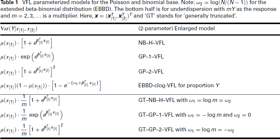
VFL parameterized models for the Poisson and binomial base. Note: ω2 = log(N/(N − 1)) for the extended beta-binomial distribution (EBBD). The bottom half is for underdispersion with mY as the response and m = 2, 3, … is a multiplier. Here,
.and ‘GT’ stands for ‘generally truncated’.
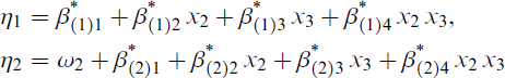
for j = 1, …, M and some suitable parameter link function gj because gj operates on a parameter rather than to a mean only. The β(
j
)
k
in (1.2) reflect the two-dimensional structure of the regression coefficients: Across the jth linear predictor and across the kth covariate, which is reflected by 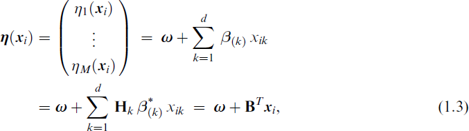
for known constraint matrices 
is a possibly reduced set of regression coefficients to be estimated. The
From the vast number of methods proposed for unequidispersed count regression it is beneficial comparing several to highlight issues and differences with this work. In general, a MVA requires a mean-parameterization and the variance is usually the other parameter or is somewhat related to (1.1).
Fisher scoring used for VGLM estimation essentially only requires the expected information. Work such as Cifuentes-Amado and Cepeda-Cuervo (2024) is partly based on this algorithm, however it is far more complex, Bayesian and no software is available. Somewhat similar is the compound Poisson-normal model of Hinde (1982) estimated by iteratively reweighted least squares, numerical integration and the expectation–maximization (EM) algorithm. However, while a generalized linear interactive modelling (GLIM) macro is given, there is no R implementation and the author states its results are expected to be very similar to negative binomial (NB) regression.
One approach is based on mixtures such as the Poisson–Tweedie (e.g., Petterle et al., 2019; Abid et al., 2021) which have a variance such as μ + ϕμp and μ + μ2 + ϕμp. These have several disadvantages such as the dispersion ϕ and power p parameters can only be modelled as intercept-only. In terms of interpretation, neither of these models is a suitable vehicle for MVA. Furthermore, neither of these models is as simple as (3.1), (3.2) or (3.3) below.
In recent years Conway–Maxwell–Poisson regression has received considerable attention (e.g., Shmueli et al., 2005; Sellers, 2023), however there are numerical challenges such as computing its normalizing constant and expected information. Unfortunately the mean-parameterized variant (Huang, 2017) also suffers from these drawbacks. Another distribution whose normalizing constant is difficult to compute is del Castillo and Pérez-Casany (2005) even though the model may be reparameterized by the mean and variance ‘under certain assumptions’. Yet another approach is to use quasi-likelihood rather than maximum likelihood estimation, (e.g., Engel and Brake, 1993, for proportions), however such methods do not allow the dispersion parameter ϕ to incorporate covariates.
To summarize, the above work and most others tend to be piecemeal in nature and if software has been written, specialized algorithms are required and it is limited to that specific model only. Also, often these works do not promote MVA because they lack the interpretability needed (e.g., (1.1)) and any overdispersion parameter cannot realistically incorporate covariates, as well has being computationally complex.
Motivating considerations
There are many instances where understanding the structure of variability is just as central as understanding the mean structure (Carroll, 2003). Under such conditions, if the variance structure is treated as a nuisance instead of being a central part of the modelling effort, it will lead to inefficient estimation of means and to misleading conclusions. One such instance where the mean–variance relationship has a central property is the case of multivariate abundances (Warton and Hui, 2017), where potentially serious artifacts can be introduced to analyses if this is not accounted for.
Under this setting, VFL parameterized models are spurred by two main motivations. Before describing these, it is emphasized that the technique is amenable to any mean-parameterized distribution and not only for counts. The methodology seeks to untwine the mean and the variance using two simple features available in the VGLM infrastructure (constraint matrices and offsets).
The first motivation is that (1.1) has several compelling advantages. Foremost, it allows variation in the response to be studied more separately from the signal. For example, in quantitative finance, the volatility may be of equal interest as the trend so that the ability to unravel the signal–noise relationship is crucial. Electrocardiography is another example where variability may be more important than the trend. Since Ve is a simple function of the mean for GLMs, another advantage is that the VFL approach teases out the mean–variance relationship so that interpretation is greatly facilitated. A different set of covariates may be used to model the mean and remainder terms, hence overdispersion can be modelled separately and conditional on μ. This follows the rationale of quasi-likelihood modelling, for example, having

where a moment estimator of the dispersion parameter, They are modular and belong to a large framework. Because they arise from a choice of They are very interpretable because loglinear models exhibit multiplicative effects. In contrast, under- and overdispersion is less interpretable for Conway–Maxwell–Poisson regression (for example) even when mean-parameterized because the variance is a complicated function of the parameters. In addition to VGLMs, the framework of Yee (2015) provides other useful classes such as the VGAM of Section 5.3 for additive modelling, to provide a data-driven approach by smoothing.
The second motivation is computational. For ordinary two-parameter models the constraint matrices The framework means that each VFL parameterized model can be implemented in R by a single ‘family’ function; for example, Ease of implementation: It is almost trivial constructing the appropriate Fisher scoring is well-established and mainstream (Osborne, 1992). Convergence is rapid and standard errors are automatically produced from scoring.
It is noted that for MVA a direct mean–variance parameterization is often problematic, for instance, estimation for the NB distribution parameterized by its mean and variance, NB(μ, σ2), having probability mass function

involves a difficult constrained optimization because η1 < η2 when the log link is applied to both parameters. VFL parameterized models are a pragmatic compromise.
We look separately at overdispersion relative to the Poisson and binomial distributions.
Poisson and the NB, GP-1 and GP-2
Consider Y ∼ NB(μ, κ) as the ‘enlarged’ distribution with η1 = log μ and η2 = log κ as μ and κ are positive. Then based on Var(Y) = μ(1 + μ/κ), a VFL parameterized model is obtained by choosing 
with the Poisson limit μ/κ → 0+ defining Y* ∼ Pois(μ). Thus it is possible to distance the mean from the variance with respect to
Practically, one procedure is to make a copy of all the covariates used for μ and fitting a model with
We now apply same argument to two variants of the generalized Poisson distribution.

which is very interpretable.

so that it is similar to the NB–H–VFL (3.1) but the standard deviation is modelled instead of the variance.
Collectively, (3.1), (3.2) and (3.3) enable overdispersion for counts to be modelled more separately from the mean so that one can perform variance modelling, given μ. Table 1 and Appendix B are a summary. All three equations have compelling advantages over the quasi-Poisson variance (2.1): They allow ϕ to be effectively modelled with
Compared to the classical beta-binomial, the EBBD (Prentice, 1986) has the advantage of accommodating a small amount of underdispersion. This is very useful when units within a cluster are independent because of sampling variation. The EBBD for a proportion y has probability mass function
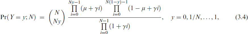
where N > 1, μ = E(y) ∈ (0, 1), γ = ρ/(1 − ρ) and 
and Var(NY) = Nμ(1 − μ)[1 + (N − 1)ρ]. The classical beta-binomial replaces the lower bound of (3.5) by 0, therefore the EBB test for independence does not involve hypothesis testing at the parameter space boundary so that Tarone’s Z statistic (Tarone, 1979) is unnecessary. This is the second favourable property described very shortly. It is now shown that

is a VFL parameterized model with two favourable properties. Note that the link proposed here for η2 is an incomplete complementary log–log link function, which is named the complementary log (‘clog’) link instead of the usual ‘cloglog’.

where ω2 = log(N/(N − 1)). □
The first significant result is that
The second favourable property of (3.6) is that if η2 is intercept-only then testing H0 : ρ = 0 is equivalent to testing H0 : β(2)1 = 0, for example, using the ordinary Wald statistic produced by
Most count distributions suitable for use as the enlarged distribution cannot handle underdispersion; for example, NB, GP–1, GP–2 for the Poisson.A natural question is: How can VFL parameterized models handle underdispersed responses? A practical solution is offered in this section. Because the left-hand side of (1.1) is of the enlarged distribution, the loglinear term R(μ;
We want

for some Y-transformed Y* not exhibiting underdispersion. A suitable transformation is Y* = mY for some integer multiplier m > 1. Using the Poisson as the ‘baseline’ count distribution then (4.1) becomes m Var(Y)/μ = R(μ, θ2) ≥ 1. Applying this to the NB distribution for example, one obtains the NB–H–VFL model having

For estimation it is recommended that the smallest m achieving unequivocal overdispersion be used; for example, we want a finite
Strictly, a more accurate approximation is mY ∼ GT–NB (Yee and Ma, 2024) with truncation set

where ‘GT’ is an abbreviation for ‘generally truncated’. The simulation study below shows that without general truncation, the estimates are not consistent. Although the coefficients for μ(
It is noted that an alternative to (4.2) is to omit the offset for η2 so that

While this special case is just as interpretable, we believe the bottom half of Table 1 is preferable because they share a common format. It is also noted that relatively few distributions are capable of modelling underdispersion (e.g., Sellers and Morris, 2017) and therefore can theoretically serve as the base distribution for the generally truncated expansion (GTE) method behind (4.3).
A final note here is that recently Puig et al. (2024) described mechanisms leading to under- and over-dispersion and commented that while both are common, underdispersion is less frequent. Possibly one might consider the multiplier m as a way to compensate for binomial thinning which is one mechanism for underdispersion. For the mean-parameterized distributions considered in this article it is informative knowing the conditions characterizing all two-parameter count distributions that are partially or fully closed under addition so that the maximum likelihood estimator of the population mean is the sample mean; for more details see Puig (2003) and Puig and Valero (2006).
In the following, we chose
Length of hospital stay in cardiovascular patients
We consider 3 589 cardiovascular patients’ Y = length of stay (LOS; days) in hospitals in Arizona, USA, around 1991. Being integer-valued, it is reasonable treating the response as having a count distribution. The data, available as
An ordinary NB–H regression would have the form
NB–VFL regression fitted to Arizona cardiovascular patients length of hospital stay: Final model. The suffix ‘.cp’ means a copy; for example, x1.cp = 1.
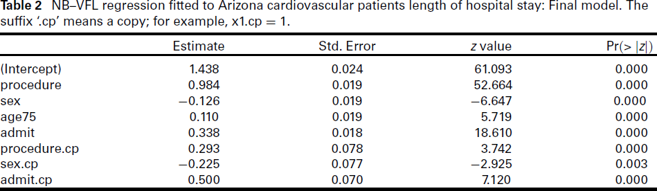
NB–VFL regression fitted to Arizona cardiovascular patients length of hospital stay: Final model. The suffix ‘.cp’ means a copy; for example, x1.cp = 1.
We fitted a VFL NB–H followed by backward elimination, which dropped In terms of the mean LOS, percutaneous transluminal coronary angioplasty (PTCA) have a shorter duration compared to coronary artery bypass graft (CABG), males have shorter stays, emergencies results in longer stays than elective treatment and increasing age is associated with longer stays. For example, the model predicts those aged over 75 have a mean LOS of e0.11046 − 1 ≈ 11.7% higher than those younger, cf. 12.0% empirically. The Because the intercept is omitted from
On the whole, a higher mean is associated with a higher variance for each variable, which has clinical implications.
Sleep duration data was obtained from a large New Zealand cross-sectional study called
Initially we fitted the NB–H–VFL (4.2) and GT–NB–H–VFL (4.3) with An increasing age is associated with a decreasing mean sleep duration and increasing overdispersion. This feature holds because if xk appears in both η1 and η2 then a sufficient condition for an increase in overdispersion due to incrementing Two more examples of the previous point are Maori and Polynesians compared to Europeans. The effect is most strongly associated with Polynesians. There are several possible explanations why this might be, such as the group being more heterogeneous in life style and work life compared to the other ethnicities (Tautolo et al., 2020; Fangupo et al., 2022). Divorcees and widows appear to experience lower mean sleep duration relative to singles, because the estimates −0.038 and −0.037 are negative and highly significant. There is weak evidence (p ≈ 0.045) of overdispersion among divorcees. The model suggests a very small mean difference between males and females, which are confirmed by predicted and empirical results showing that males sleep about 100(1 − e−0.022)/7 ≈ 0.3% to 0.6% less on average compared to females.
GT–NB–VFL regression fitted to underdispersed New Zealand health study sleep duration: Final model. The suffix ‘.cp’ means a copy; for example, x1.cp = 1.
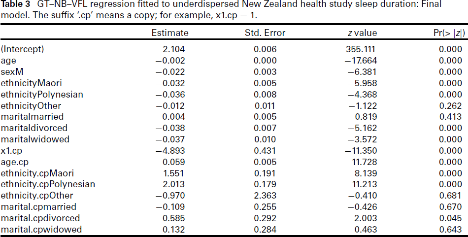
GT–NB–VFL regression fitted to underdispersed New Zealand health study sleep duration: Final model. The suffix ‘.cp’ means a copy; for example, x1.cp = 1.
Marginal statistics in the supplementary material confirm these results, as well as additional GP–1–VFL and GP–2–VFL analyses showing similar results to the NB–H–VFL, which is of no surprise due to the close similarity of the GP and NB distributions (Joe and Zhu, 2005).
We fit an EBBD to the number of chromosome aberrations in survivors across two atomic bombs. The number of analyzed cells was Ni = 100 for each individual and the covariates were x2 = dosage1
/
3 (rads) and x3 = site (640 survivors in Hiroshima as the baseline category and 399 in Nagasaki). The data
Extended beta-binomial regression for chromosomal aberrations due to radiation: Final model. This VFL parameterized model has variance (3.7). In the notation of (1.4), the regression coefficients are
respectively. The suffix ‘.cp’ means a copy; for example x1.cp = 1.
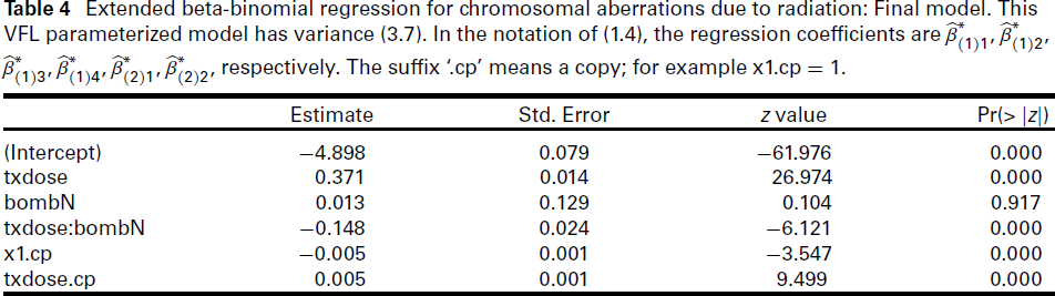
Extended beta-binomial regression for chromosomal aberrations due to radiation: Final model. This VFL parameterized model has variance (3.7). In the notation of (1.4), the regression coefficients are
respectively. The suffix ‘.cp’ means a copy; for example x1.cp = 1.
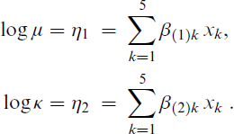
Fitting a VGAM, (Yee and Wild, 1996), it was found that x2 = dose1
/
3 gave a large improvement in linearity to both ηj. Denoting the bomb site by the indicator variable x3 with Hiroshima as the baseline, a joint model (3.6) was fitted having
with ω2 = log(100/99). Upon convergence, backward elimination removed the estimates of
At a zero radiation dose in Hiroshima,
The supplementary material reports on a simulation study conducted to compare the performance of the NB–H–VFL and GT–NB–H–VFL parameterized models relative to the quasi-Poisson for over- and under-dispersed data. The details are sketched here and results summarized. The overdispersed NB–H case had log μ = η1 = 1 + 2x2,

for n = 100, 500, 1 000 and x2 and x3 ∼ U(0, 1) independently. Six covariates were entered and backward elimination based on akaike information criterion was used for variable selection. The correct model was found with proportions 0.42, 0.66, 0.69 for these n values, respectively, showing that large sample may be needed for recovering the true model. The root mean square error showed a strongly decreasing sequence in n for μ and a more slowly decreasing sequence for κ. Wald confidence intervals were shown to work well in terms of their 95% coverage rates. The quasi-Poisson model was confirmed to have moment estimator ϕ consistent with the overall mean

Some conclusions are: (a) The NB–H–VFL model performs estimation well as a function of n although a larger n is required for precise estimation of the coefficients in R(μ;
The underdispersed case fitted data generated from GT–NB–VFL(mμ1, mκ1) with multiplier m = 4, η* = −1.5 + x3 and

with ω1 = ω2 = log m. For this, the NB–H–VFL produced biased estimates for
Understanding the structure of variation in counts continues to be an important problem (Carroll, 2003). VFL parameterized models address this need by providing additional insights into the variance structure conditional on the mean. The quest for methods to model the mean and variance separately has led to proposals such as some of those mentioned in Section 1.2, quasi-likelihood (Wedderburn, 1974), joint GLMs (Nelder and Lee, 1991), extended Poisson process models (EPPMs; e.g., Faddy, 1997; Faddy and Smith, 2008, 2011; Smith and Faddy, 2016, 2019) and double exponential families (Efron, 1986). All these are not without their shortcomings; for example, the latter may use a normalizing constant that can only be approximated and as mentioned in Section 3.1, quasi-likelihood cannot handle dispersion parameters with covariates, nor are ordinary standard errors available for confidence intervals without some adjustment. Likewise, EPPMs have complicated mean and variance expressions and lack the simplicity of (1.1)—covariate dependence in the variance is also complex.
For practitioners primarily interested in the mean structure, VFL parameterized models still offer benefit because how well the dispersion parameter is modelled affects the quality of the mean estimate. Taking the NB–H fitted by
Footnotes
Appendix
Acknowledgements
The author is grateful to the referees and editors whose comments greatly improved earlier versions of the manuscript.
Declaration of Conflicting Interests
The authors declared no potential conflicts of interest with respect to the research, authorship and/or publication of this article.
Funding
The authors received no financial support for the research, authorship and/or publication of this article.
Supplementary material
References
Supplementary Material
Please find the following supplemental material available below.
For Open Access articles published under a Creative Commons License, all supplemental material carries the same license as the article it is associated with.
For non-Open Access articles published, all supplemental material carries a non-exclusive license, and permission requests for re-use of supplemental material or any part of supplemental material shall be sent directly to the copyright owner as specified in the copyright notice associated with the article.