Sage Journals: Discover world-class research

Abstract

Background. Difference-in-Difference makes a critical assumption that the changes in the outcomes, over the post-treatment period, are similar between the treated and control groups—the parallel trends assumption. Evaluation of this assumption is often done either by graphical examination or by statistical tests in the pre-treatment period. They result in a binary conclusion about the validity of the assumption. Purpose. This paper proposes a sensitivity analysis that quantifies the departure from parallel trends necessary to meaningfully change the estimated treatment effect. Results. Sensitivity analyses have an advantage over traditional parallel trends tests: they use all available data and thereby work even if only one pre-period is available, and they quantify the strength of unobserved confounder(s) required to change the conclusions of a study. Conclusions. We apply the sensitivity analysis metrics developed by Cinelli and Hazlett (2020) and illustrate them on two studies.

Keywords

Difference-in-difference parallel trends sensitivity analysis

Introduction

Controlling for all confounders is a primary challenge of estimating a causal effect in an observational study. Confounders pose a threat to the unbiased estimation of a causal effect because of their relationship with both treatment assignment and the outcome, which could lead to a spurious result. Such a result arises when the effect of an unobserved confounder acting on the treatment and the outcome is confused with the effect of treatment. For example, the decision of a state to expand Medicaid under the Affordable Care Act (ACA) in 2014 was likely driven by multiple variables such as economic conditions, political landscape, and state finances, which may also influence outcomes of interest such as state spending on Medicaid. Longitudinal data is often used to estimate the causal effects of policies and programs. Causal analysis of longitudinal data is subject to confounding from both time-invariant and time-varying confounders. To estimate a causal effect, one needs to control for confounding from both sources.

Difference-in-difference is commonly applied to estimate causal effects in longitudinal data, especially in health policy.¹ To identify a causal effect, difference-in-difference removes time-invariant confounding by differencing (estimating a difference between) pre- and post-treatment periods. A second difference is then taken between the treated difference and the control difference to remove time-varying confounding. The second difference, however, assumes that the control unit(s) experience all the same time-varying confounders as the treated unit(s).

The assumption that the control unit experiences the same magnitude and type of time-varying confounding as the treated unit is known as the parallel trends assumption. If the underlying trends between treatment and control units are not in fact parallel, then the impact of unobserved confounders would be erroneously attributed to the treatment effect resulting in bias of unknown magnitude and often unknown direction. Therefore, the parallel trends assumption is far from innocuous.

Hypothesis tests are frequently used to assess the validity of the parallel trends assumption. A key concern with the indirect tests is that they only examine whether the parallel trends assumption is valid in the pre-period. For example, it is common for researchers to interact a time-invariant treatment indicator with time dummies and evaluate the significance of the coefficient for periods prior to treatment. This approach is problematic because there is no guarantee that if parallel trends hold in the period just prior to treatment, it will also hold in the treatment period.

An additional limitation of using hypothesis tests to evaluate parallel trends is a hypothesis test cannot confirm the null hypothesis (the trends in the two groups are parallel) nor can it quantify the departure from the null when the null is rejected. Hypothesis tests can only reject the null hypothesis based on the available evidence and cannot accept the null hypothesis is true. Furthermore, hypothesis tests do not evaluate the degree to which the null hypothesis is violated. In the case of parallel trends, it may be such that the assumption is violated enough to be statistically significant—such as in large sample sizes—but not enough to meaningfully change the estimated treatment effect.

An alternative approach is to use sensitivity analysis to find the smallest deviation from parallel trends that would undermine the conclusions of the original analysis, which assumes the parallel trends assumption is true. There are numerous prominent examples of this general idea. See, for example, Cornfield et al. (1959) about the link of smoking and lung cancer, and the development of this theme, leading to P. Rosenbaum’s papers (1987, 1988) and monographs about sensitivity to hidden bias in observational studies.^2–4

A suite of sensitivity analysis metrics developed by Cinelli and Hazlett (2020) focuses on the implementation of formal sensitivity analyses—to be discussed in the next section—for standard linear regression.⁵ Traditionally, discussions focus on whether unobserved confounders exist and place emphasis on the researcher controlling for all confounders. In much empirical work, however, it is challenging to control for all confounders, and impossible in the presence of unobserved confounding. The metrics developed by Cinelli and Hazlett enhance the discussion of unobserved confounders by quantifying how strong unobserved confounders need to be to change the conclusions—point estimate or statistical significance—drawn from a study. In this sense, the sensitivity analysis metrics are a way to judge the bias of an estimate in scenarios where it is difficult or impossible to control for all unobserved confounders.

This paper extends established sensitivity metrics to difference-in-difference analysis, with a focus on assessing the validity of the parallel trends assumption. In the context of difference-in-difference, the sensitivity metrics assess the validity of the results to a range of departures from the strict parallel-trends assumption. The metrics have three valuable characteristics. First, they utilize the post-period (post-treatment) data as well as pre-period (pre-treatment) data, which means the metrics can be estimated when there is only one pre-period. Second, they quantify how much stronger the unobserved time-varying confounder(s) need to be, relative to an observed time-varying confounder, to materially change the conclusions of the study. Third, the metrics invite discussion, based on expert content knowledge, of the plausibility that a time-varying unobserved confounder(s) of a given strength, exists.

This paper begins by reviewing the Omitted Variable Bias (OVB) framework, shows how Cinelli and Hazlett reparameterize it to develop their sensitivity analysis metrics, and extends those metrics to difference-in-difference. Then, two applied examples of the sensitivity metrics are discussed. Finally, the paper discusses this method and relates it to other methods for OVB such as VanderWeele’s E-value⁶ and Oster’s bounding approach.⁷

Background

The threat to causal inference in difference-in-difference models that is posed by potentially non-parallel trends between the treatment and control groups is an omitted variables-bias problem. The risk is that there is some unobserved—and therefore uncontrollable—factor that is causally linked to both the treatment status and the outcome. For example, when using difference-in-difference to test the effect of a policy change such as Medicaid expansion under the Affordable Care Act on an outcome such as the number of people uninsured, the Medicaid expansion could be determined in part by a state’s political climate, and this climate could also be causally related to intermediate variables such as how difficult it is to enroll in Medicaid even when eligible, and therefore to the outcome of interest such as the number of people insured. To the extent that this political climate is changing over time in ways that are unobserved, it poses a threat to causal inference in difference-in-difference.

The method here contextualizes this inferential threat rather than trying to control it. We place bounds on how strongly correlated such unobservable factors must be with both the treatment status and the outcome to eliminate any possible causal interpretation from the difference-in-difference estimates. There are three approaches discussed here.

1. The Robustness Value posits that the correlation of the unobserved time-varying factor with the treatment status and the outcome is the same and asks how large this correlation must be to eliminate the causal interpretation of the difference-in-difference estimates.

2. The Extreme Scenario Value posits that the unobserved factor is fully associated with the outcome and asks how strongly it must be correlated with the treatment to eliminate the causal interpretation of the difference-in-difference estimates.

3. The Relative Confounding Strength Value starts by noting the correlation of observed confounders with the treatment and outcome and asks what multiple of this correlation must be present for an unobserved confounder to eliminate the causal interpretation of the difference-indifference estimates.

The interpretation of these measures requires expert content knowledge. They are not statistical tests but guides to causal plausibility.

Each of these approaches is formally presented in what follows.

The classical omitted variable bias framework begins with the following equation for the true data generating process

Y = \hat{τ} D + \hat{β} X + \hat{γ} Z + {\hat{ϵ}}_{f u l l}

(1)where Y is the observed outcome, D is an observed treatment indicator,

\hat{τ}

is the estimated Average Treatment effect on the Treated (ATT), X is an observed covariate with an estimated coefficient

\hat{β}

, Z is an unobserved covariate with an estimated coefficient

\hat{γ}

, and

{\hat{ϵ}}_{f u l l}

is the random noise. Since Z is not observed, the restricted model is fitted

Y = {\hat{τ}}_{r e s} D + {\hat{β}}_{r e s} X + {\hat{ϵ}}_{r e s}

(2)where

{\hat{τ}}_{r e s}, {\hat{β}}_{r e s}

, and

{\hat{ϵ}}_{r e s}

are the coefficient estimates when Z is not included in the regression. The question is, how does

{\hat{τ}}_{r e s}

compare to

\hat{τ} ?

The classical OVB solution answers this as

{\hat{τ}}_{r e s} = \hat{τ} + \hat{γ} \hat{δ}

(3)where

\hat{γ}

—as in equation (1)—describes how the unobserved confounder Z impacts the outcome—the covariance of Z with D, and

\hat{δ}

describes how imbalanced the treatment and control groups are on Z conditional on X. When

\hat{γ}

is equal to zero—Z has no relationship with the outcome—then

{\hat{τ}}_{r e s} = \hat{τ}

; and the same holds when

\hat{δ}

is zero. However, when

\hat{γ}

and

\hat{δ}

are non-zero, then

{\hat{τ}}_{r e s}

is a biased estimator of

\hat{τ}

. Therefore, omitted variable bias is attributable to the product of the imbalance of unobserved factors across treatment and control groups, and the impact of those unobserved factors on the outcome.

In econometrics, the OVB framework is used to evaluate the bias that may be induced by unobserved confounders by using the hypothesized directionality of the partial correlation of the confounder with the outcome (impact or $\hat{γ}$ ) as well as with treatment (imbalance or $\hat{δ}$ ). The classical OVB framework, however, has several limitations that reduce its functionality to simple scenarios with a single binary confounder. The main shortcoming is the difficulty of generalizing classical OVB to multiple confounders. For example, if there are confounders Z1, Z2, and Z3, combining their partial correlations with the outcome and with treatment becomes difficult because of the many ways in which these confounders may combine. Motivated by these limitations, Cinelli and Hazlett reformulate the classical omitted-variables framework using an R² parameterization to obtain

| \hat{b i a s} | = s e ({\hat{τ}}_{r e s}) \sqrt{\frac{R_{Y \sim Z | D, X}^{2} \cdot R_{D \sim Z | X}^{2}}{1 - R_{D \sim Z | X}^{2}} (d f)}

(4)where

R_{Y \sim Z | D}^{2}

is the partial R² of Y with respect to Z after controlling for D (or the variance of Y that would be explained by Z after accounting for D) as well as for all of the observed confounders, X .

R_{D \sim Z | X}^{2}

is the partial R² of D attributable to Z when controlling for X .

s e ({\hat{τ}}_{r e s})

is the standard error of the estimated treatment effect from the observed—or restricted—model, and df is the degrees of freedom of the observed model.

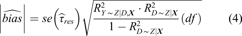
The core idea in the R² parameterization remains the same: there exists some confounder that influences the outcome and treatment take-up, and the interest is to understand how strongly that confounder needs to be related with both treatment status and the outcome to make an observed treatment effect zero. The advantage of using an R² measure is that it is scale-free, easily interpretable, and does not require distributional assumptions on how to combine multiple confounders. Using equation (4), Cinelli and Hazlett proposed several values for sensitivity analysis with an emphasis on two: the robustness value (RV) and the extreme scenario value (EV).

The robustness value

The robustness value begins by imagining the situation in which (a) the conditional association of the unobserved confounder with the treatment assignment and (b) the conditional association of the unobserved confounder with the outcome are the same. The robustness value then assesses how strong this association would have to be imply that the estimated conditional association of the treatment with the outcome in the residual regression is composed of bias to some given percentage threshold (q). When, as is typically the case, q = 100%, the robustness value RV_q = 1.0 measures how large the conditional association would have to be to imply that the estimated effect is entirely composed of bias. Formally, the robustness value starts with the proposition

R_{Y \sim Z | D, X}^{2} = R_{D \sim Z | X}^{2} \equiv R V_{q}

(5)

Using this definition of $R V_{q}$ and equation (4)

q \cdot | τ_{r e s} | \equiv | \hat{b i a s} | = s e ({\hat{τ}}_{r e s}) \sqrt{\frac{R V_{q}^{2}}{1 - R V_{q}} (d f)}

(6)

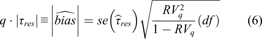
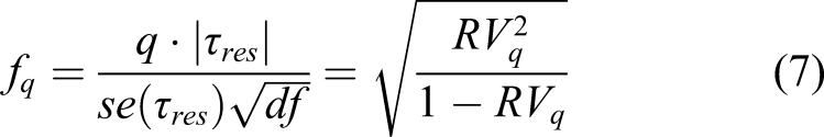
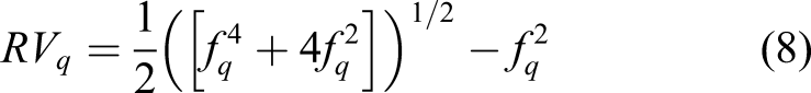
Equation (6) can be rearranged to obtain Cohen’s f, condition on X per equation (5)

f_{q} = \frac{q \cdot | τ_{r e s} |}{s e (τ_{r e s}) \sqrt{d f}} = \sqrt{\frac{R V_{q}^{2}}{1 - R V_{q}}}

(7)Solving equation (7) for RV_q

R V_{q} = \frac{1}{2} {([f_{q}^{4} + 4 f_{q}^{2}])}^{1 / 2} - f_{q}^{2}

(8)

RV_q is easy to evaluate from typical regression output and to interpret. A partial R² of, say 0.05 between a particular hypothesized but unobserved confounder and the outcome may be easy to defend, while a partial R² of 0.5 may be much more unlikely. Knowing whether the RV_q is closer to 0.05 or to 0.5 accordingly contributes substantially to the qualitative degree of confidence one can ascribe to the causal estimates.

The extreme scenario value

The extreme scenario value considers the case where a hypothetical unobserved confounder(s) explains all the remaining variance in the outcome $(R_{Y \sim Z | D, X}^{2} = 1)$ and estimates how much of the remaining variance in treatment status $(R_{D \sim Z | X}^{2})$ it would need to explain to send the estimated effect to zero. In the extreme scenario, it can be shown that when the difference-in-difference coefficient is entirely composed of bias, then the partial R² of treatment status D on the unobserved confounder Z conditional on X is equal to the partial R² of the outcome Y on treatment status D conditional on X⁵

R_{D \sim Z | X}^{2} = R_{Y \sim D | X}^{2}

(9)

Therefore, the amount of variance in the outcome explained by the treatment after accounting for the covariates, $R_{Y \sim D | X}^{2}$ , is the extreme scenario value.

The relative confounding strength value

Equation (4) also lends itself to a useful tool, the relative confounding strength (RCS) value. The RCS value considers how the estimated effect would change if there were unobserved confounders K times stronger than an observed covariate, of the researcher’s choosing. The RCS value begins by calculating how strongly related an observed confounder is with the outcome and with the treatment, and those values are then used as hypothetical stand-ins for an unobserved confounder. For example, a researcher may argue that they have controlled one of the most important confounders, X₁, and using the RCS value they estimate how the observed effect size changes if a hypothetical unobserved confounder that is K times stronger than X₁ was included in the model. The researcher can report how the estimated effect changes for different K and may find that there is some value K = k at which the estimated effect is reduced to a point such that the conclusions drawn from the study change materially.

Application to difference-in-difference models

This section applies these metrics to evaluate time-varying confounding in difference-in-difference. Calculating the robustness and extreme scenario values requires the effect estimate, the standard error, and the degrees of freedom. Utilization of the metrics is complicated by the use of cluster adjusted standard errors in difference-in-difference models because the bias formula (equation (4)) utilizes the unadjusted standard error of τ_res. We propose using a first-difference model such that cluster-adjusted standard errors are no longer required.

The first-difference model is estimated as

Δ y_{i t} = α_{0} + τ Δ D_{i t} + Δ ϵ_{i t}, t = 2,3, \dots, T

(10)where ΔD_i is the change in a time-varying treatment status and τ is the effect of interest. A first-difference estimator is used because if the error term

ϵ_{i t}

follows a random walk, then the usual standard errors are asymptotically valid.⁸ The robustness and extreme scenario values are easily estimated by hand or by using the R package, sensemakr, which can present the metrics graphically. Alternatively, if the cluster-robust standard errors are similar in value to the usual OLS standard errors, then the sensitivity metrics are also estimable without further modification to the regression.

Sensitivity metrics in practice

The application of these metrics is illustrated through two examples: the effect of Medicaid expansion under the ACA on state Medicaid spending and the effect of Medicaid expansion on Medicaid enrollment. These examples have been well studied in the literature and have easily understood policy impacts. The effect of Medicaid expansion on Medicaid enrollment is expected to be quite large and is likely to have a plausible causal interpretation. By contrast, the effect of Medicaid expansion on state spending is expected to be small because of the federal subsidy.

Effect of Medicaid expansion on state spending on Medicaid

A 2017 paper assessed the impact of Medicaid expansion on state Medicaid spending between FY 2014 and 2015.⁹ To identify the effect, the authors utilized difference-in-difference controlling for the unemployment rate and state per-capita revenue. They tested the parallel-trends assumption—in the pre-period—and found generally non-significant results which were used to support the validity of difference-in-difference. The study found non-significant and small coefficients in the difference-in-difference regression and concluded that Medicaid expansion had no statistically significant effect on state Medicaid spending.

In this example, the sensitivity metrics—robustness value, extreme scenario value, and relative confounding strength—are applied to the original analysis for the total state Medicaid spending outcome. The example reanalyzed the original data and then estimated the sensitivity analysis metrics. Following reanalysis, the example made several adjustments to the model and estimated the sensitivity analysis metrics for each adjustment.

The original model was a two-way fixed effects—state and year—model controlling for the unemployment rate and per-capita income. Table 1 reanalyzes the original model and makes three additional adjustments. The first adjustment was to remove Ohio and Connecticut from the data because a change in the way funds were reported made it impossible to disentangle federal and state spending.¹⁰ Second, the annual unemployment rate was replaced with the labor force participation rate (LFP). The LFP is a more holistic view of the job market because it includes discouraged workers who have given up looking for a job, whereas the unemployment rate only considers those who are employed or actively searching for a job. Third, a measure of state ideology was added to the model because Medicaid expansion was a divisive political issue and the states’ political ideology likely influenced both the decision to expand Medicaid as well as how each state allocates funds to the Medicaid program. Following each modification, the sensitivity metrics proposed in this paper are estimated using the sensemakr R package.

Table 1.

Modification and sensitivity analysis of Sommers and Gruber (2018).

Model	Effect	p-value	RV, %	EV, %
No controls	−7.33%	0.0384	12.52	1.76
No Ohio (OH) or Connecticut (CT)	−5.59%	0.0427	12.51	1.76
Labor force participation (LFP) + No OH or CT	−6.56%	0.0169	14.60	2.43
Ideology + LFP + No OH or CT	−6.58%	0.0147	14.92	2.55

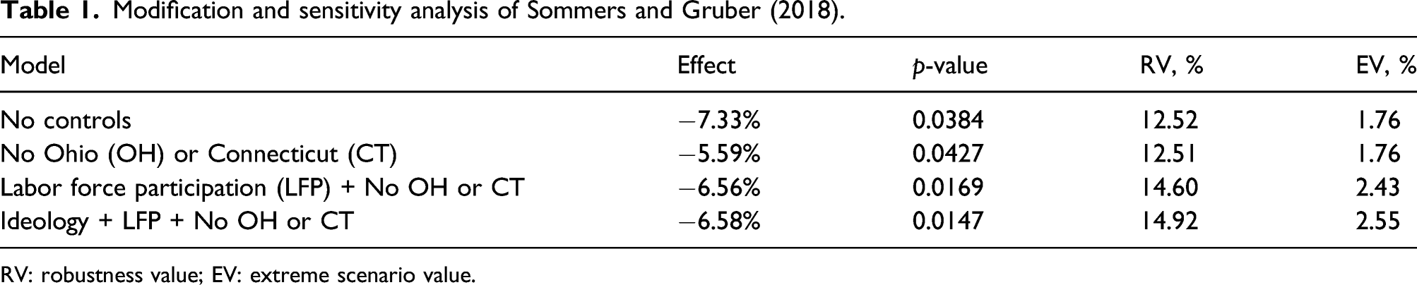
RV: robustness value; EV: extreme scenario value.

Table 1 reports the treatment effect (percent change), the p-value, and the sensitivity metrics. The sensitivity metrics were calculated using the estimated effect, standard error, and degrees of freedom from the two-way fixed effects model because the standard errors with clustering adjustment were similar to the unadjusted standard errors. With model refinements, the robustness values increased from 12.52% to 14.92%, and the extreme scenario values increased from 1.76% to 2.55%. These results can be contextualized by comparing them to the partial-R² of an important observed confounder such as the LFP. The partial-R² of the LFP with the outcome is 0.059 or 5.9%, and the partial-R² of state ideology with the outcome is 0.021 or 2.1%. If a partial-R² of 5.9% is typical for the kinds of state-level confounders that cause concern about the validity of difference-in-difference analysis of policy effects, then the concern may be assuaged. Of course, other contextual confounders may have very different partial-R² values, but this exercise at least helps to anchor expectations.

When the model controls for confounders, the relative confounding strength (RCS) value can be estimated, which expresses how much the effect changes if there were an unobserved confounder K times stronger than chosen observed confounder. In the context of Medicaid spending, the LFP rate is one of the most important confounders to control for.

Table 2 reports the RCS estimates on how the estimated treatment effect, standard error, and t-value change as the strength of a hypothetical unobserved time-varying confounder(s) increases, relative to the LFP. For example, when the strength of a hypothetical unobserved time-varying confounder(s) was four times stronger than the LFP, the estimated effect was no longer significant at the 0.05 level and decreased from the original value of −6.70% to −4.49%. Furthermore, when the strength of unobserved time-varying confounder(s) was 12 times stronger than the LFP, the estimated effect approached zero as it decreased to 0.19%.

Table 2.

Strength of unobserved confounder(s) relative to labor force participation rate and effect on estimates.

Strength of unobserved time-varying confounder(s)	Adjusted estimate	Adjusted SE	Adjusted T	Adjusted p-value
2 × LFP	−5.60%	0.026	−2.2188	0.014
4 × LFP	−4.49%	0.024	−1.9075	0.029
6 × LFP	−3.34%	0.0219	−1.5524	0.061
8 × LFP	−2.19%	0.0196	−1.1325	0.130
10 × LFP	−1.01%	0.0168	−0.6051	0.272
12 × LFP	0.19%	0.0135	0.1395	0.445

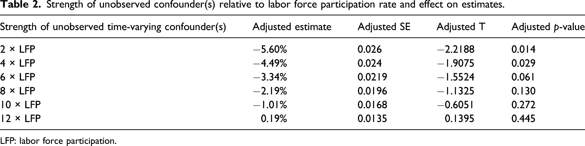
LFP: labor force participation.

Effect of Medicaid expansion on Medicaid enrollment

In 2014, the Affordable Care Act gave states the option of expanding Medicaid coverage to childless adults with incomes below 138% of the Federal Poverty Line (FPL). Following expansion of Medicaid, several studies were published investigating the effect of Medicaid expansion on Medicaid enrollment among low-income adults.^11,12 Despite variation in the data used to answer the question, each of the studies utilized difference-in-difference as the identification strategy. To justify the unbiasedness of difference-in-difference, the studies visualized and tested for the presence of parallel trends in the pre-period and found evidence in favor of the parallel trends in the pre-period.

For this example, we conducted an analysis similar to prior work but used American Community Survey data on adults with incomes below 150% of FPL. A first-difference model was used to model the effect, and the sensitivity of the results to a parallel trends violation, or time-varying confounding, was explored using the robustness value and the extreme scenario value.

The analysis found an effect of 7.64 percentage points with no control variables, which is in line with prior work^12,13 that found percentage point increases of 10.5 and 7.3. The robustness and extreme scenario values for the analysis were 55.34% and 40.68% (Table 3). The initial analysis ignored confounders such as LFP and state political ideology. Thus, it is plausible that the observed effect is partly due to changes in LFP and state ideology over time. Controlling for the LFP rate changed the effect estimate to 7.69 percentage points, slightly increased the robustness value to 55.12% and the extreme scenario value to 40.37% (Table 3). Controlling for state ideology slightly changed the effect estimate to 7.70 percentage points but increased the RV and EV values to 57.45% and 43.69%.

Table 3.

Robustness and extreme scenario values for effect of Medicaid expansion on Medicaid enrollment (percentage point change).

Model	Effect	p-value	RV, %	EV, %
Naive	7.64	<0.001	55.34	40.68
Naive + labor force participation (LFP)	7.69	<0.001	55.12	40.37
Naive + LFP + ideology	7.70	<0.001	57.45	43.69

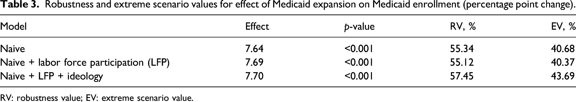
RV: robustness value; EV: extreme scenario value.

In Table 4, we estimate the RCS for a hypothetical unobserved confounder that is 1, 2, 5, and 10 times stronger than state ideology and find that the effect is robust because it remains significant despite hypothetical unobserved confounders of increasing strength. Interestingly, the treatment effect becomes more significant as the strength of the hypothetical confounder increases. The precision of the effect increases because state ideology has a very large partial-R² with the treatment and a small partial-R² with the outcome. Therefore, controlling for a hypothetical unobserved confounder that is strongly related to the treatment and negligibly related to the outcome would simultaneously increase the precision of the estimate and reduce the strength of the estimate.

Table 4.

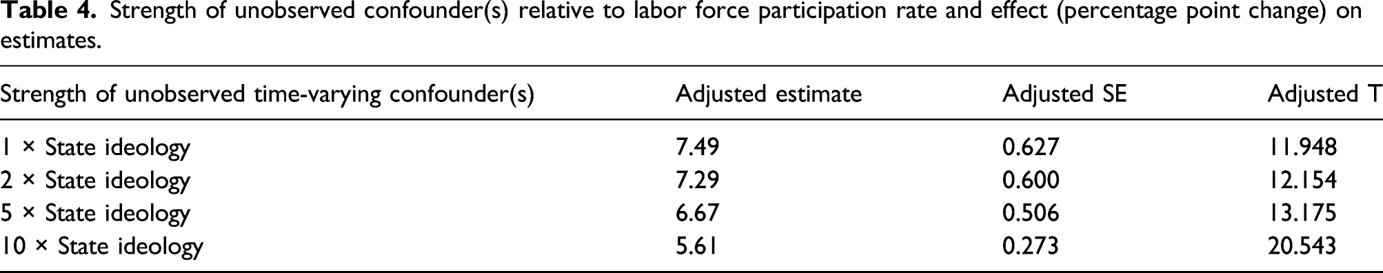
Strength of unobserved confounder(s) relative to labor force participation rate and effect (percentage point change) on estimates.

Strength of unobserved time-varying confounder(s)	Adjusted estimate	Adjusted SE	Adjusted T
1 × State ideology	7.49	0.627	11.948
2 × State ideology	7.29	0.600	12.154
5 × State ideology	6.67	0.506	13.175
10 × State ideology	5.61	0.273	20.543

A researcher might consider both state ideology and the LFP to be very important confounders that should be analyzed using the RCS values. The sensemakr package provides plots that are useful for summarizing the RCS values of multiple confounders. An example is provided below that visualizes the RCS values for both state ideology and the LFP (Figure 1).

Figure 1.

Visualizing relative confounding strength.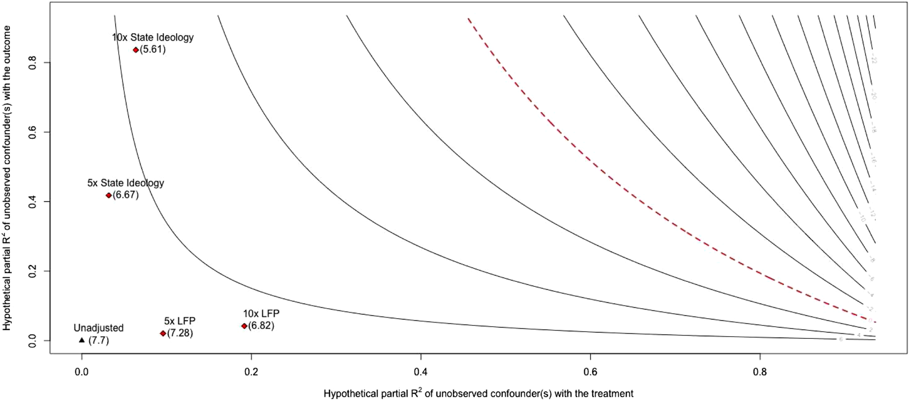

In Figure 1, each line represents the estimated effect for different values of hypothetical confounding, as measured by partial-R². The critical value, the point at which none of the estimated coefficient can be interpreted causally, is drawn by the dashed red line. The observed effect size is denoted by the black triangle in the bottom left corner when the hypothetical confounder(s) has zero relationship with either the outcome or treatment. The key elements of the plot are the red diamonds which represent the effect size given a hypothetical unobserved confounder K times stronger than the listed observed confounder. For example, when considering a confounder five times stronger than the LFP the estimated effect is 7.28, and when the hypothetical confounder is 10 times stronger than the LFP the estimated effect is 6.82.

We argue that this application may provide an approximation for the real-world upper limit of EV and RV because confounding is minimal. Plausible confounders are state finances, the LFP rate, and state ideology. State finances, however, likely have little influence on treatment uptake because the federal government covered 100% of the new costs for the first two years and 90% of the costs after. LFP does influence enrollment and states may consider LFP prior to expanding Medicaid. State ideology is likely strongly related to the decision to expand Medicaid due to the political decisiveness surrounding the topic but is questionably related to the outcome. LFP and state ideology are the two most critical confounders and as such were controlled for (Table 3).

Discussion

With these estimates in hand, a more nuanced discussion can unfold regarding the presence of time-varying confounders. For example, a reviewer may critique the paper for leaving out confounder Z. In the past, the author is limited in their ability to respond to the reviewer and must rely on arguments for why the unobserved confounder is likely of little import. With the RV, EV, and RCS estimates, however, the researcher can allow for confounder Z to be a plausible confounder and instead focus on whether confounder Z is likely strong enough to change the conclusions of the study. For the above example say that a reviewer posits the state immigration rate as an unobserved time-varying confounder. With the RV, EV, and RCS estimates, the researcher can respond by saying that state immigration rate would have to be ten times stronger than the LFP to change the conclusions of the study. Furthermore, the state immigration rate would need to have a partial-R² of at least 14.92% with both the outcome and the treatment to send the effect to zero, which seems unlikely given that LFP has the highest observed partial-R² of 5.69%.

The range of examples discussed above provide a starting point for evaluating the continuum of values the EV and RV measures may take. The Medicaid enrollment example (RV = 57%, EV = 44%) likely provides us with a feasible upper limit for the robustness and extreme scenario values in real-world applications. The Medicaid spending example represents results from a study where interpretation of the EV and RV is difficult but presents the RCS values and partial R² for observed confounders as ways to contextualize the results.

We recommend that the sensitivity metrics are used for evaluating the strength of the evidence, on a continuum, for the conclusions drawn from a difference-in-difference model. While one may be tempted to create a threshold for the EV, RV, or RCS measures, doing so would defeat the purpose and intent of the sensitivity metrics. The sensitivity metrics should be used to understand how robust the effect estimate is to unobserved confounding and to promote discussion as to whether confounder(s) exist with enough strength to change the conclusions of the study.

These tools should not be used as a measure for model selection. This would result in a biased effect because the metrics are not identifying confounders and controlling for them; expert content knowledge is required to properly identify confounders. Models should be selected based on an identification strategy that seeks to make treatment assignment independent of the outcome. In the second example, we did not select our model based on the EV and RV, but instead sought to highlight how the EV and RV change as we make purposeful modifications to the model based on a causal structure.

Similar advancements in this field are the E-value, proposed by Vanderweele and Ding (2017)⁶ and the R_max and $δ_{o s t e r}$ parameters proposed by Oster.⁷ The E-value is a sensitivity measure specifically for the risk ratio that, when applied to other effect measures, is an approximation. Comparatively, if linear regression is used to obtain an effect estimate—as may be the case when using a first-difference, difference-in-difference model – the robustness values proposed in this paper are not approximations. As discussed in detail in Cinelli and Hazlett (section 6.3), Oster’s parameters are difficult to interpret and may be mis-interpreted in practice because they do not have direct analogs to better understood statistical summary measures such as correlation and covariance.⁵ Which measure is preferable largely depends on context, but it is important that researchers are aware of alternative options.

The sensitivity metrics are a valuable addition to the social scientist’s toolbox when making causal inferences with difference-in-difference. The metrics can be estimated in R or Stata using the sensemakR package. The metrics quantify how much unobserved confounding the estimated effect, or statistical significance of the estimated effect, can handle before the conclusions change. Furthermore, the metrics can be used in conjunction with observed confounders to contextualize the sensitivity values. Combined with expert content knowledge, we hope the sensitivity metrics can create a more nuanced discussion between researchers about how unobserved confounding impacts causal results by providing quantitative guidelines for how sensitive causal effects from difference-in-difference are to unobserved confounding.

Difference-in-difference relies on the assumption that no time-varying confounding remains in order for the causal effect to be identified, known as the parallel trends assumption. Unfortunately, in health policy it is often infeasible to measure every confounder. Traditional methods for assessing the parallel trends assumption arbitrate only whether or not parallel trends holds in the periods prior to treatment. In addition, indirect parallel trends tests result in binary verdicts that ignore the relationship between the magnitude of a parallel trends violation and the estimated effect. This paper contributes to the difference-in-difference literature by extending a suite of sensitivity analysis metrics to analyze how sensitive a causal estimate from difference-in-difference is to unobserved time-varying confounding, or parallel trends violations, on a continuum.

Footnotes

Declaration of conflicting interests

The author(s) declared no potential conflicts of interest with respect to the research, authorship, and/or publication of this article.

Funding

The author(s) disclosed receipt of the following financial support for the research, authorship, and/or publication of this article: This work was supported by the Agency for Healthcare Research and Quality.

ORCID iD

Landon Gibson

References

Ryan

Burgess

Dimick

. Why we should not be indifferent to specification choices for difference-in-differences. Health Serv Res 2015; 50(4): 1211–1235. DOI: 10.1111/1475-6773.12270.

Cornfield

Haenszel

Hammond

, et al. Smoking and lung cancer: recent evidence and a discussion of some questions. JNCI: J Natl Cancer Inst 1959; 22(1): 173–203. DOI: 10.1093/jnci/22.1.173.

Rosenbaum

. Sensitivity analysis for certain permutation inferences in matched observational studies. Biometrika 1987; 74(1): 13–26. DOI: 10.1093/biomet/74.1.13.

Rosenbaum

. Sensitivity analysis for matching with multiple controls. Biometrika 1988; 75(3): 577–581. DOI: 10.1093/biomet/75.3.577.

Cinelli

Hazlett

. Making sense of sensitivity: extending omitted variable bias. J Royal Stat Soc Ser B (Statistical Methodology) 2020; 82(1): 39–67. DOI: 10.1111/rssb.12348.

VanderWeele

Ding

. Sensitivity analysis in observational research: introducing the E-value. Ann Intern Med 2017; 167(4): 268. DOI: 10.7326/M16-2607.

Oster

. Unobservable selection and coefficient stability: theory and evidence. J Business Econ Stat 2019; 37(2): 187–204. DOI: 10.1080/07350015.2016.1227711.

Wooldridge

. Introductory Econometrics: A Modern Approach. 2nd ed. Australia, Cincinnati, Ohio: Southwestern College Pub, 2003. ISBN 978-0-324-11364-8.

Sommers

Gruber

. Federal funding insulated state budgets from increased spending related to medicaid expansion. Health Aff 2017; 36(5): 938–944. DOI: 10.1377/hlthaff.2016.1666.

10.

Potamianos

Cohen

Kelly

, et al. 2018 State expenditure report - fiscal years 2016 to 2018. Technical report, National Association of State Budget Officers, 2018.

11.

Kaestner

Garrett

Chen

, et al. Effects of ACA medicaid expansions on health insurance coverage and labor supply. J Policy Anal Manage 2017; 36(3): 608–642. DOI: 10.1002/pam.21993.

12.

Wherry

Miller

. Early coverage, access, utilization, and health effects associated with the affordable care act medicaid expansions: a quasi-experimental study. Ann Intern Med 2016; 164(12): 795. DOI: 10.7326/M15-2234.

13.

Decker

Lipton