
Abstract
Selection bias is a common type of bias, and depending on the causal estimand of interest and the structure of the selection variable, it can be a threat to both external and internal validity. One way to quantify the maximum magnitude of potential selection bias is to calculate bounds for the causal estimand. Here, we consider previously proposed bounds for selection bias, which require the specification of certain sensitivity parameters. First, we show that the sensitivity parameters are variation independent. Second, we show that the bounds are sharp under certain conditions. Furthermore, we derive improved bounds that are based on the same sensitivity parameters. Depending on the causal estimand, these bounds require additional information regarding the selection probabilities. We illustrate the improved bounds in an empirical example where the effect of breakfast eating on overweight is estimated. Lastly, the performance of the bounds are investigated in a numerical experiment for sharp and non-sharp cases.
Introduction
In observational studies, there are several sources of potential biases when estimating a causal effect of an exposure on an outcome of interest. One type of bias in observational studies is selection bias which can occur when the study is conducted in a subset of a population. Intuitively, selection bias can arise when the target population is the total population, that is, one wishes to generalize the results to subjects in both the selected and non-selected part of the population. However, selection bias can also arise when the target population is the selected part of the population. Commonly, when no inclusion criteria are employed, the estimand of interest lies in the total population, and when inclusion criteria are used, the interest instead often lies in the subpopulation estimand. To assess the maximum magnitude of the potential selection bias, a sensitivity analysis can be used, e.g. calculating bounds for the causal estimands under selection bias. Several analytical bounds have been proposed, both for total population estimands and subpopulation estimands.1–5 Alternatively, Duarte et al. 6 propose an algorithm for deriving numerical bounds.
Here, we build upon Smith and VanderWeele, 7 hereafter referred to as SV. These authors developed bounds that require the analyst to specify certain sensitivity parameters under specific conditional independence assumptions. The sensitivity parameters describe the maximum strength of the dependence between the selection variable, the outcome, the exposure and an unmeasured variable. However, SV did not discuss whether the sensitivity parameters are variation independent of each other and the observed data distribution. This is a desirable property since the sensitivity parameters can be specified individually without taking the value of the other sensitivity parameters into account. Furthermore, SV did not discuss whether their bounds are sharp relative to the necessary assumption and information when the sensitivity parameters and data distribution fulfill specific criteria. In this work, we investigate the SV bounds in similar ways as Sjölander 8 did for bounds for causal estimands under confounding. More specifically, we derive the feasible regions of the sensitivity parameters and show that they are variation independent of each other and the observed data distribution, and we show that the SV bounds are sharp under specific criteria, that is, they are the tightest possible bounds under the necessary assumptions, and that they are non-sharp when the criteria are not fulfilled, that is, tighter bounds can be found. Furthermore, we propose improved sharp bounds using the same sensitivity parameters as the SV bounds, noting that they require additional knowledge of the data in some instances. The improved bounds coincide with SV’s bounds in certain areas and are tighter in others. The bounds and how they can be used are illustrated in an empirical example investigating the causal effect of breakfast-eating on overweight. The performance of the bounds in comparison to the SV bounds are evaluated in a numerical example. Here, we show that the improved bounds are typically tighter when the additional knowledge is used, but that the two bounds are similar when the additional knowledge is not used.
The rest of the article is structured as follows. In Section 2, we present notation, definitions, and assumptions and briefly report SV’s bounds. In Section 3, we derive the theoretical properties of the SV bounds and present the improved bounds in Section 4. We illustrate the improved bounds in an empirical example and numerical example in Sections 5 and 6, and finally, discuss the results in Section 7.
Theoretical framework
Notations, definitions, and assumptions
Notation is presented in throughout in the text, and a summary is found in Supplemental Appendix A. We use the Neyman-Rubin causal model9,10 to define potential outcomes,

If the interest lies in the total population, that is, the target is to generalize the results to subjects in both the selected and non-selected part of the population, the target estimand is


On the other hand, if the specific subpopulation is of interest, that is, the target is to generalize the results only to subjects in the selected part of the population, the target estimand is instead

We caution the reader that Assumption (4) for the selected subpopulation is more subtle than the corresponding Assumption (2) for the total population, and that there are realistic situations where, for a given set of variables
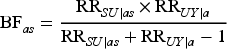
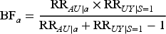
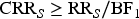
In this work, selection bias is measured on the same scale as the estimand, so for the risk ratios the bias is defined as
The effect of breakfast-eating on body mass index (BMI) has previously been studied using the National Health and Nutrition Examination Survey (NHANES) data, 1999-2000, and Song et al.
11
studied whether skipping breakfast is associated with BMI in US adults. Here, we use this example to illustrate the assumptions and bounds using NHANES data from 1999 to 2018.
12
The original article includes several covariates in the analysis, but we focus on one stratum in line with the setting of this article. The stratum considered is reliable responders, men, 30–39 years old, non-hispanic white, non-smokers, and non-exercisers. Furthermore, marital status can be considered to be a proxy variable for other variables that may be correlated with breakfast eating and/or overweight and are more difficult to quantify, for example, socioeconomic status and lifestyle habits. If a selection on marital status is made, and only subjects who are married/living with a partner are included, one might think that the bias is reduced (Figure 1(a)) when instead marital status is not a confounder, and the bias is increased due to selection bias from a potential M-structure (Figure 1(b)). Here, the unknown variable
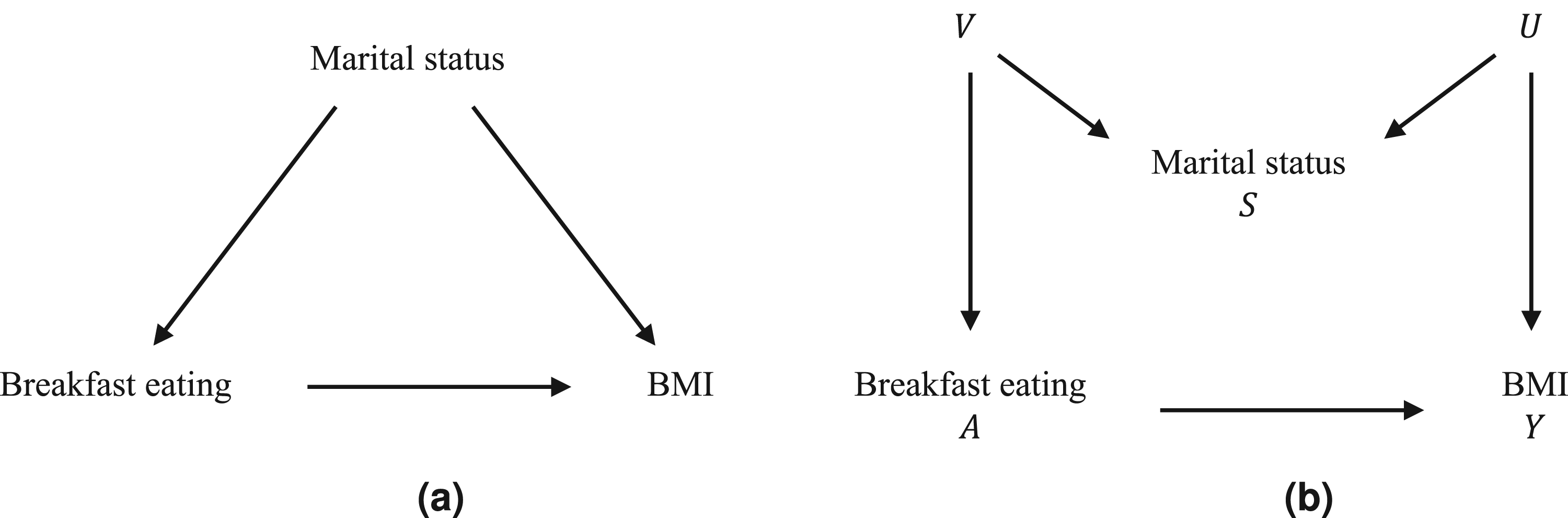
Possible structures for the selection where (a) marital status is a confounder and (b) a collider.
The sensitivity parameters in the SV bounds are constructed as risk ratios that describe the maximum strengths of dependencies between the unmeasured variable U in relations (2) to (4), and the other variables. For the total population, SV defined the sensitivity parameters as follows:
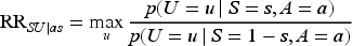
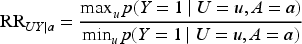
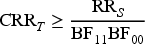

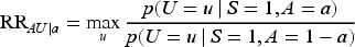
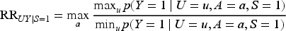

The sensitivity parameters measures the potential magnitude of the maximum selection bias. If no selection bias is present, they are equal to 1. Interpretations of the sensitivity parameters have previously been discussed.
5
In terms of the NHANES example, the sensitivity parameters
SV only presented lower bounds, both in the total and subpopulation, and they suggested that the exposure variable should be recoded when the upper bound is of interest. To simplify for the data-analysts, we have constructed an upper bound that is equal to the lower bound with the recoded exposure.
Properties of SV’s bounds
Feasible regions
It is desirable to set sensitivity parameters to values that are logically possible based on their definitions. Thus, we start with deriving the sets of logically possible values for the sensitivity parameters, that is, their feasible regions. Sensitivity parameters can be restricted by, for example, the data, their definitions or by each other. If a sensitivity parameter is not restricted by another quantity, then it is said to be variation independent of that quantity. Variation independence is desirable because it simplifies for user as the sensitivity parameters can be considered separately. Theorem 1 considers feasible regions and variation independence for the sensitivity parameters for the total population:
The reason for caring about variation independence of
Theorems 1 and 2 imply that the users of the bounds can consider all values >1 as logically possible, although they might not be equally plausible. The proofs of Theorems 1 and 2 are given in Supplemental Appendices D and E. See Chen,
13
Nabi et al.,
14
Malinsky et al.,
15
Shpitser
16
for results on variation independent parameters in other settings. Note that it is enough to show variation independence for one specific distribution because that means that there exists (at least) one unmeasured variable
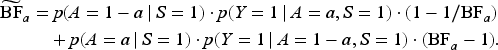
A bound is valid if it contains the true causal estimand. Furthermore, a bound is sharp if the bias can be equal to the value of the bound, for an observed distribution and correctly specified sensitivity parameters. Thus, a sharp bound is the tightest valid bound. Bounds are derived under specific assumptions and information, and a bound is thus sharp under its necessary assumptions and information. Thus, two different bounds for the same causal estimand can be simultaneously sharp if they are derived under different assumptions and information. We emphasize that a bound can be valid even though it is not sharp.
The SV bounds for the risk ratio in the total population are sometimes arbitrarily sharp, in the sense that the selection bias can be arbitrarily close the bound, but not exactly equal. More details are given in Supplemental Appendix F. In Theorem 3, we present sufficient conditions for when the SV bounds for the risk ratio in the total population are arbitrarily sharp. Theorem 3 is proved in Supplemental Appendix F.
Given Assumptions (1)–(3) and
Given Assumptions (1)–(3) and
Thus, if
The lower SV bound for the risk difference in the total population is generally not sharp, except for the very specific condition
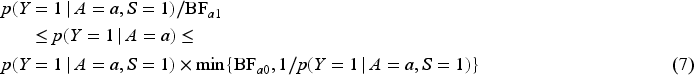
The SV bounds for the risk ratio in the subpopulation are sometimes sharp. In Theorem 4, which is proved in Supplemental Appendix G, we present a necessary and sufficient condition for when the SV bounds for the risk ratio in the subpopulation are sharp.
Given Assumptions (1) and (4) and
Given Assumptions (1) and (4) and
Thus, if
The SV bounds for the risk difference in the subpopulation are arbitrarily sharp. Sufficient and necessary conditions are presented in Theorem 5, proved in Supplemental Appendix H.
Given Assumptions (1) and (4) and
Given Assumptions (1) and (4) and
Thus, if

A consequence of the results on sharpness is that one can obtain improved bounds, that is, bounds that are equal to the SV bounds when they are sharp and tighter in the region where the SV bounds are not sharp. Such bounds are presented in the next section.
Total population
The SV bounds in the total population are not sharp under certain conditions, as shown in the previous section, but the sensitivity parameters can be used to construct improved bounds that are generally sharp. Define


The bounds The bounds The bounds
To be able to use these bounds in practice, one must know, or have a reasonable guess, the sampling proportion

The lower bound and upper bounds in (6) are monotonically decreasing and increasing in
The SV bounds in the subpopulation are only sharp under specific conditions, as shown in the previous section, but the sensitivity parameters can be used to construct improved bounds that are generally sharp. We define

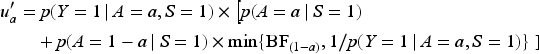

The bounds The bounds The bounds
A result of Theorem 7 is that one can construct sharp lower (upper) bounds for any contrast between
Here, we demonstrate the improved bounds by revisiting the NHANES example where the effect of breakfast-eating on overweight (BMI>25) using NHANES data from 1999 to 2018 is investigated.
12
The original article includes several covariates in the analysis, but we analyze one stratum in line with the setting of this article. If more strata are of interest, the sensitivity analysis will have to be repeated in each stratum. There are 576 subjects in the chosen stratum where 436 subjects are selected (married or living with a partner). Among all subjects (selected and non-selected), 473 are breakfast eaters, and 103 are breakfast skippers. Among the selected subjects, 371 eat breakfast and 65 do not eat breakfast. Among the selected breakfast eaters, 239 subjects are overweight, and among the selected breakfast skippers, 53 are overweight. Thus, we obtain
The contour plot in Figure 2(a) shows values of
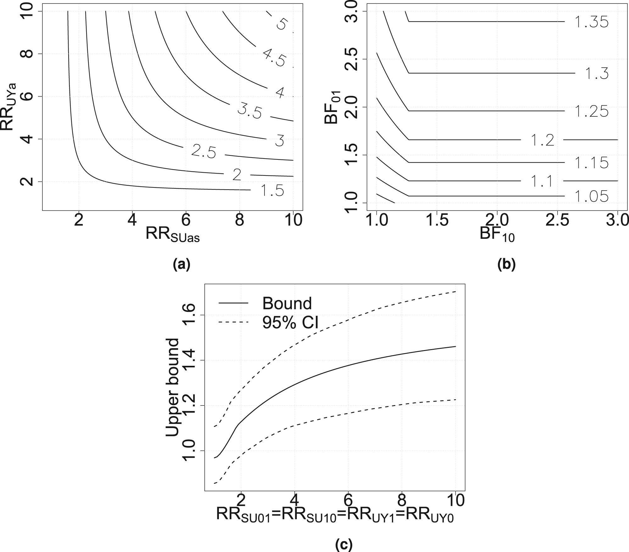
Contour plots for (a)
Sampling variability should also be considered when calculating the bounds, since the probabilities are estimated. Here, we apply a nonparametric bootstrap resampling procedure. The probabilities used in the calculations of the bounds are sampled from binomial distributions where the parameters are taken from the data. A total of 1000 bootstrap samples are taken and the bounds are calculated. 95% confidence intervals for the upper bounds when the sensitivity parameters are assumed to be equal are calculated as the 0.025 and 0.975 quantiles for the bootstrap samples. The bounds and 95% point-wise confidence intervals are shown in Figure 2(c). The confidence intervals are fairly wide. The uncertainty is partly due to the relatively small sample size in the breakfast-skipping group. Furthermore, additional uncertainty that comes from generalizing the conclusions to the non-selected part of the population as well.
Similarly, in Figure 3(a), the upper bound
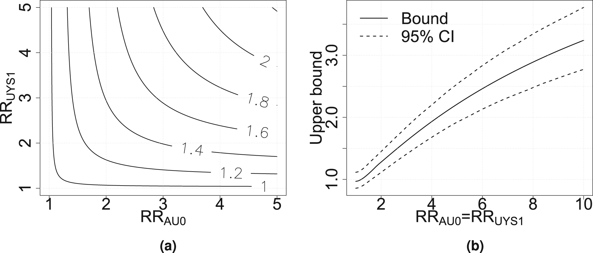
Contour plot for (a) the upper bound for
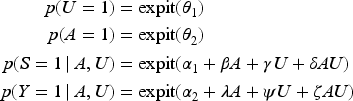
The performance of the SV and improved bounds for all four estimands are compared in a numerical example. The distributions are generated from the causal model in Figure 4 where Assumptions (2) to (4) hold. The model is parameterized as follows:
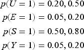
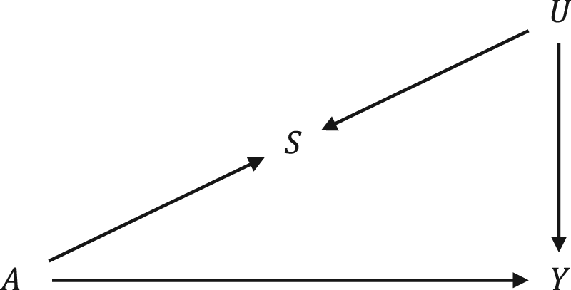
Structure of the data-generating process in the numerical example.
The setup results in 32 combinations of probabilities and standard deviations. For each combination, 1000 distributions are generated, and for each distribution, the causal estimand, the observed estimand, and the SV and improved lower and upper bounds are calculated using the true probabilities. For the total population estimands, the alternative bounds which sets
In Table 1, the results for the sharp bounds for the risk ratio in the total population are presented. Here,
Results for
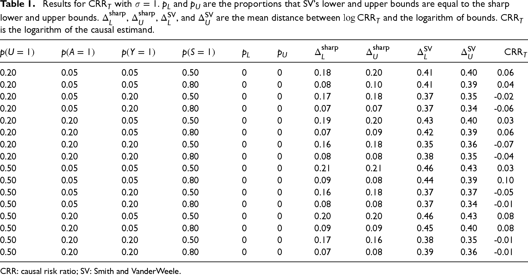
CRR: causal risk ratio; SV: Smith and VanderWeele.
Results for
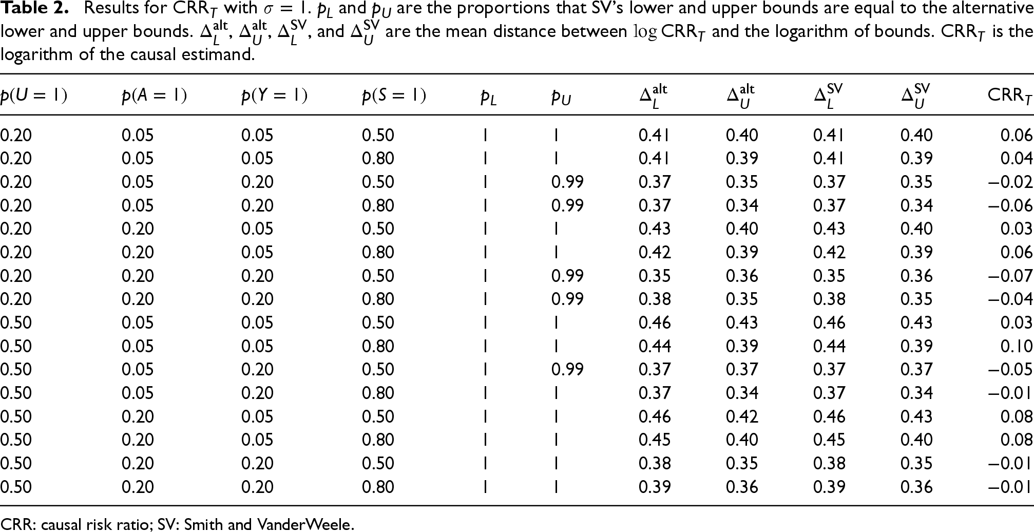
CRR: causal risk ratio; SV: Smith and VanderWeele.
The results for the sharp bounds for the risk difference in the total population are similar to the risk ratio, see Table 3. The SV bounds for the risk difference in the total population are rather conservative, and these results are in line with previous results.
18
Here,
Results for
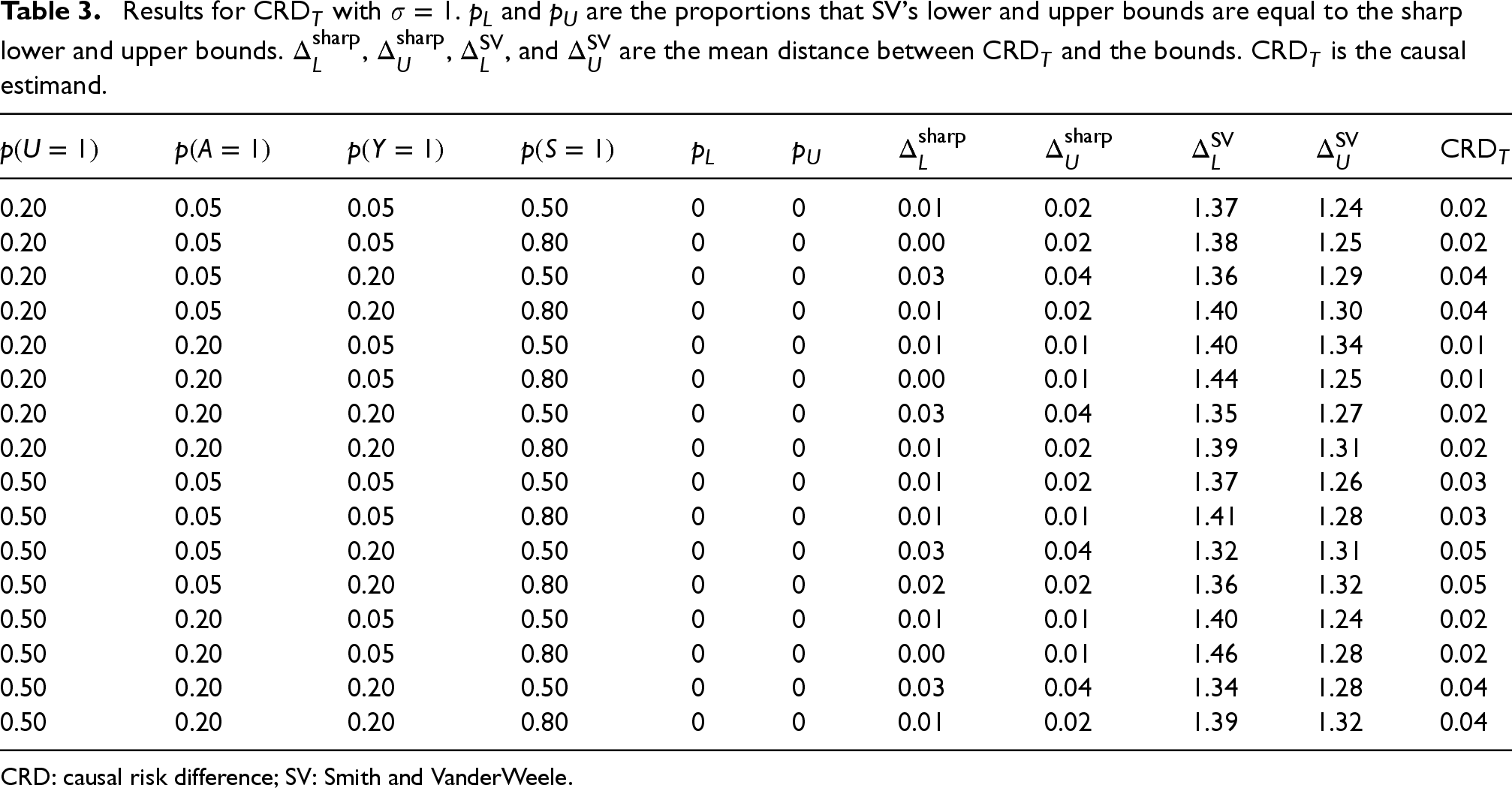
CRD: causal risk difference; SV: Smith and VanderWeele.
Results for
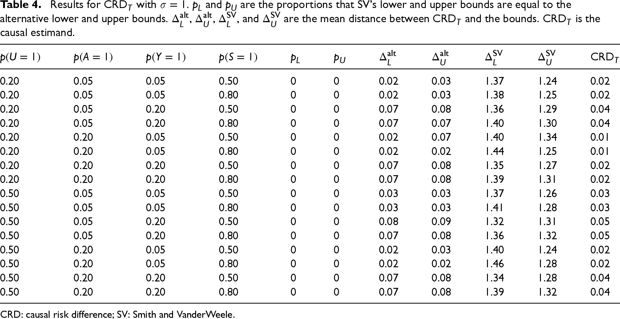
CRD: causal risk difference; SV: Smith and VanderWeele.
For the risk ratio in the subpopulation, Table 5, the results are very different. Here, the SV bounds are always equal to the sharp bounds and
Results for
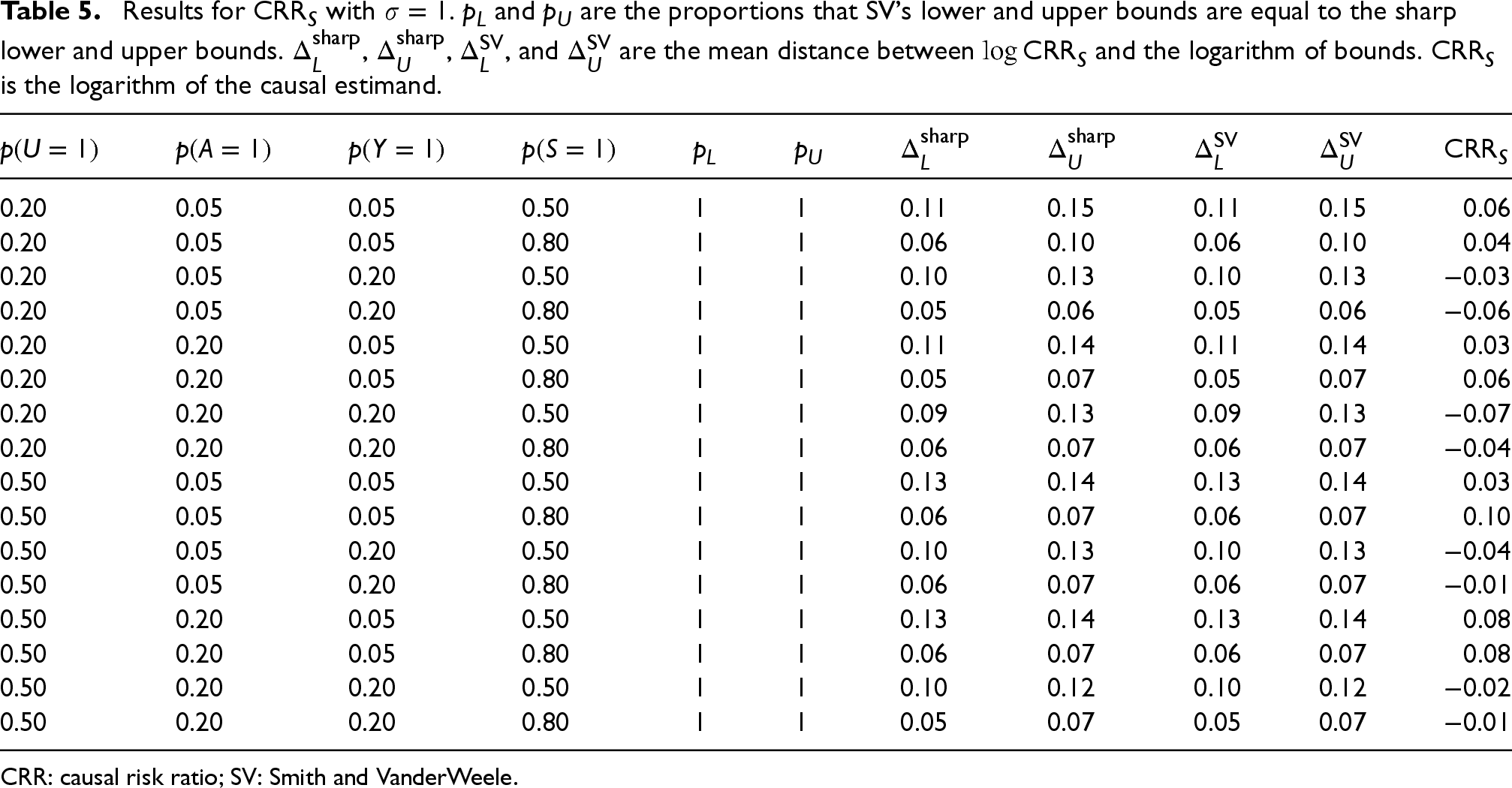
CRR: causal risk ratio; SV: Smith and VanderWeele.
Results for
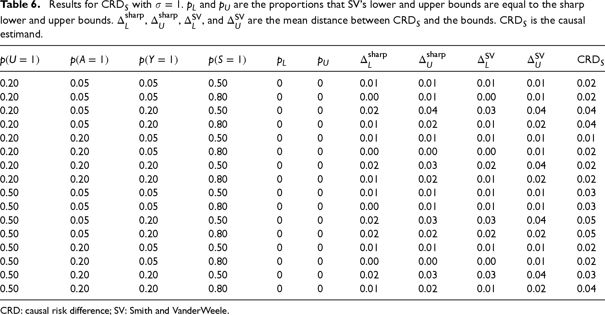
CRD: causal risk difference; SV: Smith and VanderWeele.
The results for
Bounds for bias are one type of sensitivity analysis. Here, we add to the literature on bounds for causal estimands under selection bias in similar ways as Sjölander 8 did for bounds for causal estimands under confounding. First, we have derived new properties of the previously proposed SV bounds. We have shown that the sensitivity parameters are variation independent, which is important when considering which values to set the sensitivity parameters to. Furthermore, we have also investigated the sharpness of the SV bounds. The SV bounds are sharp under certain conditions for the data distribution and sensitivity parameters, some of which are more likely to be fulfilled than others.
Since the SV bounds are only sharp under certain conditions, improved bounds can be derived. Using the same sensitivity parameters, we have derived improved bounds which are sharp. The bounds for the causal estimands in the total population require additional information on the selection probability compared to the SV bounds. In some studies, for example, register-based studies where data is available on all subjects, including the non-selected ones, these probabilities are available. In other studies, they are unknown. If this knowledge is not available, alternative bounds can be calculated by setting these probabilities to zero. The alternative bounds are equal to the SV bounds in some regions and tighter in others. The improved bounds for the causal estimands in the subpopulation is simply the minimum value of the SV bound and the sharp limit. Thus, the improved bounds are equal to the SV bounds when the latter are in the sharp region and tighter when they are not.
There are some limitations to the bounds presented here. The sensitivity parameters of the bounds are defined as ratios between the maximum and minimum of conditional probabilities. In the case of many selection variables, as is not uncommon in practical studies, the sensitivity parameters can get very large, which results in bounds that too conservative to give any information about the size of the bias. Furthermore, the results in this article are derived given fixed values of the sensitivity parameters. Determining a reasonable range of the sensitivity parameters by calibrating them against observed quantities is an important but technically difficult topic for future research. Lastly, the bounds are derived under the assumption of no unmeasured confounding. However, it is possible that a study suffers from several types of biases. An important contribution would therefore be a sensitivity analysis that takes multiple types of biases into account.
Supplemental Material
sj-pdf-1-smm-10.1177_09622802251374168 - Supplemental material for Investigations of sharp bounds for causal effects under selection bias
Supplemental material, sj-pdf-1-smm-10.1177_09622802251374168 for Investigations of sharp bounds for causal effects under selection bias by Stina Zetterstrom, Arvid Sjölander and Ingeborg Waernbaum in Statistical Methods in Medical Research
Footnotes
Consent to participate
Consent for publication
Not applicable.
Data availability statement
Declaration of conflicting interest
The author(s) declared no potential conflicts of interest with respect to the research, authorship, and/or publication of this article.
Ethical considerations
The example data in this article comes from the NHANES study, which declares the following ethical statement. The National Center for Health Statistics (NCHS) Ethics Review Board (ERB) ensures that research involving human participants protects the rights and welfare of study participants and conforms to U.S. federal regulations. The NCHS ERB, and the formal review bodies that preceded it, have approved each NHANES study protocol since the survey began running continuously in 1999. Before that, different procedures ensured the protection of human participants. Information on the ethical review board decision for the NHANES study used in this article can be found on ![]() .
.
Funding
The author(s) disclosed receipt of the following financial support for the research, authorship, and/or publication of this article: The work was funded by Swedish Research Council, grant numbers 2016-00703 and 2020-01188.
Supplemental material
Supplemental material for this article is available online.
References
Supplementary Material
Please find the following supplemental material available below.
For Open Access articles published under a Creative Commons License, all supplemental material carries the same license as the article it is associated with.
For non-Open Access articles published, all supplemental material carries a non-exclusive license, and permission requests for re-use of supplemental material or any part of supplemental material shall be sent directly to the copyright owner as specified in the copyright notice associated with the article.