Grade control drillhole spacing and mining selectivity determination using high resolution simulations applied on distinctly heterogeneous open pit mines

Abstract

The grade control drillhole spacing and mining selectivity decisions are typically made using the resource model estimated from exploration and infill drilling data. Once production starts, large quantities of grade control data are collected to delineate ore and waste boundaries for ore control. In this work, a grade control drillhole spacing and mining selectivity optimization workflow is presented which allows the practitioner to use site specific knowledge to determine the most profitable ore control mining scenario. The densely gridded production data is used to simulate a ground truth block model from which scenarios of variable drillhole spacing and selectivity are evaluated against their corresponding costs to determine the maximum profit scenario. Eleven mining scenarios are evaluated using year production data from three distinctly heterogeneous mine with drillhole spacing and mining selectivity varying from 3 × 3 × 3 m (27 m³) to 30 × 30 × 15 m (13,500 m³). The profit differences from the optimum scenario varied by millions of dollars (1–8%) against the next best case depending on the heterogeneity of the deposit. Practitioners could apply this workflow to inform grade control drillhole spacing and mining selectivity decisions for different domains within the mine or multiple pits especially if distinctly heterogeneous volumes exist.

Introduction

To confirm the potential discovery of an economic deposit, a considerable amount of infill drilling is conducted to confidently estimate the resources and reserves typically summarized in a feasibility study. Various studies have focused on optimizing the drillhole density for resource modeling, typically aimed at achieving a confidence requirement for public disclosure of resource and reserves (Rossi and Deutsch, 2013). Most of the drillhole spacing optimization workflows tend to follow the same general approach of using previous data to simulate a ground truth from which drillhole samples are drawn at various spacings, estimated, and evaluated against the simulated grades and corresponding drilling costs. While the inputs and outputs are similar, various distinct methodologies have been developed, each tailored to solve a different aspect of the optimal drillhole spacing problem.

Despite optimizing the same drillhole spacing parameter, Afonseca and Miguel-Silva (2022) demonstrate how various studies define the objective function differently using distinct metrics to capture estimation error, stochastic uncertainty, or financial gains. Englund and Heravi (1993) minimized the misclassification rate of the estimated model against the conditionally simulated truth while Li et al., (2004) measured the relative absolute error to determine the drillhole spacing required to achieve a certain level of confidence. Koppe et al. (2011), Usero et al., (2019), and Drumond et al., (2020) all minimized uncertainty using quantile ranges standardized by the average of various simulations following methodology originally proposed by Verly et al., (2014). Boucher et al., (2005) was among the first drillhole optimization studies to maximize profit which is harder to do as several unknown variables exist during the resource modeling stage. While determining the best optimization metric for resource and reserve infill drilling is complex, when considering grade control drillhole spacing for a producing mine the all-encompassing profit metric is the best to optimize for since at the extraction stage all the relevant parameters are better known (Gomes, 2023).

Many crucial mine design decisions such as the grade control drilling density, mining selectivity, and mining equipment are made with the resource model. Even after a confident estimate is made, mines encounter unexpected grades and tonnages from the resource model especially for more heterogeneous orebodies demonstrated by various reconciliations studied by Parker (2012) and synthetic examples by Journel (2018). Changes to mine design after production has started are more difficult but can be practically achieved and later improved with little additional cost or if the right hybrid equipment is in place (Groeneveld et al., 2012; Parker, 2012). Once extraction starts, grade control production is adequate for defining ore and waste boundaries in short range mine planning but after a volume is mined out, the data is not often used to make better ore control decisions in future pushbacks of similar surrounding pits (Froyland et al., 2018; Li et al., 2021; Ruiseco and Kumral, 2017).

When mines begin extraction of the orebody, large quantities of production data are used for short range mine planning and ore control. Obtaining the grade control data is important for minimizing dilution and ore loss (Abzalov et al., 2010; Harding and Deutsch, 2022) but the drilling costs and utilization can be a significant component in the overall costs for mine operations (Abbaspour et al., 2018; Boucher et al., 2005; Ugurlu, 2019). Establishing the drillhole spacing and mining selectivity is an important decision which can significantly enhance or detract from the profitability of a mine (Chiquini and Deutsch, 2020; Jara et al., 2006). Published studies regarding drillhole spacing analysis and determining the selective mining unit (SMU) have been limited in scope to resource modeling using exploration and infill drilling data and it is not until recent years that studies using production data for similar workflows have started (Gomes, 2023). There has not been much published work on the use of production data to optimize drillhole spacing for short range grade control and the influence of heterogeneity and variable mining selectivity as an input has not been tested.

Heterogeneity is an important consideration in the balance of increasing the drilling density to obtain more samples for defining a more selective mining unit versus reducing drilling cost and ore control efforts to maintain a low operating cost (Dagasan et al., 2019; Smith et al., 2014). Grade control is more challenging in more variable deposits and when operated at the same selectivity as a more homogeneous deposits they will likely have higher degrees of ore loss and dilution as illustrated in Figure 1 (Faraj, 2024; Li et al., 2021). The influence of deposit heterogeneity has not been directly studied under the same drillhole spacing analysis workflow for short range grade control but likely has a significant on the optimal result (Figure 1).

Figure 1.

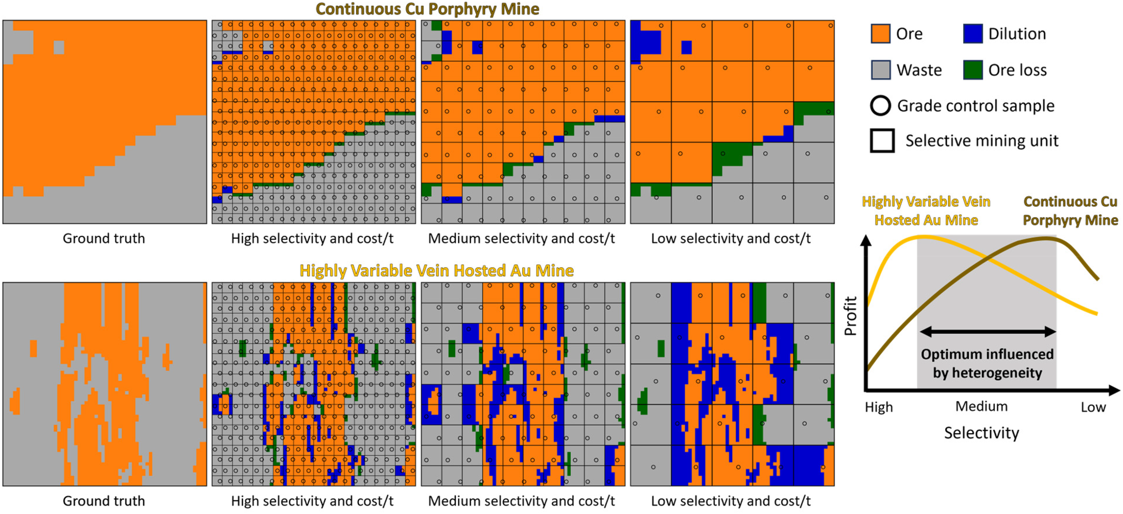
Schematic showing how the profit is maximized at lower selectivity and cost/t for a continuous Cu porphyry mine which is subject to less dilution and ore loss compared to a highly variable Au mine.

In summary, this paper seeks to establish a drillhole spacing and mining selectivity optimization workflow which allows the practitioner to define the profit using various site-specific inputs under multiple mining scenarios. The workflow expands on previous drillhole spacing studies by incorporating variable selectivity and heterogeneity from different deposits with applications for short range grade control rather than resource estimation. Drillhole spacing and mining selectivity optimization workflow describe the optimization methodology for testing different drillhole spacings and mining selectivity on a simulated high-resolution block model. Application on distinctly heterogeneous open pit mines applies the drillhole spacing and mining selectivity optimization workflow on block models simulated using one year production data from three mines: a continuous Cu porphyry, an iron oxide copper gold (IOCG) deposit, and a highly variable vein hosted Au mine. Value driving variables impacting the optimization are discussed in Workflow potential and limitations with recommendations for practitioners seeking to determine ideal grade control drilling density and mining selectivity. The conclusions of this work are presented in conclusions with directions for future work.

Drillhole spacing and mining selectivity optimization workflow

The proposed methodology allows the practitioner to define custom input parameters and grade control data for any open pit deposit to determine the optimal drillhole spacing and mining selectivity. The grade control data is used to simulate a ground truth block model from which drillhole samples are drawn at the predefined grids to estimate into their corresponding SMU sizes. The SMU grades are then compared to the true simulated grades to determine the optimal drillhole spacing and mining selectivity by quantifying the profit of each scenario (Figure 2). The workflow maximizes the profit so careful consideration is required to capture all relevant economic, operational, geological, and metallurgical variables into economic functions. Part of capturing all relevant details to maximize the profitability of the grade control mining stage includes quantifying the negative impact of dilution and ore loss.

Figure 2.

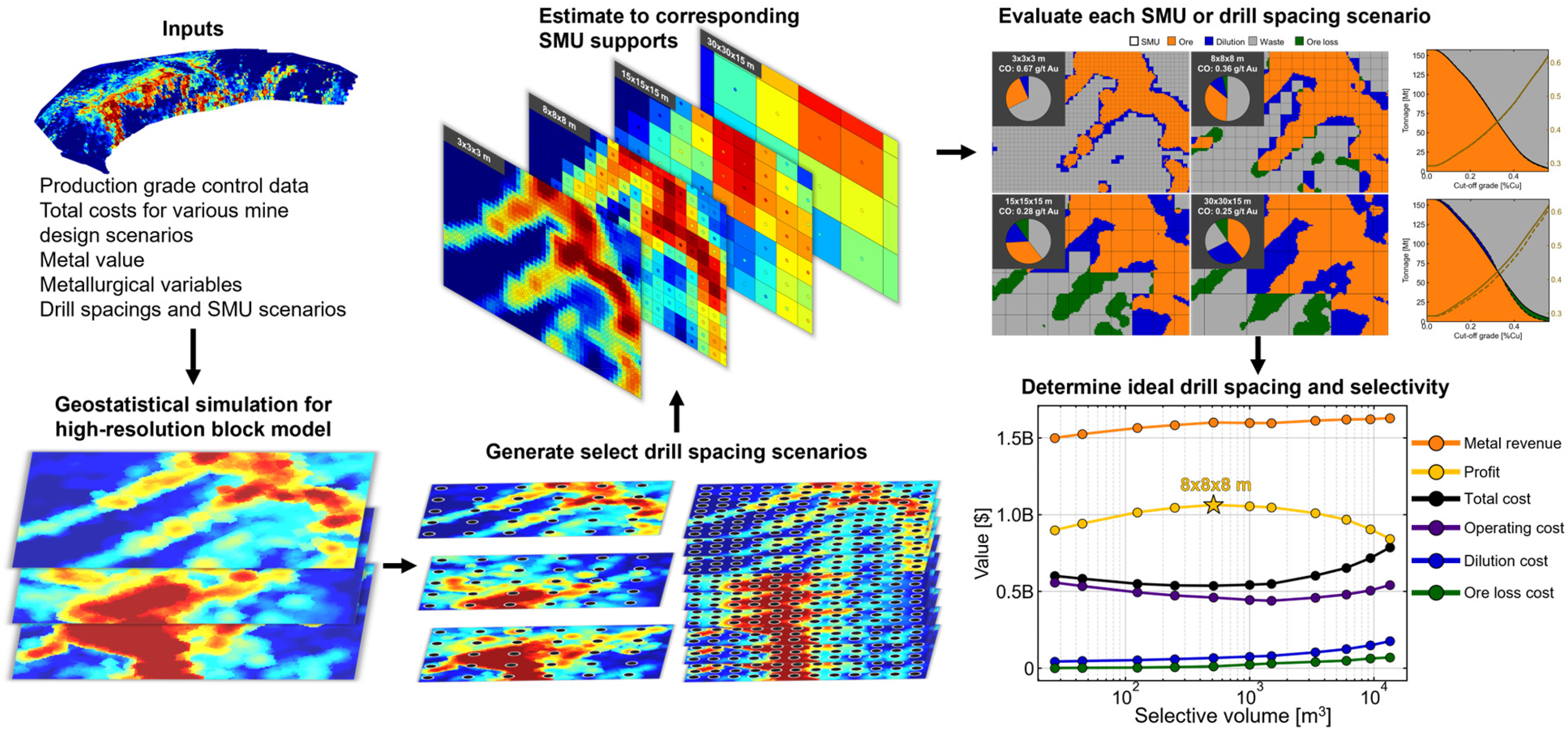
Generalized drillhole spacing and mining selectivity optimization workflow.

Mine design and input parameters for testing

The revenue generated is solely the recovered metal value minus the costs to extract that metal and losses due to dilution plus ore loss. The bare minimum parameters required are the total operating costs, cut-off grade, metal price, density, and metallurgical recovery. The practitioner can input any number of scenarios with a wide range of drillhole spacings and selectivity but the input parameters for a scenario must be defined as accurately as possible for robust results. When optimizing for a mine with an already constrained fleet, the scenarios should be shaped around the mine equipment limitations. For mines with dynamic or flexible fleet options, any scenario which can realistically be achieved could be used. Depending on the mine equipment used, drillhole spacings and mining selectivity can range from 3 × 3 × 3 m (27 m³) to over 30 × 30 × 15 m (13,500 m³). For this study, metallurgical, economic, and operating values following industry trends are used to compare distinctly heterogeneous sites as a case study for testing the workflow and can serve as a baseline if no better information is available.

Simulation of high-resolution block model

Geostatistical simulations have been increasingly used for high-resolution spatial modeling applications as quantifying the variability is a major benefit compared to estimation methods. Here, GSLIB is used to average 25 sequential Gaussian simulations generating the high-resolution block model. The sequential Gaussian simulations are a good starting point and adequate for simple base metal deposits but more complex deposits with significant structural controls like veins, folds, or faults, would benefit by incorporating local varying anisotropy (Boisvert and Deutsch, 2011). Various other simulations methods exist such as multiple point statistics simulation (Strebelle, 2021), sequential indicator simulation (Alabert, 1987), or plurigaussian simulations (Armstrong et al., 2011; Emery, 2007) some of which can be useful for modeling categories before continuous grades. The simulation method which best fits a given deposit should be used for the drillhole spacing and mining selectivity optimization also incorporating the use of domains whenever possible. Even in cases where no formal domains are yet established, if categorical information such as lithology, mineralization, or alteration exist then they can be used with a variety of clustering methods to define domains (Faraj and Ortiz, 2021; MacQueen, 1967).

Regardless of the simulation used, the resolution needs to match the support of the sample which can be done by accounting for what the drilled sample volume would be in equivalent block dimensions. Matching the support can be practically achieved by calculating what the square block length would be based on the drilling diameter using the geometric relationship between the area of a circle and square (Figure 3). The volume of a block can be expressed as:

$${\mathrm{V}}_{\mathrm{B}}={\mathrm{B}}_{\mathrm{l}}{\mathrm{B}}_{\mathrm{w}}{\mathrm{B}}_{\mathrm{h}},$$

(1)

where ${\mathrm{V}}_{\mathrm{B}}$ is the block volume, ${\mathrm{B}}_{\mathrm{l}}$ , ${\mathrm{B}}_{\mathrm{w}}$ , and ${\mathrm{B}}_{\mathrm{h}}$ are the length, width, and height of the block respectively. The cylindrical volume of a drilling sample is:

$${\mathrm{V}}_{\mathrm{C}}=\pi {\mathrm{C}}_{\mathrm{H}}{\left({\displaystyle \frac{{\mathrm{C}}_{\mathrm{d}}}{2}}\right)}^2,$$

(2)

where ${\mathrm{V}}_{\mathrm{C}}$ is the cylindrical volume, ${\mathrm{C}}_{\mathrm{H}}$ is the cylinder height, and ${\mathrm{C}}_{\mathrm{d}}$ is the cylinder diameter. Assuming a square block composited to the same height as the drill sample, the block length can be calculated using the hole diameter:

$$B_l={\displaystyle \frac{C_d}{\sqrt{\pi }}.}$$

(3)

Figure 3.

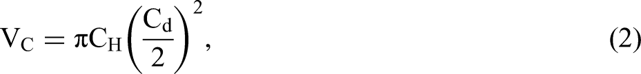
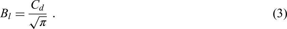
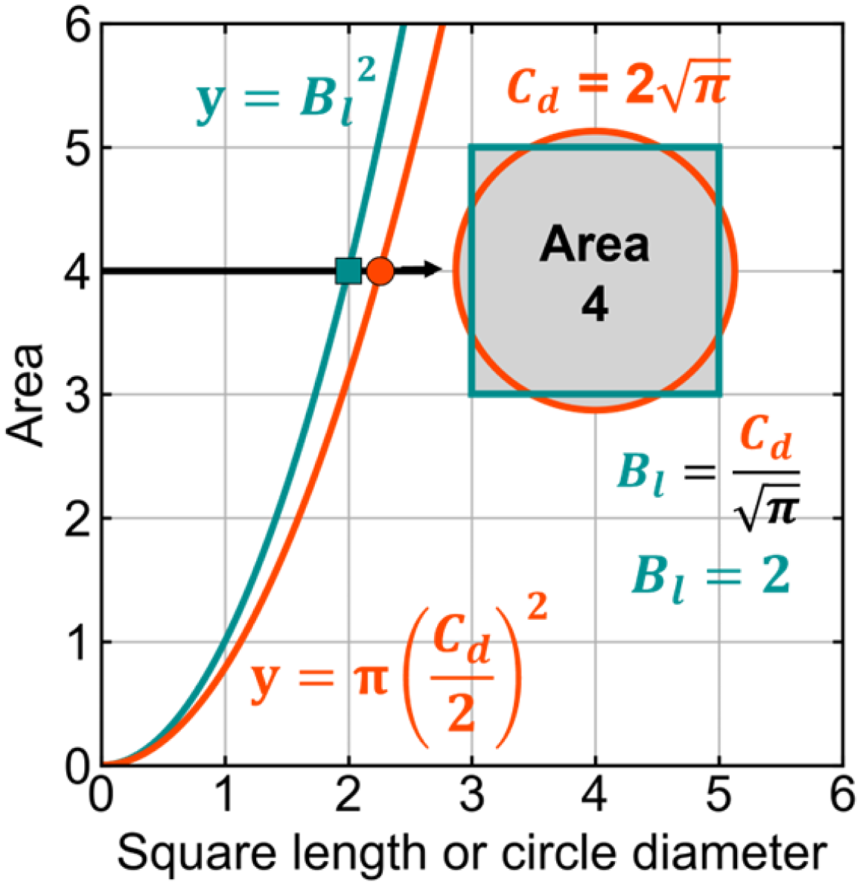
Relationship between area and the square length or circle diameter highlighting how the length of a square multiplied by the square root of pi is the circle diameter of an equivalent area.

Grid cell sizes of 0.125 × 0.125 m which correspond to a drilling diameter of 176 mm are used and composited vertically according to the different bench heights tested. The simulated blocks are aggregated to 1 × 1 × 1 m for comparison purposes with the SMU blocks and allow for computational ease considering the large volumes tested for this study.

Generate drillhole samples and SMU grade estimation

Grids need to be spaced according to each drillhole spacing and SMU scenario defined by the practitioner to draw grades from the simulated block model. A wide range should be set depending on the real conditions of the site so the profit decrease becomes evident in both extremities of drilling too densely or sparsely. The spacings should be carefully considered as Figure 4 shows how the drillhole count scales quadratically with reduced spacing. The simulated block resolution should have been set to reflect the actual drilling volume for samples based on the diameter and can be later aggregated to match the SMU support for comparison purposes. While testing a wide range of drillhole spacings and selectivity should be pursued, changes will have a significant impact especially if the drillholes are for both grade control and production blasting as there will be constraints on balancing the hole diameter, bench height, burden, and spacing.

Figure 4.

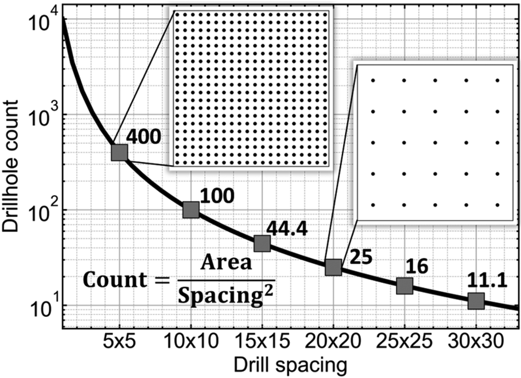
Quadratic relationship between the area, drill spacing, and drillhole count for an area of 100 × 100.

Similar to the type of simulation used to generate the high-resolution model, the SMU block grades can be estimated with any method. Ordinary kriging is used for all the scenarios in this case study and is also traditionally used in the industry to estimate grades (Krige, 1951; Matheron, 1963). Other types of estimation may be more appropriate depending on the deposit such as different types of kriging like simple kriging or universal kriging where appropriate (Daya and Bejari, 2015; Zimmerman et al., 1999), non-parametric methods (Journel, 1983), or adaptive spatial inverse distance weighted methods for rare cases where the data cannot be modeled well with typical variogram functions (Lu and Wong, 2008).

Evaluating the drillhole spacing and mining selectivity scenarios

The estimated SMU blocks for each scenario are compared to the simulated truth block model. While an estimated grade may not accurately match the true grade, the important requirement is how the material is classified based on a cutoff grade or material classification scheme. There will be cases where the material type is aligned as either ore or waste and there will be cases where ore is estimated when it is truly waste causing dilution or waste estimated where there is truly ore causing ore loss. The dilution is calculated with:

$$\mathrm{Dilution}(\text{\%})=100{\displaystyle \frac{{\mathrm{T}}_{\mathrm{D}}}{{\mathrm{T}}_{\mathrm{D}}+{\mathrm{T}}_{\mathrm{ore}}},}$$

(4)

where ${\mathrm{T}}_{\mathrm{ore}}$ is the tonnes of ore, ${\mathrm{T}}_{\mathrm{D}}$ is the tonnes of dilution. The ore loss is calculated with:

$$\mathrm{Ore}\mathrm{loss}(\text{\%})=100{\displaystyle \frac{{\mathrm{T}}_{\mathrm{OL}}}{{\mathrm{T}}_{\mathrm{OL}}+{\mathrm{T}}_{\mathrm{waste}}},}$$

(5)

where ${\mathrm{T}}_{\mathrm{OL}}$ is the tonnes of ore loss, and ${\mathrm{T}}_{\mathrm{waste}}$ is the tonnes of waste. The total dilution and ore loss plus their average grade relative to the cutoff grade becomes relevant for calculating the profit which is the metric driving the drillhole spacing and mining selectivity optimization. The profit is calculated using:

$$\mathrm{Profit}={\mathrm{T}}_{\mathrm{ore}}{\mathrm{Z}}_{\mathrm{ore}}{\mathrm{RS}}_{\mathrm{p}}-{\mathrm{T}}_{\mathrm{ore}}{\mathrm{C}}_{\mathrm{t}}-{\mathrm{T}}_{\mathrm{D}}({\mathrm{Z}}_{\mathrm{CO}}-{\mathrm{Z}}_{\mathrm{D}}){\mathrm{RS}}_{\mathrm{p}}-{\mathrm{T}}_{\mathrm{OL}}({\mathrm{Z}}_{\mathrm{OL}}-{\mathrm{Z}}_{\mathrm{CO}}){\mathrm{RS}}_{\mathrm{p}},$$

(6)

where ${\mathrm{Z}}_{\mathrm{ore}}$ is the average ore grade, $\mathrm{R}$ is the recovery, ${\mathrm{S}}_{\mathrm{p}}$ is the selling price, ${\mathrm{C}}_{\mathrm{t}}$ is the total cost per tonne of ore, ${\mathrm{Z}}_{\mathrm{CO}}$ is the cutoff grade, ${\mathrm{Z}}_{\mathrm{D}}$ is the average dilution grade, and ${\mathrm{Z}}_{\mathrm{OL}}$ is the average ore loss grade. This simplistic formulation for profit requires the cutoff grade to be calculated as a function of the total cost per tonne of ore:

$${\mathrm{Z}}_{\mathrm{CO}}={\displaystyle \frac{{\mathrm{C}}_{\mathrm{t}}}{{\mathrm{RS}}_{\mathrm{p}}}.}$$

(7)

The profit calculation is simplified for this case study to accommodate the wide range of scenarios for the three mines in this controlled application but should be adapted for specific cases. When considering a specific site, the location, geology for metallurgical parameters such as hardness and recovery, capital expenditures, and local operating costs can all be estimated accurately making the profit calculation appropriately more complex and accurate.

Application on distinctly heterogeneous open pit mines

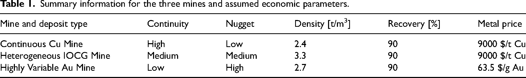
The drillhole spacing and mining selectivity workflow is applied on one year of real production data from three increasingly heterogeneous mines: a continuous Cu porphyry mine, a heterogeneous iron-oxide copper gold (IOCG) mine, and a highly variable vein hosted Au mine. Summary information of each mine is summarized in Table 1 with the assumed economic parameters for the study. The dataset from each mine spans hundreds of meters in each direction and Figure 5 shows how each has a clear difference in the grade distribution and continuity. The three mines capture a wide range in heterogeneity to compare how the optimal drillhole spacing and mining selectivity varies.

Figure 5.

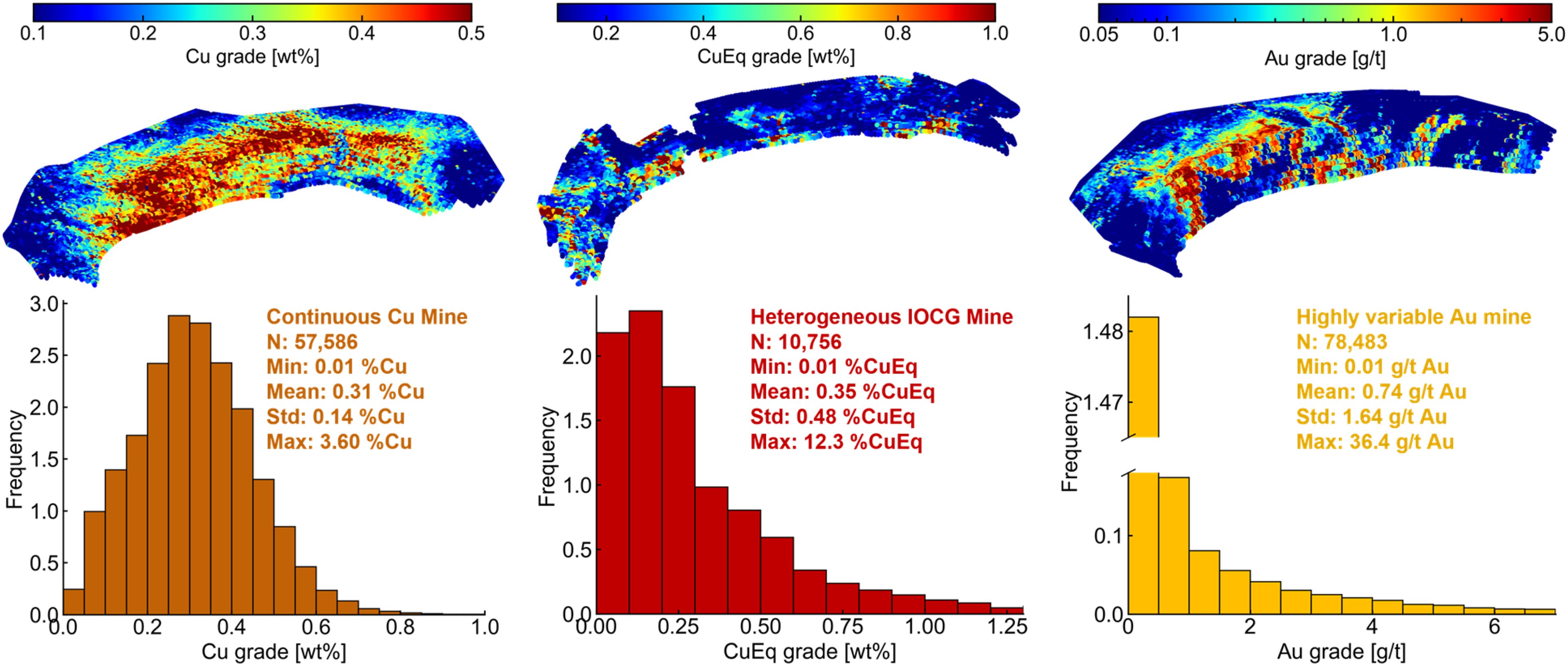
Spatial plots and histograms with descriptive statistics for the production data for the continuous cu mine, heterogeneous IOCG mine, and highly variable Au mine.

Table 1.

Summary information for the three mines and assumed economic parameters.

Mine and deposit type	Continuity	Nugget	Density [t/m3]	Recovery [%]	Metal price
Continuous Cu Mine	High	Low	2.4	90	9000 $/t Cu
Heterogeneous IOCG Mine	Medium	Medium	3.3	90	9000 $/t Cu
Highly Variable Au Mine	Low	High	2.7	90	63.5 $/g Au

Testing scenarios and cost assumptions

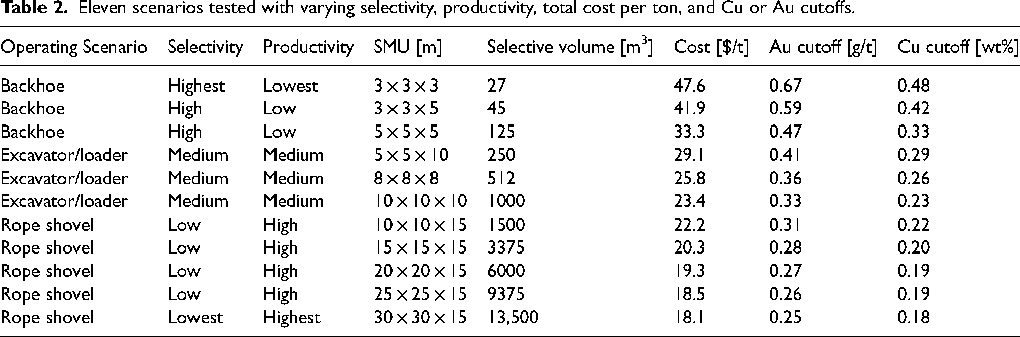
Eleven drillhole spacing and SMU size scenarios are tested covering a wide range of selectivity for each of the three mines. Table 2 describes the operating scenario, SMU dimensions, costs, and cutoffs applied. Data from Crowson, (2003) relates the mine cost to its scale and is used to inform the costs used for each scenario studied (Figure 6). The wide range of drilling spacing and mining selectivity is required in this case as data from significantly distinct deposits is used where large differences are expected for the tested scenarios. In a more constrained application, more scenarios can be used in a smaller range of drillhole spacing and mining selectivity to define the optimal result in greater detail.

Figure 6.

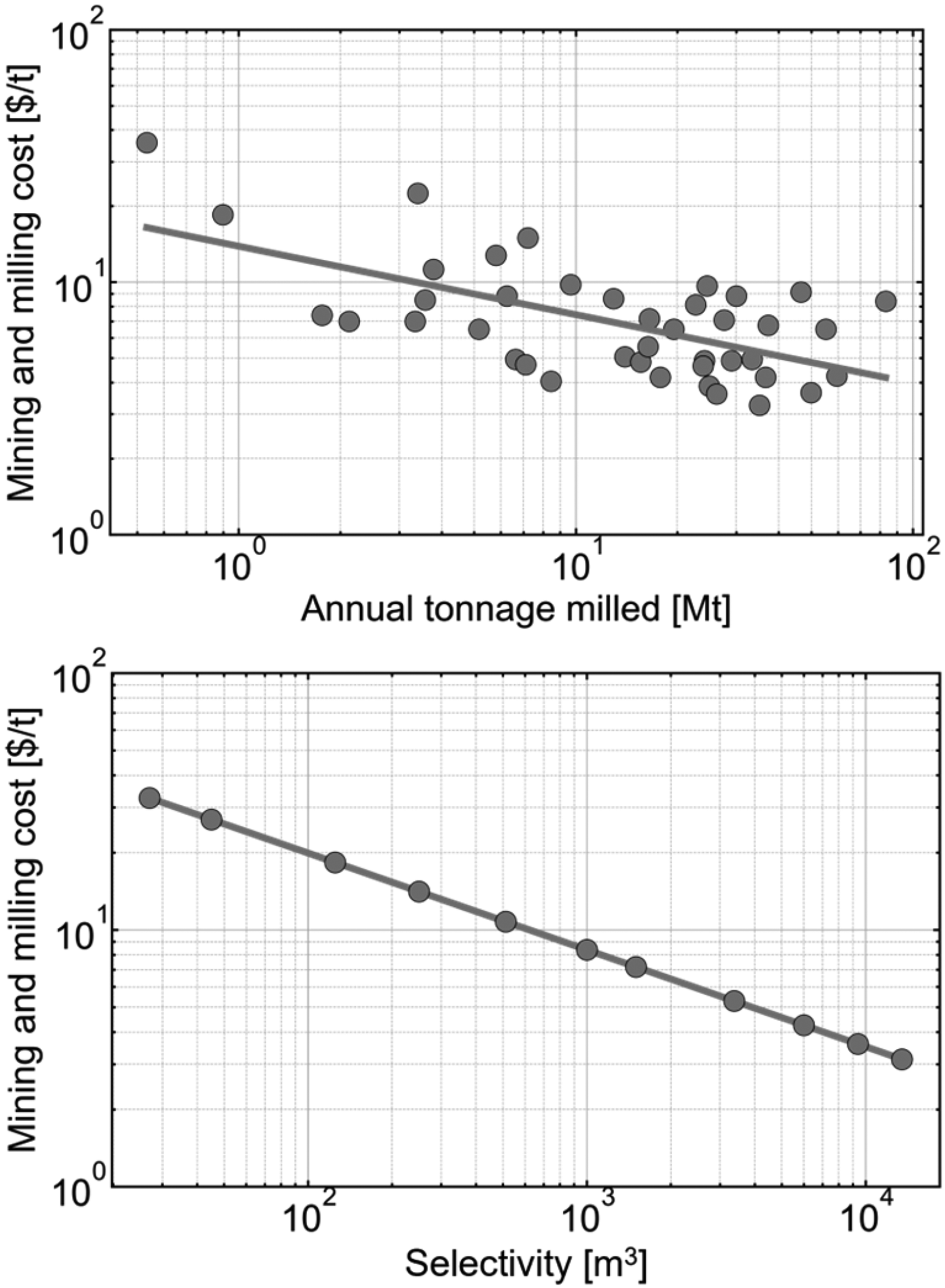
Decreasing cost relationship with increasing annual tonnage milled (data from Crowson, 2003) trend used to assume the cost selectivity relationship for this study.

Table 2.

Eleven scenarios tested with varying selectivity, productivity, total cost per ton, and Cu or Au cutoffs.

Operating Scenario	Selectivity	Productivity	SMU [m]	Selective volume [m3]	Cost [$/t]	Au cutoff [g/t]	Cu cutoff [wt%]
Backhoe	Highest	Lowest	3 × 3 × 3	27	47.6	0.67	0.48
Backhoe	High	Low	3 × 3 × 5	45	41.9	0.59	0.42
Backhoe	High	Low	5 × 5 × 5	125	33.3	0.47	0.33
Excavator/loader	Medium	Medium	5 × 5 × 10	250	29.1	0.41	0.29
Excavator/loader	Medium	Medium	8 × 8 × 8	512	25.8	0.36	0.26
Excavator/loader	Medium	Medium	10 × 10 × 10	1000	23.4	0.33	0.23
Rope shovel	Low	High	10 × 10 × 15	1500	22.2	0.31	0.22
Rope shovel	Low	High	15 × 15 × 15	3375	20.3	0.28	0.20
Rope shovel	Low	High	20 × 20 × 15	6000	19.3	0.27	0.19
Rope shovel	Low	High	25 × 25 × 15	9375	18.5	0.26	0.19
Rope shovel	Lowest	Highest	30 × 30 × 15	13,500	18.1	0.25	0.18

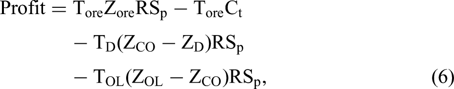
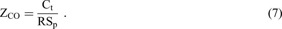
The total cost per tonne is calculated using:

$${\mathrm{C}}_{\mathrm{t}}=3.1347\cdot {{\mathrm{S}}_{\mathrm{n}}}^{-0.377}+15,$$

(8)

where ${\mathrm{S}}_{\mathrm{n}}$ is the 27 to 13,500 m³ normalized selectivity based on the data from Crowson (2003) and 15 $/t is added to reflect other costs ignored such as metal selling cost, smelter penalties, waste mining, and general and administrative expenses for the purpose of fairly comparing the data from three distinct mines. The coarse assumptions are made to compare and assess the three distinct mines under controlled settings to better study how the underlying heterogeneity impacts the optimal drillhole spacing and mining selectivity.

Data resolution impact on ore loss and dilution

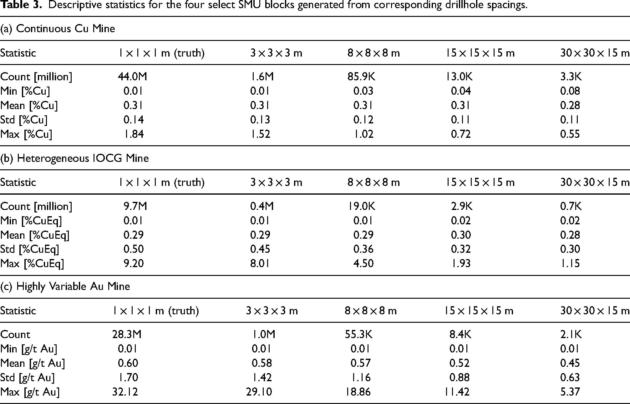
The sequential Gaussian simulations returned 44.0, 9.7, and 28.3 million 1 × 1 × 1 m blocks for the continuous Cu mine, heterogeneous IOCG mine, and highly variable Au mine respectively. As expected, the average grade of the tighter drilling spacing and correspondingly more selective SMU blocks better matched the simulated true 1 × 1 × 1 m block grades (Table 3). For the copper mines the average grade of all the scenarios was within 10% while for the more variable Au mine the average grade of the highly selective 3 × 3 × 3 m scenario achieved similar accuracy within 5% but for the least selective 30 × 30 × 15 m scenario the average grade was off by −25% likely as many of the veins and mineralized structures are missed by the sparser drillhole spacing. Also, the variance reduction factor due to the change of support from the simulated 1 × 1 × 1 m block grades to the least selective 30 × 30 × 15 m scenario increased from 38%, to 64%, and up to 88% for the continuous Cu mine, heterogeneous IOCG mine, and highly variable Au mine expectedly as the trend matches the increasing nugget effect in the three mines.

Table 3.

Descriptive statistics for the four select SMU blocks generated from corresponding drillhole spacings.

(a) Continuous Cu Mine
Statistic	1 × 1 × 1 m (truth)	3 × 3 × 3 m	8 × 8 × 8 m	15 × 15 × 15 m	30 × 30 × 15 m
Count [million]	44.0M	1.6M	85.9K	13.0K	3.3K
Min [%Cu]	0.01	0.01	0.03	0.04	0.08
Mean [%Cu]	0.31	0.31	0.31	0.31	0.28
Std [%Cu]	0.14	0.13	0.12	0.11	0.11
Max [%Cu]	1.84	1.52	1.02	0.72	0.55

(b) Heterogeneous IOCG Mine
Statistic	1 × 1 × 1 m (truth)	3 × 3 × 3 m	8 × 8 × 8 m	15 × 15 × 15 m	30 × 30 × 15 m
Count [million]	9.7M	0.4M	19.0K	2.9K	0.7K
Min [%CuEq]	0.01	0.01	0.01	0.02	0.02
Mean [%CuEq]	0.29	0.29	0.29	0.30	0.28
Std [%CuEq]	0.50	0.45	0.36	0.32	0.30
Max [%CuEq]	9.20	8.01	4.50	1.93	1.15

(c) Highly Variable Au Mine
Statistic	1 × 1 × 1 m (truth)	3 × 3 × 3 m	8 × 8 × 8 m	15 × 15 × 15 m	30 × 30 × 15 m
Count	28.3M	1.0M	55.3K	8.4K	2.1K
Min [g/t Au]	0.01	0.01	0.01	0.01	0.01
Mean [g/t Au]	0.60	0.58	0.57	0.52	0.45
Std [g/t Au]	1.70	1.42	1.16	0.88	0.63
Max [g/t Au]	32.12	29.10	18.86	11.42	5.37

The grade maps to the left of Figure 7 show the distinct continuity of grades in each of the mines and loss in resolution plus smoothing especially for the less selective, widely spaced drillhole scenarios. The Au mine in Figure 7(a) with the most selective 3 × 3 × 3 m SMU scenario demonstrates how the Au grades vary by two orders of magnitude from 0.05 g/t Au to 5 g/t Au in the span of a few meters while the continuous Cu mine grades in Figure 7(c) vary at most by a factor of 3 from 0.1%Cu to 0.3%Cu over more than 10 m. The heterogeneous IOCG mine demonstrates both continuous zones and areas of high variability throughout the grade map in Figure 7(b).

Figure 7.

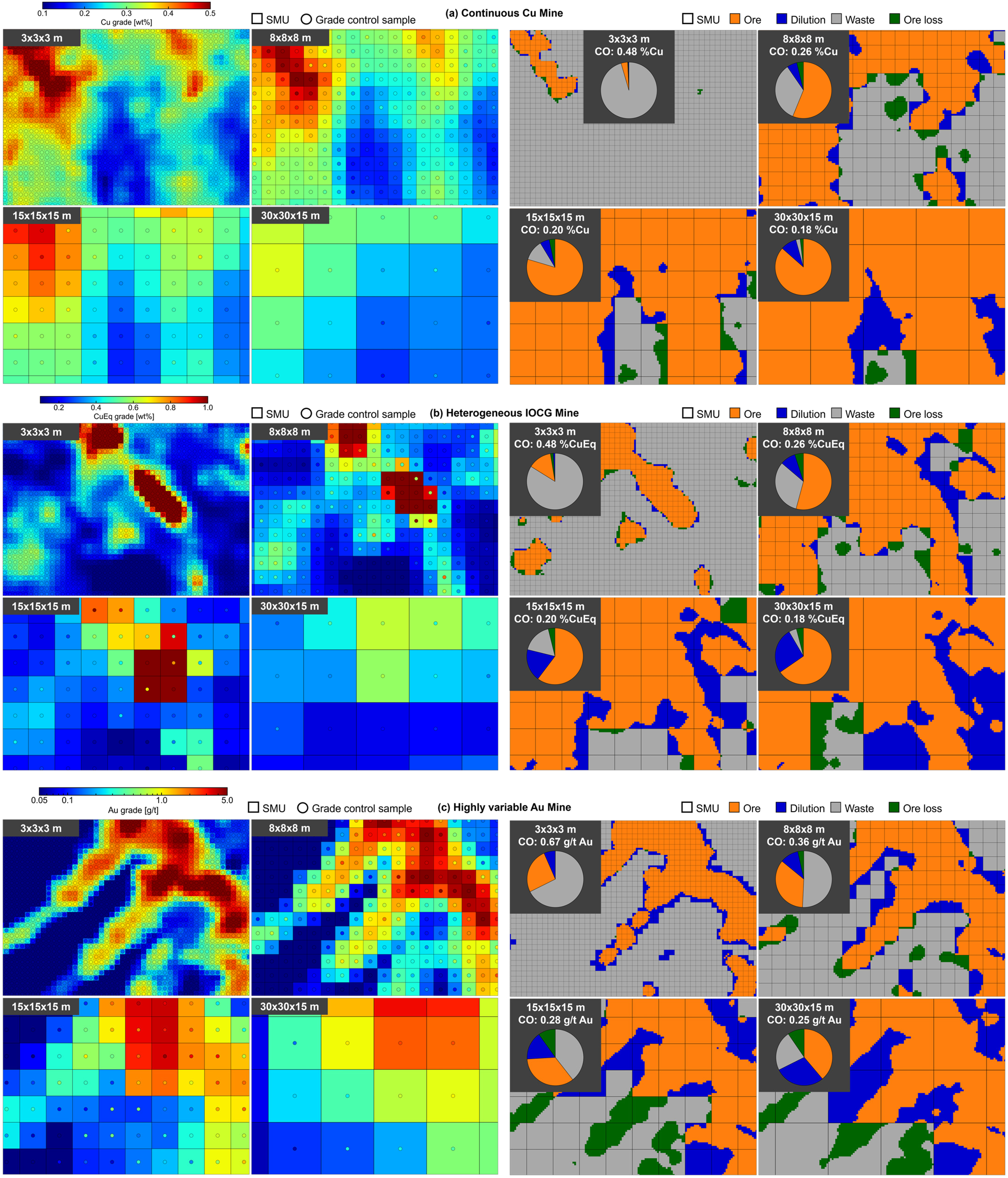
Areas with ore/waste contacts demonstrating SMU grades with grade control samples to the left and material classification maps with a pie chart showing the percent of each material to the right at the select SMU scenarios for the (a) continuous cu mine, (b) heterogeneous IOCG mine, and (c) highly variable Au mine.

The material classification maps to the right of Figure 7 show how the ore loss and dilution increase as the selectivity and drillhole spacing widens. In the continuous Cu mine map, the percentage of ore loss plus dilution blocks never exceed 20% of the total material classification in the map even in the least selective 30 × 30 × 15 m scenario suggesting the cost savings using wider drillhole spacings may outweigh the lost value due to ore loss and dilution (Figure 7(a)). The percentage of ore loss plus dilution blocks in the case of the highly variable Au mine, on the other hand, shows nearly 50% of the material classified as ore loss or dilution suggesting that the added cost of the tighter drillhole spacing in one of the more selective scenarios will be worthwhile (Figure 7(c)). Similarly to the grade maps, the optimal drillhole spacing and mining selectivity for the heterogeneous IOCG mine likely falls somewhere between the two but visually is hard to determine and needs to be quantified (Figure 7(b)).

For all three mines the strip ratio decreases as the drillhole spacing and SMU size widens due, by design, to the cutoff change triggered by the higher costs per ton. The change in relative amounts of ore and waste is especially clear for the continuous Cu mine scenarios the ore/waste split increases nearly ten times from 9% ore and 91% waste to 83% ore and 17% waste since the distribution of grades for the high tonnage low grade deposit is most concentrated around the cutoff range (Figure 8(a)). For the highly variable Au mine scenarios the split only doubles from 13% ore and 87% waste to only 26% ore and 74% waste due to the high amount of waste present and low tonnage but high grade ore (Figure 8(c)). The ore/waste split for the heterogeneous IOCG mine scenarios increases by a factor of three from 17% ore and 81% waste to 53% ore and 47% waste (Figure 8(b)). For all mines the dilution plus ore loss increases for the less selective scenarios and the relative grade difference between the dilution or ore loss respective to the cutoff increases for the more variable mines (Figure 8).

Figure 8.

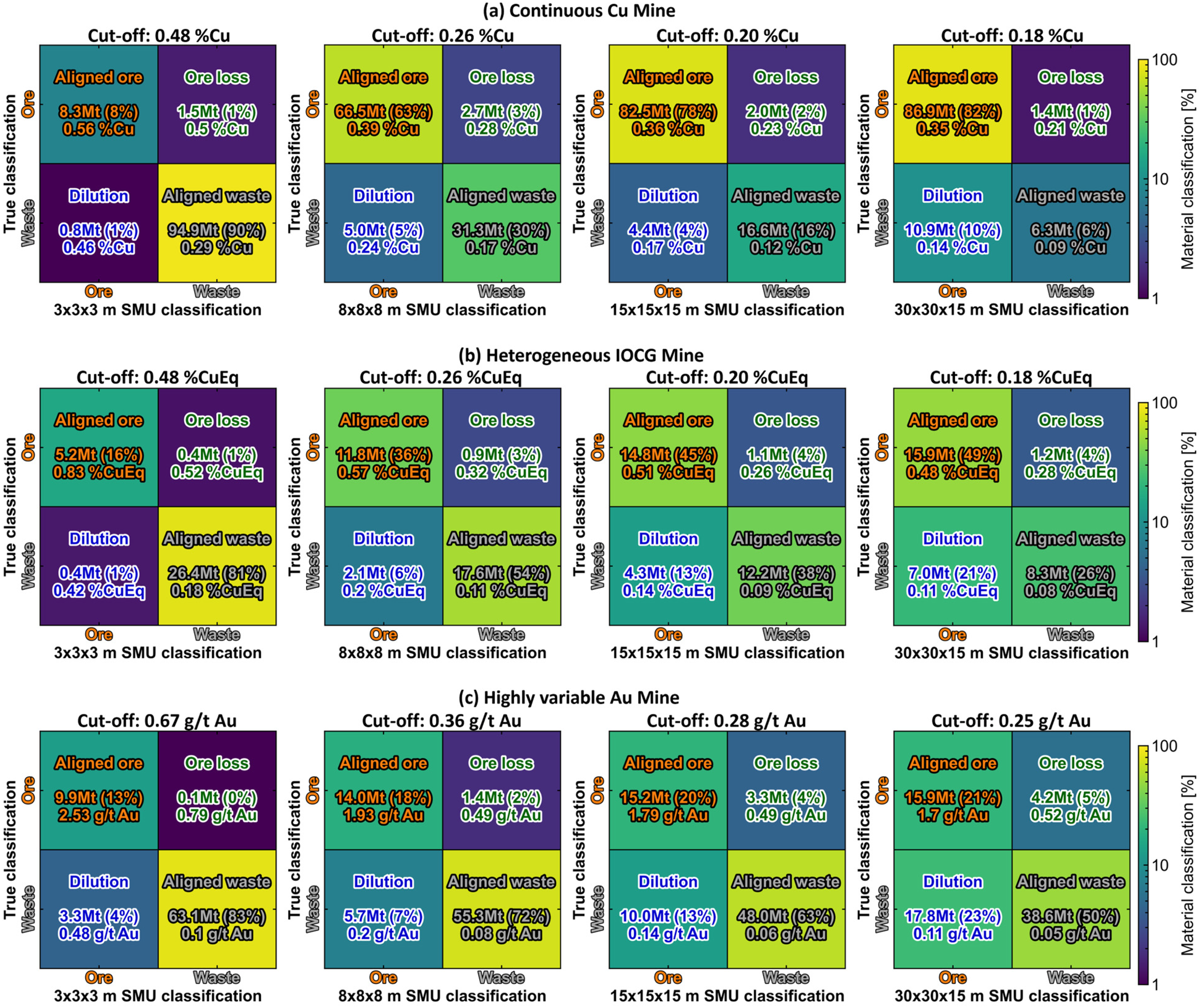
Confusion matrices showing the aligned ore, ore loss, dilution, and aligned waste classifications, tonnages, and grades of the select SMU scenarios for the (a) continuous Cu mine, (b) heterogeneous IOCG mine, and (c) highly variable Au mine. Note the numbers may not add up due to rounding.

Across the entire drillhole spacings and SMU scenarios the percentage of dilution plus ore loss for the highly variable Au mine only appears to be about three times higher than the continuous Cu mine and two times higher than the heterogeneous IOCG mine (Figure 9). While percentages of dilution plus ore loss are do not seem as different in the three mines, the copper mines have much more opportunity for dilution and ore loss to take place because the larger proportion of the distribution is within the cutoff range. The dilution and ore loss percentages do not consider the degree of grade difference from the cutoff which is captured in profit calculation and Figure 9 shows how the impact of dilution plus ore loss is more than five times for the highly variable Au mine compared to the continuous Cu mine depending on the scenario. While the highly variable Au mine does not have the same amount of transitional material, the potential dilution of barren waste and loss of high grade ore have a much greater impact than dilution or ore loss with grades right around the cutoff.

Figure 9.

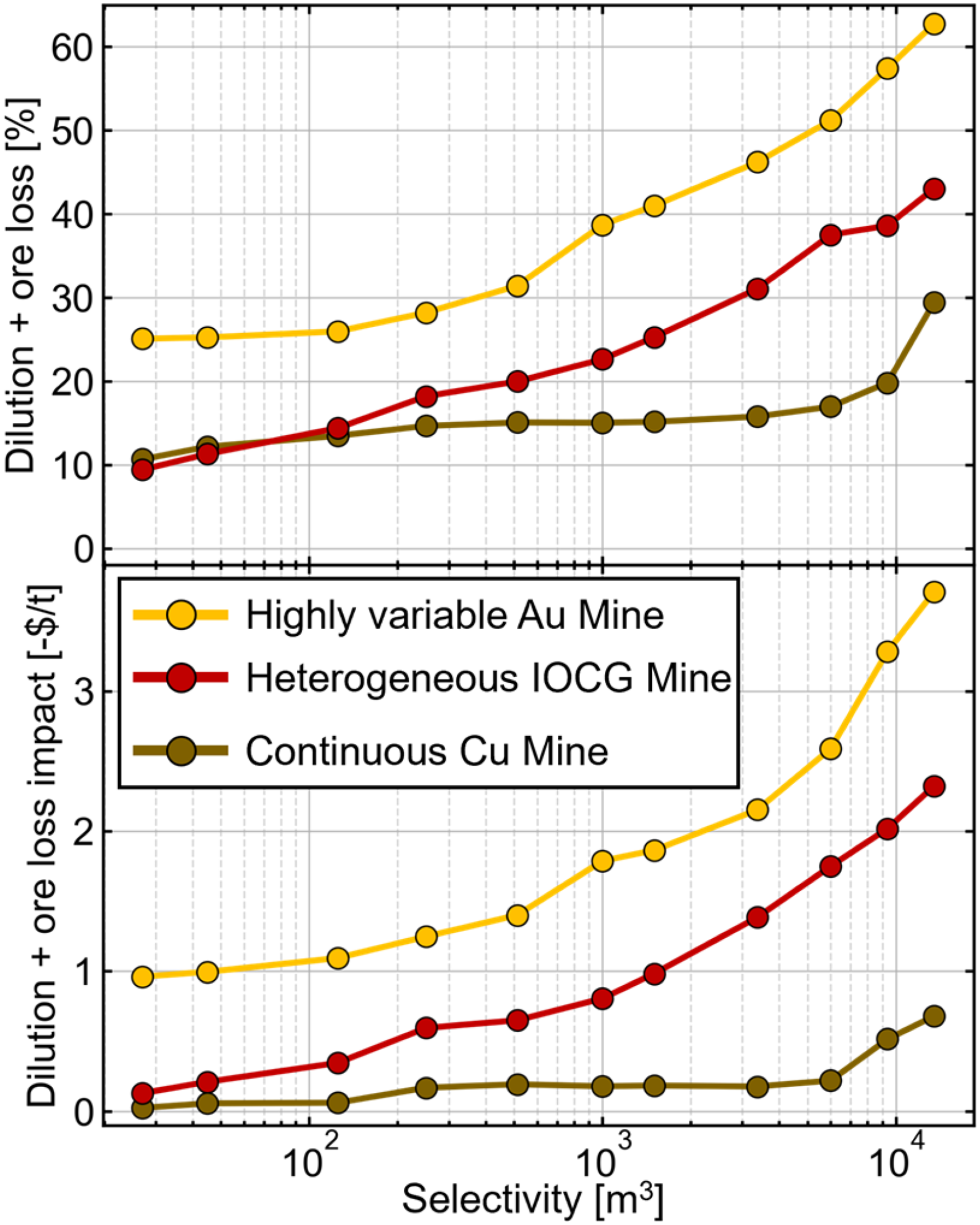
Dilution plus ore loss percentages and profit loss expressed in -$/t demonstrating how the economic impact scales with the deposit's variability and is not as evident with just the percent dilution plus ore loss.

Optimal drillhole spacing and mining selectivity

Evaluating the eleven drillhole spacing and mining selectivity scenarios returned a different optimum point for each mine. For the continuous Cu mine the optimal drillhole spacing and mining selectivity is 25 × 25 × 15 m (9375 m³) while the heterogeneous IOCG mine resulted in 15 × 15 × 15 m (3375 m³) and the highly variable Au mine with the most selective 8 × 8 × 8 m (512 m³) result (Figure 10). The normalized profit curves for the copper mines in Figure 10 demonstrate how tighter drillhole spacing and more selective mining resulted in significantly lower value compared to the sparser drilling and less selective case until reaching the least selective scenarios. The opposite is true for the Au mine where the tighter drillhole spacing and more selective mining method scenario achieved a higher profit until a certain point where it started to reduce below the 8 × 8 × 8 m scenario (512 m³).

Figure 10.

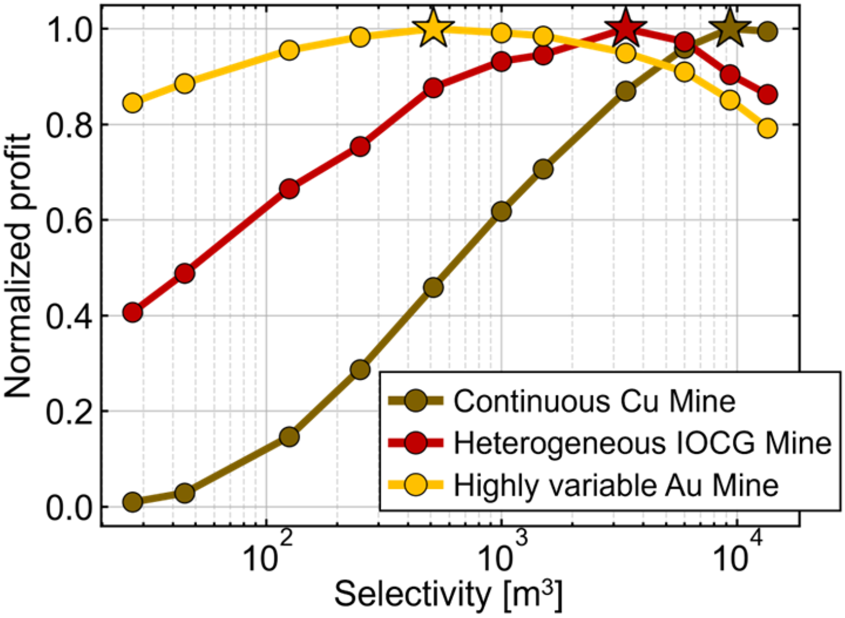
Normalized profit and revenue minus cost breakdown showing the optimal drillhole spacing and mining selectivity for each mine.

Using a large number of scenarios at small intervals from each other is important to determine the optimal point. When considering the nearest neighboring scenarios from the optimum, the profit for the continuous Cu, heterogeneous IOCG, and highly variable Au mines go down by 1%, 8%, and 3% respectively. When considering the entire range of scenarios tested, the continuous Cu mine drops the most dramatically to about 1% demonstrating how investing in expensive selective mining is not effective for a homogeneous high tonnage low grade deposit where most of the material is all ore (Figure 11(a)). The heterogeneous IOCG mine has more barren waste scattered throughout the orebody and the profit in all scenarios tested drops to 41% for the most selective 3 × 3 × 3 m scenario (27 m³) and drops to 84% in the least selective 30 × 30 × 15 m scenario (13,500 m³). In the case of the Au mine the profit is lowest achieving 78% of the optimal profit at the widest drillhole spacing and least selective 30 × 30 × 15 m (13,500 m³) scenario but is not much different than the 83% achieved at the most selective scenario (Figure 10). The highly variable Au mine does not fluctuate as much as the copper mines likely because both areas of extreme heterogeneity and homogeneity exist (Figure 11(c)). The grade tonnage curves in Figure 11 show how the tonnage varies across the cutoff range and the increasing difference between the less selective scenarios to the 1 × 1 × 1 m truth especially in the case of the more variable deposits.

Figure 11.

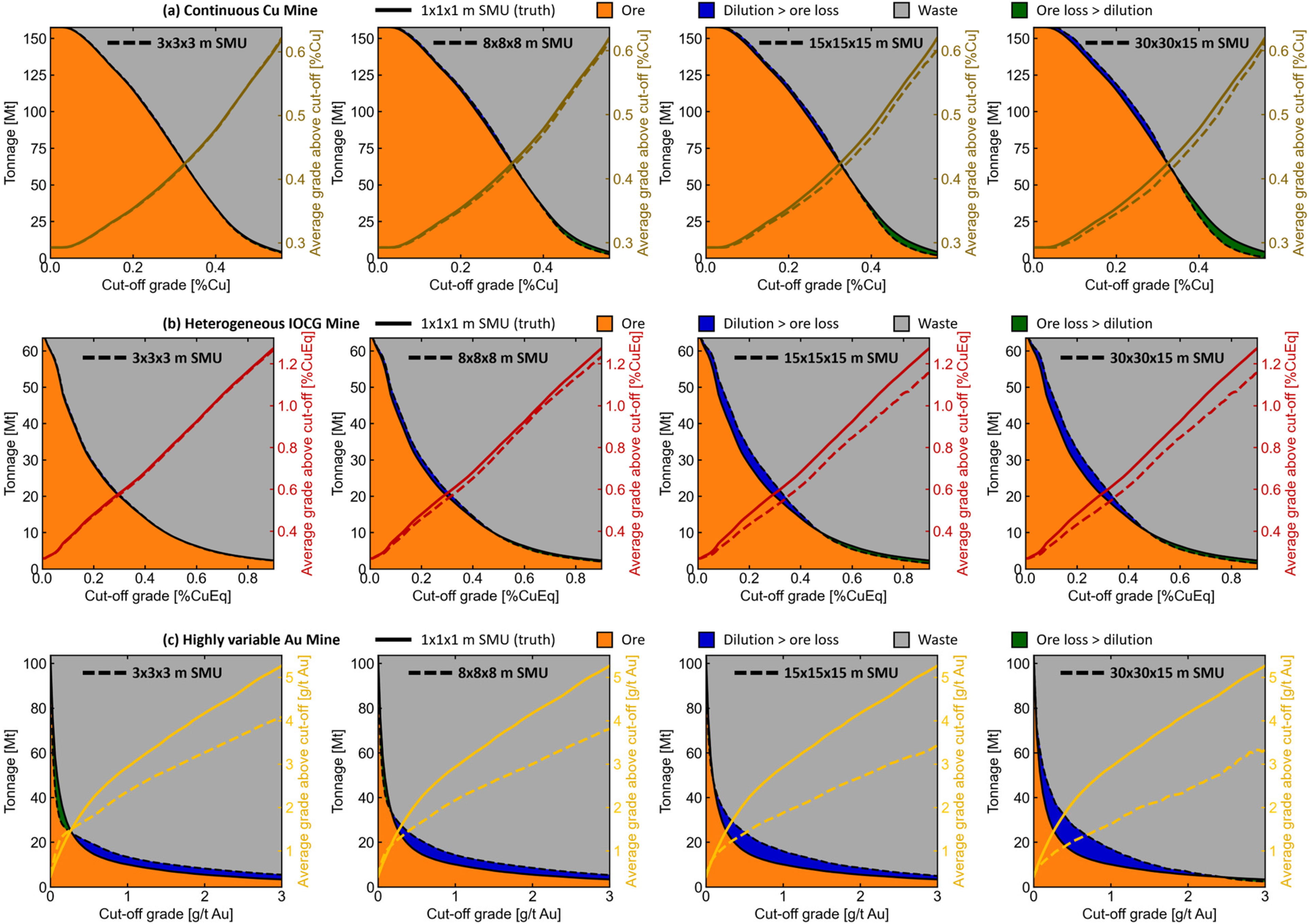
Grade tonnage curves the select resolutions for the (a) continuous Cu mine, (b) heterogeneous IOCG mine, and (c) highly variable Au mine.

The cost and revenue curves throughout the eleven drillhole spacing and mining selectivity scenarios in Figure 12 varied significantly for the three mines. As the drillhole spacing widens and selectivity decreases, the total metal revenue increases with the profit until it eventually starts losing value due to the incremental dilution and ore loss cost. For more homogeneous copper deposits, opting for less selective but cheaper mining will typically be the better decision while the opposite is true for more heterogeneous deposits such as the highly variable Au mine. An important artifact to consider is the changing breakeven cutoff reflecting the increasing operating cost for the more selective scenarios. The changing cutoff had the biggest impact for the continuous Cu mine since most of the grades are within the cutoff range while for the Au mine it had a smaller impact since most of the grades are barren waste or high grade ore without much medium grade around the cutoff range. The profit loss due to dilution plus ore loss increases for the more variable mines and as the selectivity decreases which can be more easily observed in Figure 12 by comparing the total cost curve to the operating cost curve as their difference would be the dilution plus ore loss cost.

Figure 12.

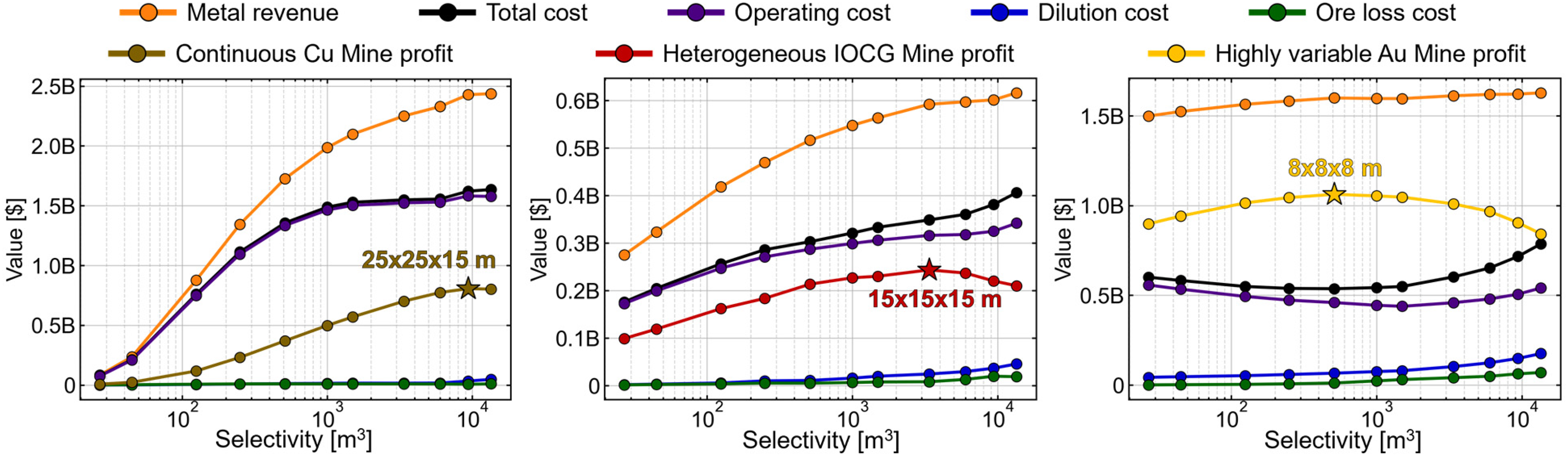
Metal revenue and cost breakdown showing the optimal drillhole spacing and mining selectivity scenario for each mine.

Workflow potential and limitations

The drillhole spacing and mining selectivity optimization workflow can be used for other applications such as defining areas of distinct enough heterogeneity where decisions can be made to increase ore control effort or determine the potential of investing in ore sorting equipment. Given the large number of inputs and steps to achieve a result, careful consideration is required so all the variables are defined as accurately as possible to generate robust results. The following subsections discuss the workflow potential along with its limitations and recommendations to ensure meaningful results are achieved and the modeling sensitivities understood.

Determining heterogeneity for ideal mining selectivity and ore sorting potential

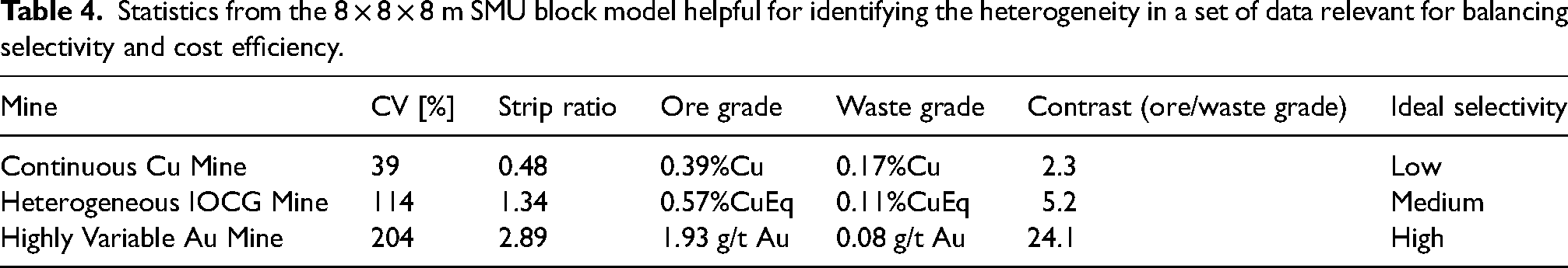
Practitioners can use different mining statistics such as the coefficient of variation (CV), strip ratio, and ore to waste grade contrast to determine where different domains of a single mine or mine with multiple pits will fall under the heterogeneity spectrum. Table 4 compares these statistics for the three mines showing intuitive trends for when the additional effort of mining more selectively is worth the cost. The CV provides an idea of the variability in the grades while the strip ratio reveals the relative proportions of ore and waste and importantly the ore to waste grade contrast is an indicator of the dilution plus ore loss cost magnitude. While increasing CV and contrast will likely scale with increasing selectivity, either extremity in strip ratio of less than 0.5 or greater than 10 will detract from more selective mining.

Table 4.

Statistics from the 8 × 8 × 8 m SMU block model helpful for identifying the heterogeneity in a set of data relevant for balancing selectivity and cost efficiency.

Mine	CV [%]	Strip ratio	Ore grade	Waste grade	Contrast (ore/waste grade)	Ideal selectivity
Continuous Cu Mine	39	0.48	0.39%Cu	0.17%Cu	2.3	Low
Heterogeneous IOCG Mine	114	1.34	0.57%CuEq	0.11%CuEq	5.2	Medium
Highly Variable Au Mine	204	2.89	1.93 g/t Au	0.08 g/t Au	24.1	High

These parameters can be used to evaluate different volumes of a mine as the grade control scenario may have a different optimum if there exist areas of distinct heterogeneity. While the main use case is for improving short range grade control, the tool could be used for planning future pushbacks assuming data exists from a previous but similar pushback which can be used as an analogue. Even data from similar deposits could be used to inform the mine design and equipment used.

The workflow can also be used to quantify the potential profit of investing in ore sorting equipment which allows the mine to sort at a higher selectivity without the added cost of more selective mining equipment like switching to flitch mining with backhoes. To calculate what the potential profit would be with ore sorting equipment, the dilution and ore loss cost can simply be switched with the cost from the more selective scenario as shown in Figure 13. Bulk ore sorting systems such as bucket mounted X-ray fluorescence sensors exist to divert trucks at the mine face (Faraj et al., 2022) and belt-based ore sorting systems also exist leveraging prompt gamma neutron activation analysis (PGNAA) technology. Considerations will be required that the ore sorting system is amenable to the orebody. For example, XRF on a shovel may be a better choice to recover ore from mined waste at the mine face but can’t measure Au which a PGNAA belt sorter can measure and potentially create high value in cases such as the highly variable Au mine where dilution is much greater than ore loss (Kurtha and Balzanb, 2022).

Figure 13.

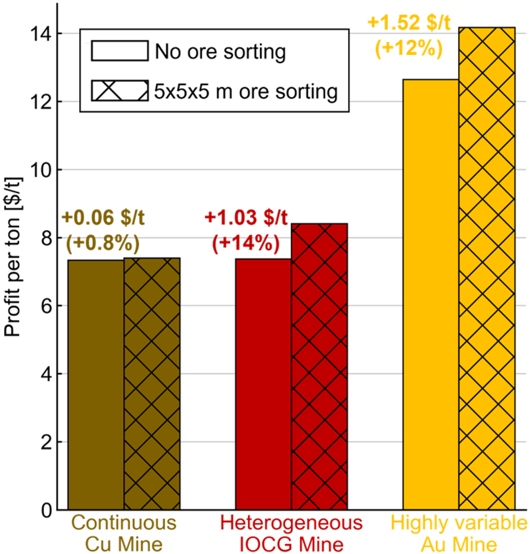
Profit per tonne increased by reducing the dilution and ore loss of the 20 × 20 × 15 m scenario assuming the ore can be sorted at a selectivity of 5 × 5 × 5 m at the same cost.

Sensitivity to value driving decision variables

The drillhole spacing and mining selectivity optimization workflow is dependent and sensitive to the various inputs for calculating the profit. Broad operating cost and cutoff assumptions were made to consistently compare different deposits but any detailed cost estimation for two different sites will vary significantly. The recovery and metal price also have big implications since they affect both the metal revenue and dilution plus ore loss cost. Assigning recovery, metal price, and operating costs will each affect and drive the optimized result and could have compounding effects if biased in the same way.

As the operating cost for each scenario, metal price, and recovery go down the workflow will bias towards more selective cases while when the same inputs increase the optimums will trend towards less selective cases (Figure 14). The proposed method was shown to be adequate for the controlled comparison of multiple deposits but to optimize the drillhole spacing and mining selectivity of a single site, every input parameter needs to be carefully considered and the scenarios should be constrained for what is feasible based on the existing mine equipment. Using the drillhole spacing and mining selectivity scenario range here from of 3 × 3 × 3 m (27 m³) to 30 × 30 × 15 m (13,500 m³) is useful to compare volumes spanning both extremes of natural variability. When the deposit is known to be a homogeneous Cu porphyry or heterogeneous vein hosted Au mine the scenario range should be narrowed down allowing for finer steps to better approximate the optimal result.

Figure 14.

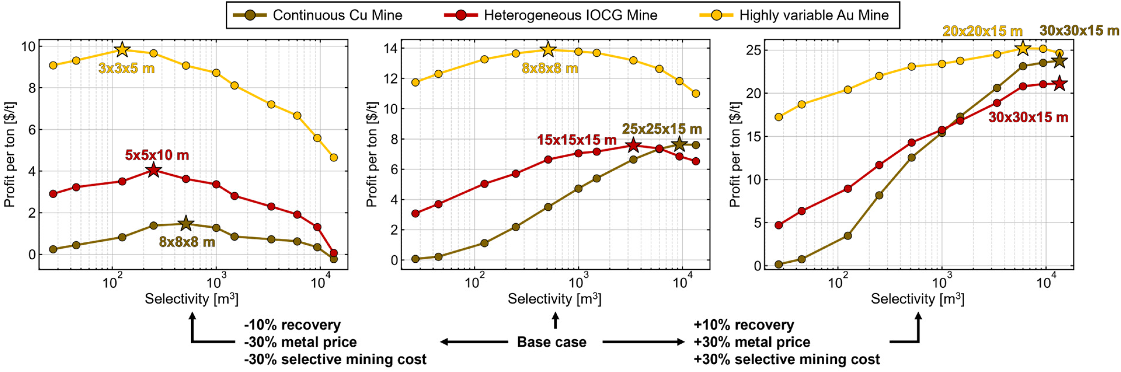
Profit per tonne curves showing the optimal selectivity and drill spacing for the base case and two scenarios which benefit and detract from more selective mining.

Recommendations for drillhole spacing and mining selectivity analysis

The grade control production data is an important input for the simulation of the high resolution ground truth block model to evaluate the different scenarios. Mines which have this data are typically already mature in the extraction stage and the drillhole spacing and mining selectivity optimization workflow can be used to inform decisions in the remainder of the pushback or other areas and pits. If zones with different heterogeneity exist like areas with significant veining, faulting, and folding the workflow should be applied separately from the more uniformly mineralized areas so each is being mined in the most profitable way.

Generating simulations with resolutions which match drillhole samples in large volumes can be computationally demanding for testing large volumes of data. After drawing the drillhole samples the simulated grid in this study was upscaled to 1 × 1 × 1 m which both facilitated the comparison to the eleven scenarios with standard SMU block sizes and reduced the number of points to accelerate the computer processing time. For applications using coarser SMU blocks the grid can be upscaled further if the dataset is too large to be reasonable computed. The number of scenarios can also be reduced and once a local optimum is identified, another set of scenarios can be run at smaller steps from the local optimum.

In this study a wide range of scenarios was run but mines which don’t have a flexible fleet of different digging systems would need to consider the capital expenditure of buying or renting different equipment and the operational impact with considerations for production and asset utilization. The inflexibility of changing mine equipment should help guide the practitioner when choosing which bench height to composite the drillhole samples to which helps constrain the drillhole spacing and mining selectivity scenarios. If decent analogue data exists before fleet decisions are made, the capital and operating expenditures of a higher productivity fleet, more selective fleet, or hybrid fleet can be studied to determine which is ideal.

Conclusions

The developed drillhole spacing and mining selectivity optimization workflow was able to identify an optimal result on distinctly heterogeneous deposits using simple metallurgical, economic, and operating value inputs following industry trends. The workflow also allows the practitioner to decide which and how many scenarios to run while defining the input variables as appropriate for a given site. The example presented here applied the same inputs to eleven drillhole spacing and mining selectivity scenarios from 3 × 3 × 3 m (27 m³) to 30 × 30 × 15 m (13,500 m³). Comparing across deposits spanning extreme homogeneity and heterogeneity demonstrated robust and consistent results with profit differences of the optimum scenario to the next best scenario varying by millions of dollars (1–8%) depending on the grade variability for the three mines.

Future work can focus more on the quantity and direction in which the drillhole samples are taken. In this study the drillhole samples were taken at 90 degrees but this could be varied so the samples are taken perpendicular to the direction of mineralization allowing for a better delineation of the orebody from the waste using less drillholes. Variable drilling densities so more samples are taken along transitions and less in homogeneous areas could also be explored to quantify the potential cost saving.