Similarity and difference in machining at mixed scales using nanostructured coated tools milling hypoeutectoid carbon steel

Abstract

There are similarities and differences when machining at the microscale and macroscale. One difference is the lack of significant heat generated at the microscale, which means that thermal barrier coatings are largely redundant. However, the mechanisms of wear are similar and different depending on machining parameters. In this study, it is discovered that nanostructured coatings play different roles at mixed scales, which are experimentally determined by measuring tool wear, chemical diffusion, temperature, and forces. The main findings show that macroscale wear is thermal in nature and that microscale wear is primarily tribological. The principal conclusions focus on redesigning microtools and nanostructured coatings to eliminate wear, developing standards that describe the action of microtools, and understanding how to calculate the minimum chip thickness that guarantees the formation of chips rather than burrs.

Introduction

Micromilling produces different challenges compared to conventional milling from a material ¹ and a tool wear perspective. ² Therefore, it deserves special consideration. The main reasons for this include size effects (multi-phases and microstructural faults), cutting speed, and the edge radius to depth-of-cut ratio (r_c/h_cu). The size effect occurs with a decrease in scale and the probability of encountering material defects (dislocations/stacking faults and/or grain boundaries) decreases. As a result, the material begins to approach its theoretical strength, that is, a defect-free material. The cutting edge does not experience local changes in the material due to transitions from one grain to the next. ¹ Cutting speed is important at the microscale because material must be machined at its recommended speed, which is the premise for micromilling. Since the tool radius is small, angular velocity must be large. This leads to the third major consideration, the edge radius to depth-of-cut ratio (r_c/h_cu). Owing to high spindle speeds, the depth of cut, or feed per tooth for a milling operation, is often smaller than the edge radius of the tool (f_tooth < r_c). This means that a chip is not always formed during each rotation of the tool. For these reasons, micromilling encounters different problems from macromilling. ³

Burr formation is observed at the macroscale and can contribute ~30% of machining time and cost. Burr formation is also observed at the microscale, but Gillespie ⁴ discovered that macroscale burr removal techniques could not be applied to the microscale. Gillespie and Blotter ⁵ stated that there are three generally accepted burr formation mechanisms: lateral deformation, chip bending, and chip tearing. However, most micro-burr formation studies are at a disadvantage by operating well below the recommended cutting speed, for example machining aluminum with a 50-µm diameter tool demands a cutting speed of 105 m/min, which would require a spindle speed of 670,000 rpm.

At the macroscale, burrs can be quantified owing to both burr height and width can be measured. However, at the microscale, such techniques are difficult to employ. ⁶ Research by Ko and Dornfield ⁷ described a three-stage process for burr initiation, development, and formation. They developed a model of burr formation mechanism that worked well for ductile materials such as Al and Cu. However, at this time, burr formation was not well understood but correlations between machining parameters can identify that up-milling generally creates smaller burrs than down milling. ⁸ It cannot be assumed that if milling is scaled down to the microlevel that machining characteristics will scale similarly. ⁹ During macromachining, the feed per tooth is larger than the cutting edge radius (f_tooth > r_c). However, during micromachining, the feed per tooth is equal to or less than the cutting edge radius (f_tooth ≤ r_c). ¹⁰ Conventional milling tools are designed with slenderness ratios (l/d ~ 2–3), which prevents bending, whereas microtools are susceptible to bending because their diameters are only a few hundred microns. ¹¹ During macroscale cutting, the leading tool edge encounters bulk material (composite structures), and therefore, avoids contact with hard particles, while a microcutting edge encounters individual grains ensuring contact with soft and hard particles. ¹²

The results of Ikawa et al. ¹³ suggest that there is a critical minimum depth of cut below which chips do not form. The analysis of Yuan et al. ¹⁴ indicates that chip formation is not possible if the depth of cut is less than 20%–40% of the cutting edge radius (h_c < (0.2 r_c – 0.4 r_c)). Micromachining at 80,000 rpm produces chips like those created by macroscale machining, where chip curl and helix effects are observed. Kim and Moon ¹⁵ also observed that if the feed rate is too low, a chip is not necessarily formed by each revolution of the tool. This anomaly can be demonstrated by calculation; if the feed rate is low enough, the volume of material removed is predicted to be greater than the volume of chips created. Thus, some rotations that were assumed to create a chip could not have done so. This effect was demonstrated by experimental evidence. Sutherland and Babin ¹⁶ found that feed or machining marks, are separated by a spacing equal to the maximum uncut chip thickness (f_spacing = h_cu). Results at small feeds per tooth show the distance between feed marks is larger than the uncut chip thickness (f_spacing > h_cu), indicating that no chip has been formed. Kim and Moon ¹⁵ conclude that tool rotation without the formation of a chip is due to the combined effects between the ratio of cutting edge radius to feed-per-tooth (r_c/f_tooth) and the lack of rigidity tool of the tool. Work by Ikawa et al. ¹⁷ and Mizumoto et al. ¹⁸ showed single-point diamond turning can machine surface roughness to a tolerance of 1 nm; the critical parameter was found to be repeatability of the depth of cut.

Low cutting forces are produced at the microscale, and so smaller machine structures can achieve the damping and stiffness characteristics required for successful machining. The smaller footprint allows a greater number of machines per unit area yielding a greater throughput and making the technique suitable for mass production. Vogler et al. ¹⁹ examined the differences between macroscale and microscale machining and found that the tool edge and workpiece material grains become comparable in size. The tool edge radius becomes similar in size to the uncut chip thickness (r_c = h_cu) resulting in large plowing forces. Also, the tool’s slenderness ratio (l/d ~ 5) reached a point where tool stiffness is reduced. The force prediction model of Vogler et al., ¹⁹ accounted for different grains such as pearlite and ferrite by examining their individual machining characteristics and incorporating them into the model. Machining characteristics of the bulk material can then be predicted and it was found that cutting edge conditions had a large effect on machining forces. A worn tool edge can produce 300% more cutting force than a sharp edge, resulting in poor surface roughness and increased burr formation.^{5, 7, 9} Cutting conditions of ω = 120,000 rpm, feed per tooth f_tooth = 4 µm, and depth of cut h_c = 100 µm produced a peak cutting force of 3 N. Separations between feed marks were 4 µm and the associated waviness wavelength was 20 µm. ¹⁹ A molecular dynamics model was constructed and it was discovered that when machining aluminum with a diamond tool, chips can only be formed if the minimum depth of cut is approximately half the cutting tool radius (h_{c min} ≈ 0.5 r_c). If the feed per tooth is less than the tool’s edge radius (f_tooth < r_c), the maximum uncut chip thickness does not coincide with the feed per tooth (h_{cu max} ≠ f_tooth), indicating that several rotations are made without the production of a chip. The chip forms when the critical depth of cut is reached.^{20, 21}

The focus of the current work aims to determine: (A) the mechanisms of tool wear in the high-speed micromilling regime and compare them to established macroscale tool wear mechanisms; and (B) whether macroscale tool coatings offer the same degree of function at high-speed on the microscale. The following questions are also considered in this study: is tool wear a barrier to successful mechanical high-speed micromachining? What are the wear mechanisms for coated and uncoated tools at the microscale? Is the wear mechanism the same for an uncoated tool and an uncoated tool at the microscale? What is the most effective tool coating in terms of improving tool life, is it the same coating used at the macroscale? To answer these questions, it is important to understand the characteristics of the operating parameters at the microscale so that they can be compared with the macroscale. The next section focuses on understanding similarities between the two length scales on machining parameters.

Similarity in machining

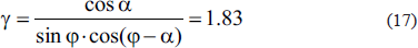
Similarity in machining is a helpful way of describing the differences in measures of performances between mixed scales. In this case, it is interesting to compare between the macroscale and microscales to identify whether nanostructured coatings are necessary for efficient machining at the microscale. ²² The chip compression ratio (ζ) is described as the ability of a material to be machined in terms of intense plastic compression and eventual fracture. The chip compression ratio (ζ) is typically made of ratios of kinematic scalar quantities

$$\text{ζ}=\frac{{\text{l}}_{\text{contact}}}{{\text{l}}_{\text{chip}}}=\frac{{\text{h}}_{\text{c}}}{{\text{h}}_{\text{cu}}}=\frac{\text{v}}{{\text{v}}_{\text{chip}}},$$

(1)

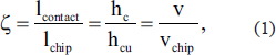
where ζ is the ratio of length of contact l_contact; to the length of the chip formed l_chip; ratio of chip thickness h_c; to the uncut chip thickness h_cu; and the ratio of cutting speed v; to chip velocity v_chip. ζ is a criterion of similarity because work is expended in plastically deforming a unit volume of material

$${\text{A}}_{\text{unit}}=2\text{K}{\left(\text{ln}.\text{ζ}\right)}^{\text{n}+1},$$

(2)

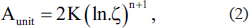
where K is a coefficient related to strength of the material and n is work hardening exponent. For engineering materials at the macroscale, ζ for milling copper alloys ~3–5, aluminum alloys ~2–3.5 and for steel ~2.2–3.3. More heat is generated in steel compared to aluminum and copper alloys and leads to increased tool wear compared to milling copper and aluminum alloys. Micromilling along a fixed boundary is treated as a linear moving heat source and similarity numbers in hot milling use Peclet numbers (Pe) to represent the combined effects of dynamic cutting conditions and thermal responses to the moving heat source over the material. The energy generated in micromilling due to incipient plastic deformation and frictional interactions are used to physically model the process. The Peclet number is

$$\text{Pe}=\frac{\text{v}.{\text{h}}_{\text{c}}}{\text{α}},$$

(3)

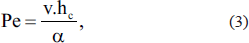
where v is cutting speed, h_c is uncut chip thickness, and α is thermal diffusivity of the workpiece material,

$$\text{α}=\frac{{\text{k}}_{\text{workpiece}}}{{\left(\text{ρ}.{\text{c}}_{\text{p}}\right)}_{\text{workpiece}}},$$

(4)

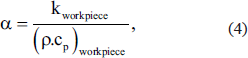
where k_workpiece is the thermal conductivity of the work material, and (c_p·ρ)_workpiece is the volume specific heat of material. When Pe > 10, the thermal energy generated does not change the metallurgical structure of the workpiece material; when milling is cold, the condition of deformation used in modeling cannot be dependent on temperature variations. When Pe < 10, the material is affected by microstructural changes caused by the heat wave propagated at and below the surface of the compressed material. When micromilling is hot, temperature-dependent machining models such as the Johnson-Cook, BCJ, and Zerrelli-Armstrong models can be used for iterative models. For aluminum alloys (ζ ~ 2–3.5), Pe values are typically 60 to 220 at the macroscale, that is, machined cold. The Peclet number Pe depends primarily on ζ and the associated generation of heat governed by progressive plastic compression.^{23, 24}

Another similarity index for micromilling efficiency is defined using the Poletica number (Po), which demonstrates similarity of frictional contact of pairs and requires a knowledge of the uncut chip thickness, rake angle, and the velocity of cut thus,

$$\text{Po}=\frac{{\text{L}}_{\text{chip}}}{{\text{h}}_{\text{cu}}}=\text{f}\left(\text{φ},{\text{ ω}}_{\text{action}}\right),$$

(5)

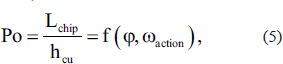
where $\mathrm{\phi }$ is shear plane angle and ω_action is the angle of action. Po is a function of two angles that are directly correlated with each other depending on how the tool enters the workpiece. Clearly,

$$\text{φ}={\text{tan}}^{–1}\left(\frac{\cos \text{γ}}{\text{ζ}–\text{sinγ}}\right),$$

(6)

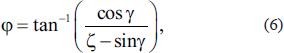
which is related to ζ, or simply stated that Po is directly related to one significant angle and ζ. Po is invariant of the mechanical and physical changes to workpiece materials, which means that strain hardening has no effect on Po or ζ. Machinability of materials is characterized by the ease with which micromilling takes place and is affected by the uncut chip thickness h_cu, and width b, the heat capacity of the materials used, the temperature at which the material is cut and the cutting force criterion,

$$\text{A}=\frac{{\text{h}}_{\text{cu}}{\text{bc}}_{\text{ρ}}{\text{θ}}_{\text{c}}}{{\text{F}}_{\text{p}}}.$$

(7)

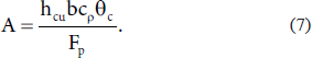
The A-criterion explains the thermal energy absorbed by the materials relative to the total heat generated in the deformation zone, where the A-criterion denotes, c_ρ, as the volumetric heat capacity of the work material measured, θ_c is the cutting temperature, and F_p is the force component of the power developed in the direction of cutting. The D-criterion characterizes the uncut chip cross-section as a function of the true chip width $\mathrm{D}=\frac{{\mathrm{h}}_{\mathrm{c}\mathrm{u}}}{\mathrm{b}}$ . Clearly, at the microscale, the blunting of the cutting tool edge is a significant hinderance to chip formation that leads to an increase in the number of burrs.^4–9 Therefore, the E-criterion is used and describes the relative sharpness of the cutting edge $\mathrm{E}=\frac{{\mathrm{r}}_{\mathrm{c}}}{{\mathrm{h}}_{\mathrm{c}\mathrm{u}}}$ . The E-criterion relates the cutting edge radius r_c with respect to the uncut chip thickness h_cu. The F-criterion characterizes influence of the tool geometry in terms of thermal conductivity of the tool and workpiece materials

$$F=\frac{k_t}{k_w}{\beta }_n{\epsilon }_{tn},$$

(8)

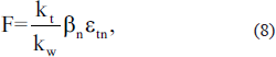
where k_t and k_w are thermal conductivities of tool and workpiece materials, respectively, β_n is normal tool wedge angle, and ε_tn is the nose angle of the tool. To locate the correct angles when micromilling, the tool-in-use notation is used to define the relative positions between angles after the tool has been set in the tool holder. Directions of primary and feed motions may be different from the assumed directions in the tool-in-hand system when the tool is active. Simple relationships exist between angles in the tool-in-hand system and the tool-in-use system. ²⁵ To match the tool-in-use system to the machine reference system, it is important to employ transformation matrices. For a micromilling cutter, it is assumed that the transformation matrix is populated by principal cutting edge angles that are equal to sines and cosines of the principal cutting edge such that A, B, and C = 0 and that when the feed is much less than the circumference of the tool (f << ύd), then the typical transformation matrix ²⁶ is represented by

$$\left[\text{T}\right]=\left[\begin{array}{ccc}\text{cosA}& \text{sinA}& 0\\ –\text{sinA}& \text{cosA}& 0\\ 0& 0& 1\end{array}\right]=\left[\begin{array}{ccc}1& 0& 0\\ 0& 1& 0\\ 0& 0& 1\end{array}\right].$$

(9)

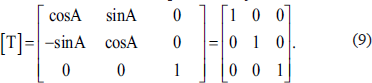
For micromilling, the A, D, E, and F criteria have not normally been calculated or measured. However, Jackson et al.^{10, 11} conducted experiments to begin characterizing similarity measures in micromilling. When micromachining aluminum alloys with 1–3 mm depth(s) of cut, Jackson et al.^{10, 11} noted that the A-criterion ~40–101, D-criterion ~0.3, E-criterion ~1.4–2.67, and F-criterion ~20–454 for coated and uncoated tools.

For the current work based on experimental conditions and calculations, the Peclet number was based on the chip compression ratio, ζ = 1, and was calculated to be 4.5 at 41.5°C and Pe = 4.9 at 142°C. As Pe < 10, the micromilling regime is considered to affect the metallurgical structure of the workpiece. The Poletica number was calculated to be 13.4, A-criterion ~2.5 × 10⁻⁵ at 41.5°C and 8.5 × 10⁻⁵ at 142°C. The D-criterion ~0.05 and E-criterion ~0.6 based on experimental measurements. F-criterion was difficult to estimate due to the variation in angles presented by the tool to the workpiece but was estimated to be ~3410.

Machining analysis

When employing measures of similarity between mixed scales, it is helpful to understand if closed-form solutions and computational methods are useful in characterizing micromilling processing of materials. The following sections describe the calculation of forces and temperatures in micromilling of AISI SAE 1020 hypoeutectoid steel (~0.2 wt.% carbon in iron) using methods described in references.^{10–12, 22, 24, 28, 29}

Closed-form solutions

The feed per tooth ${\mathrm{f}}_{\mathrm{t}\mathrm{o}\mathrm{o}\mathrm{t}\mathrm{h}}=\frac{\mathrm{f}}{\mathrm{n}.\mathrm{N}}$ , f = 25 mm/min = 4.2 mm/s, spindle rotation frequency N = 300,000 rpm, angular velocity ω = 31,416 rad/s, and the number of cutting teeth n = 6. Therefore, f_tooth = 13.9 nm. The feed per tooth correction factor

$${\text{f}}_{\text{tooth correction}}=\frac{{\text{f}}_{\text{tooth}}}{\cos \text{α}}=14\text{ nm.}$$

(10)

However, the edge radius of the cutting tooth is approximately r_c = 3 µm. Therefore, the tool is not sharp enough to form a chip. This has been reported previously by Kim and Moon, ¹⁵ who showed that chips are only formed when the uncut chip thickness is much larger than the edge radius of the tool (h_cu >> r_c). Unfortunately, no exact ratio has been determined. Therefore, it is assumed a chip will form when the uncut chip thickness h_cu reaches 5 µm. This means the tool rotates 360 times before a chip is formed. Thus, the feed per tooth is replaced by the thickness required to form a chip. The rake angle is measured at α = 5°, and the width of cut b is replaced by the axial depth of cut for a milling operation, which in this case is 100 µm. The uncut chip cross sectional $\mathrm{A}={\mathrm{f}}_{\mathrm{t}\mathrm{o}\mathrm{o}\mathrm{t}\mathrm{h}\mathrm{ }\mathrm{c}\mathrm{o}\mathrm{r}\mathrm{r}\mathrm{e}\mathrm{c}\mathrm{t}\mathrm{i}\mathrm{o}\mathrm{n}}$ = 5 × 10⁻¹⁰ m². The tool diameter d = 900 µm, and the total width of cut is 450 µm. The number of teeth engaged in the cut

$${\text{n}}_{\text{cut}}=\frac{\text{n}\left(90+{\text{sin}}^{–1}\left(\frac{2\text{w}–\text{d}}{\text{d}}\right)\right)}{360}=\mathrm{1.5.}$$

(11)

The machinability adjustment factor C_m provided by Isakov ²⁶ ~1 and the tool wear adjustment factor C_w = 1.1. Therefore, the horizontal force ${\mathrm{F}}_{\mathrm{h}}=\mathrm{\sigma }\mathrm{A}{\mathrm{n}}_{\mathrm{c}\mathrm{u}\mathrm{t}}{\mathrm{C}}_{\mathrm{m}}{\mathrm{C}}_{\mathrm{w}}$ = 350 mN. The chip thickness h_c was measured to be 5 µm (h_c = h_cu), thus the chip thickness ratio $\mathrm{r}=\frac{{\mathrm{h}}_{\mathrm{c}}}{{\mathrm{h}}_{\mathrm{c}\mathrm{u}}}=1$ . The shear plane angle

$$\varphi ={\text{tan}}^{–1}\left(\frac{\text{r}.\text{cosα}}{1–\text{r}.\text{sinα}}\right)={47.5}^{°}.$$

(12)

According to Bowden and Tabor, ²⁷ the coefficient of friction between tungsten carbide and low carbon steel µ ~ 0.8. This allows the calculation of the force in the vertical orientation,

$${\text{F}}_{\text{v}}=\frac{\text{μ}.{\text{F}}_{\text{h}}–{\text{F}}_{\text{h}}.\text{tanα}}{1+\text{μ}.\text{tanα}}=230\text{ mN.}$$

(13)

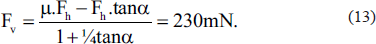
The force along the tool face ${\mathrm{F}}_{\mathrm{a}\mathrm{l}\mathrm{o}\mathrm{n}\mathrm{g}\mathrm{ }\mathrm{t}\mathrm{o}\mathrm{o}\mathrm{l}}={\mathrm{F}}_{\mathrm{h}}.\mathrm{s}\mathrm{i}\mathrm{n}\mathrm{\alpha }+{\mathrm{F}}_{\mathrm{v}}.\mathrm{c}\mathrm{o}\mathrm{s}\mathrm{\alpha }$ = 260 mN. The force normal to the tool face ${\mathrm{F}}_{\mathrm{n}\mathrm{o}\mathrm{r}\mathrm{m}\mathrm{a}\mathrm{l}\mathrm{ }\mathrm{t}\mathrm{o}\mathrm{o}\mathrm{l}}={\mathrm{F}}_{\mathrm{h}}.\mathrm{c}\mathrm{o}\mathrm{s}\mathrm{\alpha }-{\mathrm{F}}_{\mathrm{v}}.\mathrm{s}\mathrm{i}\mathrm{n}\mathrm{\alpha }$ = 330 mN. The force along the shear plane ${\mathrm{F}}_{\mathrm{a}\mathrm{l}\mathrm{o}\mathrm{n}\mathrm{g}\mathrm{ }\mathrm{s}\mathrm{h}\mathrm{e}\mathrm{a}\mathrm{r}}={\mathrm{F}}_{\mathrm{h}}.\mathrm{c}\mathrm{o}\mathrm{s}\mathrm{\phi }-{\mathrm{F}}_{\mathrm{v}}.\mathrm{s}\mathrm{i}\mathrm{n}\mathrm{\phi }$ = 690 mN. The force normal to the shear plane ${\mathrm{F}}_{\mathrm{n}\mathrm{o}\mathrm{r}\mathrm{m}\mathrm{a}\mathrm{l}\mathrm{ }\mathrm{s}\mathrm{h}\mathrm{e}\mathrm{a}\mathrm{r}}={\mathrm{F}}_{\mathrm{v}}.\mathrm{c}\mathrm{o}\mathrm{s}\mathrm{\phi }+{\mathrm{F}}_{\mathrm{h}}.\mathrm{s}\mathrm{i}\mathrm{n}\mathrm{\phi }$ = 410 mN. Since the milling process is being approximated by an orthogonal cutting operation, the milling depth of cut is equal to the width of the chip b. The area of the shear plane

$$A_{\text{shear }}=\frac{b\cdot h_c}{\sin \phi }=6.78\times {10}^{–10}{\text{m}}^2.$$

(14)

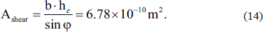
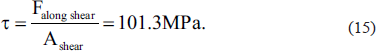
The shear stress

$$\tau =\frac{F_{\text{along shear }}}{A_{\text{shear }}}=101.3\text{MPa}.$$

(15)

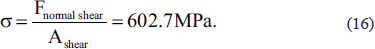
Similarly, the normal stress

$$\sigma =\frac{F_{\text{normal shear }}}{A_{\text{shear }}}=602.7\text{MPa}.$$

(16)

The shear strain

$$\gamma =\frac{\cos \alpha }{\sin \phi \cdot \cos (\phi –\alpha )}=1.83$$

(17)

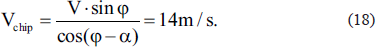
The cutting velocity V_tip = ω.r_tip = 14.1 m/s and chip velocity

$$V_{\text{chip }}=\frac{\text{V}\cdot \sin \phi }{\cos (\phi –\alpha )}=14\text{m}/\text{s}.$$

(18)

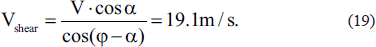
Similarly, the shear plane velocity

$${\text{V}}_{\text{shear }}=\frac{\text{V}\cdot \cos \alpha }{\cos (\phi –\alpha )}=19.1\text{m}/\text{s}.$$

(19)

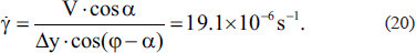
In order to determine the strain rate γ, the shear plane spacing ∇y must be determined from chip images, in this case ∇y = 1 µm. Hence,

$$\dot{\gamma }=\frac{\text{V}\cdot \cos \alpha }{\text{Δy}\cdot \cos (\phi –\alpha )}=19.1\times {10}^{–6}{\text{s}}^{–1}.$$

(20)

The theoretical surface height h_surface, which reflects the surface roughness of the side walls in an end milling operation ${\mathrm{h}}_{\mathrm{s}\mathrm{u}\mathrm{r}\mathrm{f}\mathrm{a}\mathrm{c}\mathrm{e}}=\frac{{\mathrm{f}}^2}{4\mathrm{d}}$ ~ 7 nm. The energy per unit time $\mathrm{U}={\mathrm{F}}_{\mathrm{h}}\mathrm{V}$ = 4.9 J s⁻¹. The energy per unit volume $\mathrm{U}=\frac{{\mathrm{F}}_{\mathrm{h}}}{\mathrm{b}{\mathrm{h}}_{\mathrm{c}}}$ = 695.6 MJ/m³. The shear energy per unit volume ${\mathrm{U}}_{\mathrm{s}\mathrm{h}\mathrm{e}\mathrm{a}\mathrm{r}}=\mathrm{ }\mathrm{\tau }\mathrm{\gamma }$ = 185.7 MJ/m³. The friction energy per unit volume

$${\text{U}}_{\text{friction }}=\frac{{\text{F}}_{\text{across tool }}\cdot \text{r}}{{\text{bt}}_{\text{o}}}=509.9\text{MJ}/{\text{m}}^3\text{. }$$

(21)

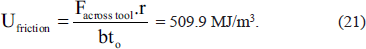
To determine the shear plane temperature, Loewen and Shaw’s method ²⁸ is used and involves several iterations. The initial iteration estimates the shear plane temperature, θ_s = 58°C, while the ambient temperature, θ_o = 25°C. The mean of the two temperatures

$${\theta }_{\text{average }}=\frac{{\theta }_{\text{shear }}+{\theta }_{\text{o}}}{2}={41.5}^{\circ }\text{C.}$$

(22)

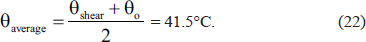
The thermal properties of the workpiece must be determined, and in this case, a low carbon steel. Thermal diffusivity is usually denoted α, but here it is denoted k₁ to avoid confusion with the rake angle also denoted α. At 41.5°C, the thermal diffusivity k₁ = 1.57 × 10⁻⁵ m²/s and the volume specific heat ρ₁C₁ = 3 MJ/m³°C. The thermal quantity

$${\text{R}}_1=\frac{1}{1+1.328{\left(\frac{{\text{k}}_1\gamma }{{\text{Vh}}_{\text{c}}}\right)}^{1/2}}=0.54\text{ and }$$

(23)

$${\theta }_{\text{shear }}–{\theta }_{\text{o}}=\frac{{\text{R}}_1{\text{U}}_{\text{shear }}}{{\text{J}}_{{\rho }_1}{\text{C}}_1}={33.53}^{\circ }\text{C, }$$

(24)

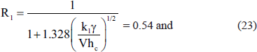
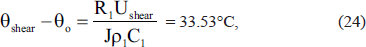
where J is the mechanical equivalent of heat (9340 lb in/BTUs ² for low carbon steel), ~1 Nm/Js ² . Therefore, θs = 58.53°C. Loewen and Shaw ²⁸ state that the iteration should be repeated until the initial estimate produces a shear plane temperature within 3.88°C of the initial estimate. Therefore, in this case, the accepted shear plane temperature is 58.53°C. To calculate the tool face temperature, we must estimate the tool face temperature, θ _{tool face} = 142°C. It is important to determine the thermal properties of the workpiece at this temperature, and in this case, a low carbon steel. At 142°C, k₁ = 1.44 × 10⁻⁵ m²/s, ρ₁C₁ = 3.86 MJ/m³°C. For the macroscale case, the chip contact length, l, was calculated. However, the cutting velocity V is used to derive the formula, and since, it has been established that a chip is not formed at each revolution of the tool at the microscale, applying a formula to find l that is dependent upon V is incorrect. Based on geometrical relationships from the chip contact length $\frac{\mathrm{m}}{\mathrm{l}}=\frac{\mathrm{b}}{2\mathrm{a}}$ = 1.49, from which Ā = 1.2. The thermal conductivity of the workpiece during shearing, k _Shear, at the previously calculated shear plane temperature of 58.53°C, must be determined and in this case k_tool = 6.12 mJ/ms°C. This allows C $\text{'}$ to be calculated where

$$\text{C'}=\frac{{\text{U}}_{\text{friction }}V{T}_{o\overline{A}}}{{\text{Jk}}_{\text{tool }}}=7.07\times {10}^6$$

(25)

B $\text{'}$ is now calculated

$$\text{B'}=\left(\frac{0.754{\text{U}}_{\text{friction }}}{\text{J}{\rho }_{\text{shear }}{\text{C}}_{\text{shear }}}\right){\left(\frac{{\text{Vt}}^2}{\text{ a.r}{\text{.k k}}_{\text{shear }}}\right)}^{1/2}\text{, }$$

(26)

where the subscript s denotes the properties at the previously calculated shear plane temperature of 58.53°C, ρ_sc_s = 3.86 MJ/m³°C and k_s = 1.44 × 10⁻⁵ m/s ² . Therefore,

$$\text{B'}=85.38{\text{ and R}}_2=\frac{\text{C'}–{\theta }_{\text{shear }}+{\theta }_{\text{o}}}{\text{C'}+\text{B'}}=0.99$$

(27)

The temperature rises on the chip’s surface due to friction $\mathrm{\Delta }{\mathrm{\theta }}_{\mathrm{c}\mathrm{h}\mathrm{i}\mathrm{p}}={\mathrm{R}}_2{\mathrm{B}}^{\mathrm{\text{'}}}$ = 85.38°C. Finally, the tool face temperature ${\theta }_{\text{T}}={\theta }_{\text{S}}+\text{Δ}{\theta }_{\text{F}}$ = 143.91°C. Compared to the initial estimate temperature of 142°C, the computed estimated error ~1.91°C. Shaw ²⁹ states the error should be zero. However, since the thermal properties are being determined by graphical means, an error of 1.91°C is considered accurate.

Computational method

A set of finite element algorithms is specifically designed for analyzing micromilling processes based on Lagrange-Euler equations that adaptively re-mesh during the milling operation. ¹⁶ Multi-body deformations simulate micromilling tool-surface interactions with time-dependent thermal effects. Finite deformation kinematics and kinetics include the transfer of momentum and surmounting thermal barriers employing the second law of thermodynamics. ²² The workpiece mesh is an amalgam of tetrahedral-shaped finite elements. A minimum element size of 1 µm and a maximum of 1 mm were used for the cutting tool. The minimum size is used in the region analyzed adjacent to the tool tip owing to the highest level of plastic strain and thermal gradients. The sizes of workpiece elements were 0.015 mm and 0.1 mm, respectively. The power law constitutive model employed ²⁴ $\mathrm{\sigma }\left(\mathrm{\epsilon },\mathrm{ }\dot{\mathrm{\epsilon },\mathrm{ }\mathrm{T}}\right)=\mathrm{g}\left(\mathrm{\epsilon }\right).\mathrm{\Gamma }\left(\dot{\mathrm{\epsilon }}\right).\mathrm{\theta }\left(\mathrm{T}\right)$ , where σ is the yield stress, ε, the plastic strain, $\dot{\mathrm{\epsilon }}$ , the strain rate, T, the temperature, g(ε), the strain hardening behavior of the material, Γ( $\dot{\mathrm{\epsilon }}$ ), the strain rate sensitivity, and θ(T) is the thermal softening parameter. A staggered procedure is used to couple thermal and mechanical meshes. Forward Euler algorithms are integrated into the model, which means that temperature is initialized, an isothermal physical step is implemented, heat is generated at the contact interfaces, and conduction is performed until the cycle is repeated. The initial temperature of the contact system ~20°C. Temperatures reached in micromilling processes affect kinetic responses and are described using the first law of thermodynamics expressed for the system^22–29

$${{\displaystyle \int }}_{\text{Bt}}\rho \text{cT}\eta \text{dV}+{{\displaystyle \int }}_{\partial \text{Btq}}\text{h}\eta \text{dS}={{\displaystyle \int }}_{\text{Bt}}\text{q}\cdot \nabla \eta \text{dV}+{{\displaystyle \int }}_{\text{Bt}}\text{s}\eta \text{dV},$$

(28)

where ρ is the mass density, c, the heat capacity, T, the temperature, η, the admissible virtual temperature, V, the volume, h, the heat flux through the surface, q, the heat flux, s, the distributed heat density, $\nabla$ , the material gradient, and B_tq is the Neumann boundary. Heat generated by plastic deformation is dynamic and the rate of heat $\mathrm{s}=\mathrm{\beta }.\dot{{\mathrm{W}}^{\mathrm{p}}}$ , where Ẇ^p denotes energy used per unit time to deform unit volume of material and β is plastic deformation coefficient. Heat generated at the contact interface is partitioned to the tool and the workpiece as the ratio of heat supplied to the cut chip h₁, and tool h₂, using quasi transient half-space methods, $\frac{{\mathrm{h}}_1}{{\mathrm{h}}_2}=\frac{\sqrt{{\mathrm{k}}_1{\mathrm{\rho }}_1{\mathrm{c}}_1}}{\sqrt{{\mathrm{k}}_2{\mathrm{\rho }}_2{\mathrm{c}}_2}}$ , where k, ρ, and c are thermal conductivity, mass density, and heat capacity of the chip and cutting tool surfaces. Finite element interpolations result in a semi-discrete system satisfying Fourier’s law of heat conduction $\mathrm{C}\dot{\mathrm{T}}+\mathrm{K}\mathrm{T}=\mathrm{Q}$ , where T is an array of temperature nodes, $\dot{\mathrm{T}}$ is an array of temperature rates, Q is heat, K is a constant, C denotes lumped capacitance matrix, and the resultant heat capacity matrix, such as, ${\mathrm{C}}_{\mathrm{a}\mathrm{b}}=\underset{\mathrm{B}\mathrm{t}}{\int }\mathrm{c}\mathrm{\rho }{\mathrm{N}}_{\mathrm{a}}{\mathrm{N}}_{\mathrm{b}}\mathrm{d}{\mathrm{V}}_{\mathrm{o}}$ . The heat conductivity matrix ${\mathrm{K}}_{\mathrm{a}\mathrm{b}}=\underset{\mathrm{B}0}{\int }{\mathrm{D}}_{\mathrm{i},\mathrm{j}}{\mathrm{N}}_{\mathrm{a},\mathrm{i}}{\mathrm{N}}_{\mathrm{b},\mathrm{j}}\mathrm{d}\mathrm{V}$ is provided such that the heat source assumed in the chip or at the tool surface generates a value of heat transfer coefficient, where

$$Q_a={{\displaystyle \int }}_{Bt}s{N}_{a}dV+{{\displaystyle \int }}_{B\tau q}h{N}_{a}dS.$$

(29)

For non-static conditions, the transfer of heat is derived using the second law of thermodynamics and the integral is solved using the forward Euler algorithm T_n+1 = T_n + ∇t $\dot{\mathrm{T}}$ _n, which becomes the equation of the first law of thermodynamics in discrete terms such that $\mathrm{C}\dot{{\mathrm{T}}_{\mathrm{n}+1}}+\mathrm{K}{\mathrm{T}}_{\mathrm{n}+1}={\mathrm{Q}}_{\mathrm{n}+1}$ . For steady-state kinematic conditions, the transition of the non-complex momentum condition is given by ${\mathrm{\sigma }}_{\mathrm{i}\mathrm{j},\mathrm{j}}+\mathrm{\rho }{\mathrm{b}}_{\mathrm{i}}=\mathrm{\rho }\ddot{{\mathrm{u}}_{\mathrm{i}}}$ . The virtual work principle is applied to the transition: $\underset{\mathrm{B}}{\int }{\mathrm{v}}_{\mathrm{i}}{\mathrm{\sigma }}_{\mathrm{i}\mathrm{j},\mathrm{j}}+{\mathrm{v}}_{\mathrm{i}}\mathrm{\rho }{\mathrm{b}}_{\mathrm{i}}\mathrm{d}\mathrm{V}=\mathrm{ }\underset{\mathrm{B}}{\int }\mathrm{\rho }{\mathrm{v}}_{\mathrm{i}}\ddot{{\mathrm{u}}_{\mathrm{i}}}\mathrm{d}\mathrm{V}$ , and when integrated by parts provides a balance of forces for the enclosed system

$${{\displaystyle \int }}_B\rho v_i{\ddot{u}}_{1}dV+{{\displaystyle \int }}_B{v}_{i,j}{\sigma }_{i,j}dV={{\displaystyle \int }}_{\partial B}{v}_i{\sigma }_{i,j}{n}_{j}d\text{Ω}+{{\displaystyle \int }}_B{v}_i\rho b_{i}dV.$$

(30)

The inertial terms plus internal forces are equal to the external forces plus internal forces acting on and within the body of elements

$${\text{Ma}}_{\text{a}+1}+{\text{R}}_{\text{n}+1}^{\text{int}}={\text{R}}_{\text{n}+1}^{\text{ext}}{\text{ and M}}_{\text{ab}}={{\displaystyle \int }}_{\text{B}0}{\rho }_0{\text{N}}_{\text{a}}{\text{N}}_{\text{b}}{\text{dV}}_{\text{o}}$$

(31)

where M_ab is the mass matrix and the external body force array R_ia is ${\mathrm{R}}_{\mathrm{i}\mathrm{a}}^{\mathrm{e}\mathrm{x}\mathrm{t}}=\underset{\mathrm{B}0}{\int }{\mathrm{b}}_{\mathrm{i}}{\mathrm{N}}_{\mathrm{a}}\mathrm{d}{\mathrm{V}}_{\mathrm{o}}+\underset{\partial \mathrm{B}0\mathrm{\tau }}{\int }{\mathrm{\tau }}_{\mathrm{i}}{\mathrm{N}}_{\mathrm{a}}\mathrm{d}{\mathrm{\Omega }}_{\mathrm{o}}$ . The internal force array of the elements is ${\mathrm{R}}_{\mathrm{i}\mathrm{a}}^{\mathrm{i}\mathrm{n}\mathrm{t}}=\underset{\mathrm{B}\mathrm{O}}{\int }{\mathrm{P}}_{\mathrm{i},\mathrm{j}}{\mathrm{N}}_{\mathrm{a},\mathrm{j}}\mathrm{d}{\mathrm{V}}_{\mathrm{o}}$ , where N_a,j denotes shape functions of repeated indices, the comma representing a partial differentiation with respect to spatial coordinate(s), and P_i,j is the nominal “Piola-Kirchhoff” stress tensor for the matrix of elements.^{10, 11}

Experimental methods

Cutting tool wear progression, forces, and temperatures were collected using micromilling tools both coated (TiN, TiCN, CrN, TiAlN (3 grades of this coating are used, their compositions are TiAlN (50% wt. Al/50% wt. Ti), TIAlN (60% wt. Al/40% wt. Ti), TiAlN (70% wt. Al/30% wt. Ti), TiAlN/WC/C, WC/C) and uncoated. The experimental data was compared with closed-form solutions and computational predictions of forces and temperature. The experiments involved removing a prescribed volume of material, measuring experimental variables and then photographing the condition of cutting edges using an optical microscope. This provides a quantitative way to measure wear rate and a qualitative assessment of wear mechanisms. X-ray fluorescence (XRF) was used to provide a relative measure of chemical elements detected in the tool, or the chip, to indicate whether, or not, diffusion of atoms has taken place between the cutting tool and the workpiece.

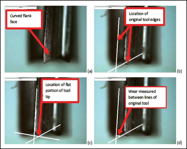
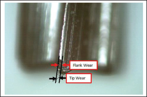
Considering tool wear, ISO 8688 “Tool Life Testing in Milling - Part 2: End Milling” is the international standard used to assess tool wear for milling. ³⁰ This standard identifies several wear mechanisms that can occur during machining such as edge chipping or thermal cracking. At the microscale, the wear criteria of ISO 8688 are not easily adapted. If the ISO 8688 wear criterion ³⁰ is scaled in proportion from a 25.4-mm diameter tool and 300 µm of flank wear to a 900-µm diameter tool, then a flank wear of 10.6 µm would be required for the tool to reach the wear criterion. A pilot study showed 10–20 µm of wear occurs after a small amount of cutting, this makes it an impractical wear criterion to employ. The pilot study also showed that above 100 µm of flank wear cutting was inconsistent since the cutting teeth no longer retain the geometry required for chip formation; this leads to increased bending and eventual fracture of the tool. Therefore, the wear criterion must be set between 20 and 100 µm of flank wear, and 80 µm is tentatively chosen. The suitability of this value will be evaluated at the conclusion of the microscale experiments. Figure 1 shows how microtool wear is evaluated. A new microtool is shown in Figure 1(a), after machining the tool tip is worn away. Therefore, the edges of the original tool geometry must be identified (Figure 1(b)). Wear is then measured along the flat plane of the tool tip as shown in Figure 1(c), and between the two lines identifying the original tool edges as shown in Figure 1(d).

Figure 1.

The measurement of micromilling tool wear: (a) virgin tool showing curved flank face, (b) location of original tool edges on tool, (c) identification of flat portion of tool tip, and (d) wear measured between lines of the original tool location.

Since chemical wear is the result of atomic diffusion, a measurement technique capable of identifying elemental changes is required. XRF analysis was selected for this task since alternative methods of chemical analysis, such as Energy Dispersive X-ray (EDX) microanalysis, or Electron Backscatter Diffraction (EBSD), are usually performed in a scanning electron microscope. If chemical wear occurs, diffusion of the coating into the chips is expected and the amount of tool material detected in the chips would increase. XRF analysis was performed on a virgin micromilling cutter and allows a comparison of the tool composition before, during and after the experimental work. Chips from each experiment were collected at each inspection point of the tool. XRF analysis was performed on all chips collected.

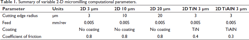
Computational analysis of temperature and micromilling forces was conducted using a Lagrange-Euler formulated finite element algorithm using the variable parameters shown in Table 1. The constant parameters used in the analysis include the workpiece height (0.5 mm), workpiece length (5 mm), workpiece material (AISI 1020 steel), tool material (WC +Co), rake angle (5°), relief angle (10°), depth of cut (1 mm), length of cut (3 mm), cutting speed (6 m/min), and the initial temperature of cut (20°C).

Table 1.

Summary of variable 2-D micromilling computational parameters.

Parameter	Units	2D 3 µm	2D 10 µm	2D 20 µm	2D TiN 3 µm	2D TiAlN 3 µm
Cutting edge radius	µm	3	10	20	3	3
Feed	mm/rev	0.005	0.005	0.005	0.005	0.005
Coating		No coating	No coating	No coating	TiN	TiAlN
Coefficient of friction		0.8	0.8	0.8	0.4	0.3

Experimental apparatus

Figure 2 shows the general arrangement of the experimental apparatus. The original spindle on the micro-milling machine has been replaced with a fixture that allows an air powered high-speed spindle to be used on the machine. Since air spindles are susceptible to failure, the fixture is designed for rapid spindle replacement; an undamaged unloaded spindle should operate at approximately, N = 400,000–410,000 rpm. The micromachine tool was located on a large granite surface plate providing a large mass that rapidly attenuates regenerative vibrations. These precautions are taken to ensure that the micromachine tool is dynamically and kinematically stable. The experimental parameters chosen to produce tool wear suitable for this study are tool diameter d = 900 µm, spindle rotation frequency N = 400,000 rpm (unloaded); feed rate f = 20 mm/min, milling depth of cut b = 100 µm, and width of cut w = 450 µm. The workpiece material (AISI 1020 steel) was chosen since it is a common engineering material, is soft (HRC = 20), and contains a high percentage of ferrite grains. Micromilling forces in orthogonal directions (x and y) were measured with the aid of a Kistler^TM x-y-z-direction (–3 to 6 kN range in all principal axes) dynamometer (Model 9121, charge amplifier model 5070 connected to 2825A-02 sampling software). Small dynamic changes are measured with large force disturbances within the rigid structure (~600 N/µm). Active cutting forces independent of the type of tool used is mounted on quartz sensors. Models for calculating temperature during micromilling integrate thermodynamic principles with the thermal properties of tool, workpiece, and chip.^{28, 29}

Figure 2.

(a) Experimental apparatus: (1) micromilling machine, (2) air turbine, (3) vise and workpiece, (4) magnetic chip collector, and (5) protective screen. (b) Micromiling arrangement: (1) air turbine spindle, (2) micromilling tool, (3) workpiece material, (4) vise, and (5) chips.

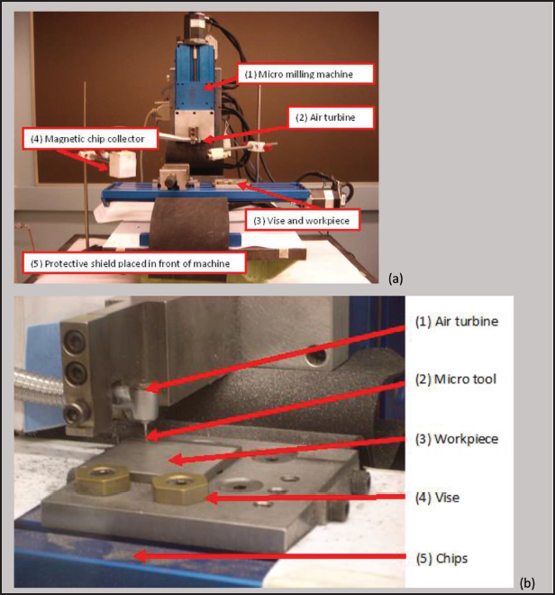
The measurement of cutting temperature at the microscale was measured using the Fluke model Ti 45 infra-red (IR) thermal imaging camera. ¹¹ The camera measures temperatures to 1200°C using a 1024 × 786-pixel resolution grating and a thermal sensitivity of 50 mK (spatial resolution ~0.8 mRad and 1200:1 distance to spot). The camera was connected to the computer through a composite video card, while an Osprey capture card was used to freeze dynamic thermal images. ¹⁰ The camera was directed at the tip of the cutting tool and the maximum temperature was recorded during machining experiments.

Experimental results

Computational methods

A unique problem in computing high-speed micromilling, is that the ratio of the tool edge radius to depth of cut becomes a problem for effective chip formation. The ultra-high spindle speed means that the feed per tooth, or depth of cut when translated from the 3D machining case to orthogonal cutting, is much less than the tool edge radius. Simulations using the exact machining parameters show that no cutting takes place, or if chips are formed then the large tool radius acts as an extreme negative rake angle cutter. ³¹ Eventually, the cumulative movement of the workpiece reaches a critical distance and it has been estimated that a new microtool with an edge radius r_c = 3 µm has a minimum uncut chip thickness h_cu ~ 5 µm.

Microscale computation: 2D milling with an uncoated tool of 3-µm edge radius

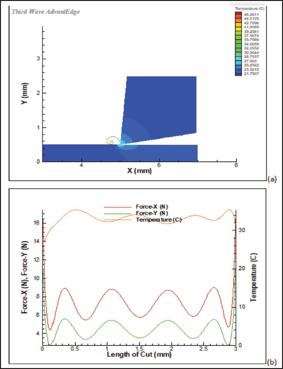
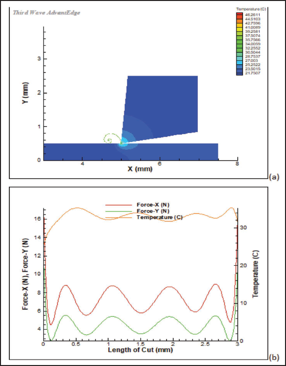
The computation for a single tooth of the micromilling cutter represents 2D macro up-milling. Figure 3 shows the temperature distribution, the peak tool temperature, and forces generated in the x- and y-orientations computed using the edge radius of 3 µm for an uncoated tool. This computation is essentially the control variable for a microscale uncoated tool.

Figure 3.

Microscale 2D computation: (a) temperature field and (b) forces for an uncoated tool with 3-µm edge radius. Simulation parameters are shown in Table 1.

Microscale computation: 2D milling with an uncoated tool of 10-µm edge radius

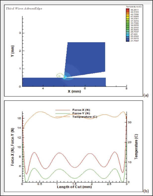
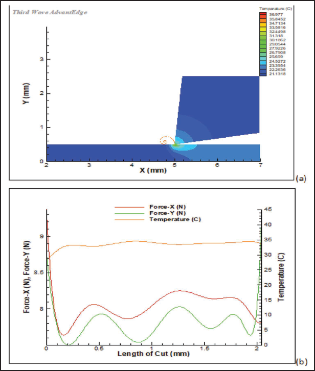
To account for a worn tool, the edge radius of the tool was increased from 3 µm to 10 µm; all other computational parameters were identical (Figure 4).

Figure 4.

Microscale 2D computation: (a) temperature field and (b) forces for an uncoated tool with 10-µm edge radius. Simulation parameters are shown in Table 1.

Microscale computation: 2D milling with an uncoated tool of 20-µm edge radius

To account for a worn tool, the edge radius of the tool was increased from 3 µm to 20 µm; computational parameters are shown in Table 1 and results are shown in Figure 5.

Figure 5.

Microscale 2D computation: (a) temperature field and (b) forces for an uncoated tool with a 20-µm edge radius. Simulation parameters are shown in Table 1.

Microscale computation: 2D milling with a TiN coated tool of 3-µm edge radius

To account for a coated tool, the tool was coated with a 3-µm thick TiN coating; all other computational parameters were identical. The computation results are shown in Figure 6.

Figure 6.

Microscale 2D computation: (a) temperature field and (b) forces for a TiN coated tool with a 3-µm edge radius. Simulation parameters are shown in Table 1.

Microscale computation: 2D milling with a TiAlN coated tool of 3-µm edge radius

To account for a coated tool, the tool discussed was coated with a 3-µm thick TiAlN coating and the results are shown in Figure 7.

Figure 7.

Microscale 2D computation: (a) temperature field and (b) forces for a TiAlN coated tool with a 3-µm edge radius. Simulation parameters are shown in Table 1.

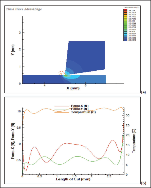
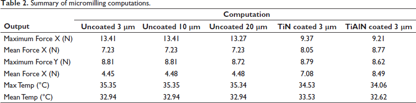
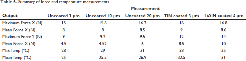
There is very little variation in the forces or temperatures for any of the computational conditions (Figures 3–7, Table 2). Changing the edge radius had virtually no effect on the results. However, TiN and TiAlN coatings did affect the results. The coatings reduced the peak x-force by approximately 4 N but increased the mean force by 1 to 1.5 N. The peak y-force was about the same for all computations, ~4.5 N, but the TiN coating increased the mean y-force by 3.6 N and the TiAlN coating by 4 N. The coatings reduced the peak temperature of approximately 35.35°C by 1°C. However, TiN coating caused the mean temperature of 32.94°C to increase ~0.6°C. There is little variation between computational results. Therefore, from a computational viewpoint, it appears that coatings at the microscale have very little effect on micromachining results.

Table 2.

Summary of micromilling computations.

	Computation
Output	Uncoated 3 µm	Uncoated 10 µm	Uncoated 20 µm	TiN coated 3 µm	TiAlN coated 3 µm
Maximum Force X (N)	13.41	13.41	13.27	9.37	9.21
Mean Force X (N)	7.23	7.23	7.23	8.05	8.77
Maximum Force Y (N)	8.81	8.81	8.72	8.79	8.62
Mean Force X (N)	4.45	4.48	4.48	7.08	8.49
Max Temp (°C)	35.35	35.35	35.34	34.53	34.06
Mean Temp (°C)	32.94	32.94	32.94	33.53	32.62

Micromachining results

Subsections “CrN coated tool” to “Uncoated coated tool” describe the XRF chemical analysis results, where relevant tables are used to show the chemical composition of the tool or chips. Typical images of tool wear for each coating are also included including line diagrams of flank wear against volume removed for each coating, while tool wear images are superimposed on the diagrams to demonstrate how tool wear progresses. The wear mechanism is identified from Figure 8 as flank wear and is plotted against the volume removed for each tool; a linear trend line with a zero intercept is then determined, the gradient of which is a measure of tool wear. For a given amount of flank wear the theoretical workpiece volume removed is calculated from the linear trend line. The results are presented in the random order in which the experiments were conducted.

Figure 8.

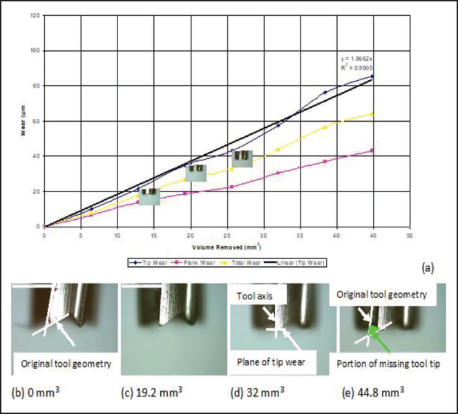
Volume of workpiece material removed as a function of wear of CrN coated micromilling tool: (a) characteristic wear curve, (b) original tool geometry before machining, (c) tool wear after machining 19.2 mm³ of workpiece, (d) tool wear after machining 32 mm³ of workpiece, and (e) tool wear after machining 44.8 mm³ of workpiece material.

CrN coated tool

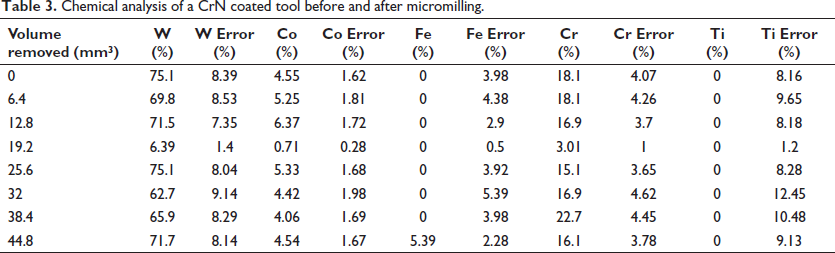
The XRF chemical analysis of the tool detected a deposit of iron (~5.39%) on the tool when it is declared worn (Table 3). The amount of tungsten detected is variable between 62.7% and 75.1% and is due to the misidentification of aluminum (not shown in the table). Occasionally, a large amount of aluminum is detected which skews the relative percentage of each element detected, this occurred at a volume removed of 19.2 mm³ and is not considered significant. No coating material was detected on the chips. Therefore, it can be concluded that there is no evidence of chemical wear. Figure 8 shows selected images of the typical progression of wear on tooth number two.

Table 3.

Chemical analysis of a CrN coated tool before and after micromilling.

Volume removed (mm3)	W (%)	W Error (%)	Co (%)	Co Error (%)	Fe (%)	Fe Error (%)	Cr (%)	Cr Error (%)	Ti (%)	Ti Error (%)
0	75.1	8.39	4.55	1.62	0	3.98	18.1	4.07	0	8.16
6.4	69.8	8.53	5.25	1.81	0	4.38	18.1	4.26	0	9.65
12.8	71.5	7.35	6.37	1.72	0	2.9	16.9	3.7	0	8.18
19.2	6.39	1.4	0.71	0.28	0	0.5	3.01	1	0	1.2
25.6	75.1	8.04	5.33	1.68	0	3.92	15.1	3.65	0	8.28
32	62.7	9.14	4.42	1.98	0	5.39	16.9	4.62	0	12.45
38.4	65.9	8.29	4.06	1.69	0	3.98	22.7	4.45	0	10.48
44.8	71.7	8.14	4.54	1.67	5.39	2.28	16.1	3.78	0	9.13

The type of wear observed in Figure 8 matches the description of uniform flank wear. However, it does not occur along the tool flank, instead the entire tool tip is eroded in a plane perpendicular to the tool’s axis. There is wear along the tool flank although this is considered a minor feature in comparison to the wear of the tool tip. Figure 9 shows the original location of the tool edge at a volume removed of 0 mm³, the plane of tip wear is shown at a volume removed of 32 mm³, and the portion of the tool tip worn away is shown at a volume removed of 44.8 mm³. This type of wear will be referred to as tip wear. The wear criterion of 80 µm is achieved at a volume removed of 42 mm³. Experimentally, the criterion of wear was reached at a volume removed of 41 mm³, after that, the tool tip started to break away due to concentrated fracture at the tool tip.

Figure 9.

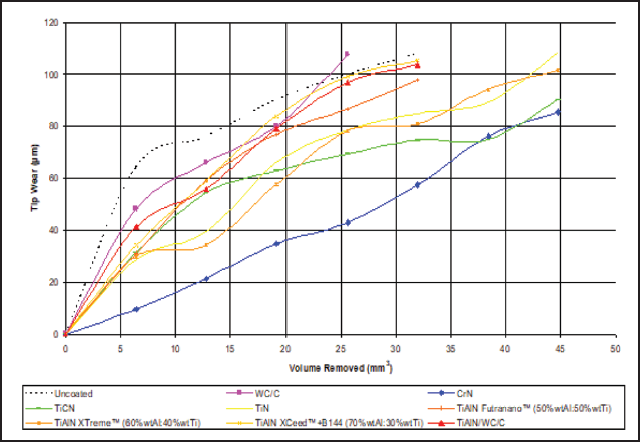
Wear of micromilling tool tip as a function of the volume of workpiece material removed for all micromachining experiments.

TiN coated tool

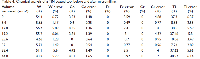
The XRF chemical analysis of the tool produced highly variable results, but no deposits of iron were detected (Table 4). The amount of tungsten detected was between 5.5% and 75.1%. This is due to the misidentification of aluminum. It is likely that the combination of complex geometry and the small surface area of the tool available for sampling contributes to this effect. Therefore, XRF chemical analysis of the tool proved inconclusive. However, XRF analysis detected no coating material in the chips. Therefore, it can be concluded that there was no evidence of chemical wear by diffusion.

Table 4.

Chemical analysis of a TiN coated tool before and after micromilling.

Volume removed (mm3)	W (%)	W error (%)	Co (%)	Co error (%)	Fe (%)	Fe error (%)	Cr (%)	Cr error (%)	Ti (%)	Ti error (%)
0	54.4	6.72	3.53	1.48	0	3.59	0	4.88	37.3	6.37
6.4	5.55	1.17	0.6	0.25	0	0.49	0	0.77	8.33	2.53
12.8	56.7	5.89	4.35	1.36	0	2.41	0	4	38.5	5.59
19.2	55.2	6.06	3.84	1.39	0	3.1	0	4.32	37.46	5.8
25.6	4.66	1.28	0	0.64	0	0.7	0	0.95	10.06	3.49
32	5.71	1.49	0	0.54	0	0.77	0	0.96	7.24	2.89
38.4	51.1	5.6	4.42	1.49	0	3.51	0	4	37.62	5.66
44.8	43.2	5.79	4.01	1.65	0	3.92	0	2	48.97	6.14

The type of wear is identified as tip wear, there is also a small amount of flank wear. The wear criterion of 80 µm is achieved at a workpiece volume of 30.65 mm³ removed. Experimentally, wear was reached at a volume removed of 26 mm³.

WC/C coated tool

The XRF chemical analysis of the tool proved to be highly variable and was considered inconclusive. However, no deposits of iron were detected on the tool and no tool material was detected in the chips. Therefore, it can be concluded that there was no evidence of chemical wear. The type of wear was identified as tip wear, and there is also a small amount of flank wear. Based on the linear trend line, wear of 80 µm is achieved at a volume of 18.05 mm³ removed. Experimentally, wear by attrition was reached at a volume removed of 19 mm³.

TiAlN/WC/C coated tool

The XRF chemical analysis of the tool was highly variable and proved to be inconclusive. However, no iron deposits were detected on the tool. The chips showed no evidence of that tool material had diffused into them. Therefore, it can be concluded that there was no evidence of chemical wear. The type of wear was identified as tip wear, and there is also a small amount of flank wear. The wear criterion is achieved at a volume of 21.71 mm³ removed. Experimentally, wear was reached at a volume removed of 19 mm³.

TiAlN (60% wt. Al:40% wt. Ti) coated tool

The XRF chemical analysis showed a small variation in the amount of tungsten and titanium detected (Table 5). The most significant difference was seen at 0 mm³ removed, the reason for this is unclear. No tool material was detected in the chips. Therefore, it can be concluded that there was no evidence of chemical wear.

Table 5.

Chemical analysis of a TiAlN (60% wt. Al:40% wt. Ti) coated tool before and after micromilling.

Volume removed (mm3)	W (%)	W error (%)	Co (%)	Co error (%)	Fe (%)	Fe error (%)	Cr (%)	Cr error (%)	Ti (%)	Ti error (%)
0	5.57	1.45	0.63	0.31	0	0.65	0	0.71	5.38	2.6
6.4	67.6	8.61	4.12	1.63	0	3.62	0	4.67	24.73	6.98
12.8	66.6	8.5	4.78	1.71	0	3.59	0	5.27	22.11	6.88
19.2	70	9.9	5.17	1.94	0	4.29	0	5.6	19.29	7.43
25.6	65.2	9.34	7.25	2.21	0	4.21	0	5.46	25.7	7.5
32	61.7	8.51	4.49	1.83	0	4.72	0	5.88	22.6	7.26
38.4	68.8	9.22	5.02	1.77	0	3.65	0	5.67	22.79	7.12
44.8	63.7	8.8	5.69	2.01	0	4.71	0	3.73	21.86	7.27

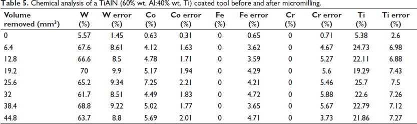
The type of wear was identified as tip wear, and there is also a small amount of flank wear. Based on the linear trend line, wear of 80 µm is achieved at a volume of 31.62 mm³ removed. Experimentally, wear was reached at a volume removed of 31 mm³. Thereafter, the tool tip fractured.

TiAlN (70% wt. Al:30% wt. Ti) coated tool

The XRF chemical analysis was highly variable and proved to be inconclusive; no iron deposits were detected on the tool and no tool material was detected in the chips. Therefore, it can be concluded that there was no evidence of chemical wear by diffusion. The type of wear was identified as tip wear, and there is also a small amount of flank wear. The wear criterion (80 µm) is achieved at a volume of 21.21 mm³ removed. Experimentally, this wear was reached at a volume removed of 18 mm³.

TiAlN (50% wt. Al:50% wt. Ti) coated tool

The XRF chemical analysis was highly variable and proved inconclusive; no iron deposits were detected on the tool and no tool material was detected in the chips. Therefore, it can be concluded that there was no evidence of chemical wear by diffusion. The type of wear was identified as tip wear, and there is also a small amount of flank wear. Wear of 80 µm total loss is achieved at a volume of 25.15 mm³ removed. Experimentally, wear was reached at a volume removed of 21 mm³.

TiCN coated tool

The XRF chemical analysis was highly variable and proved inconclusive; no iron deposits were detected on the tool and no tool material was detected in the chips. Therefore, it can be concluded that there was no evidence of chemical wear by diffusion. The type of wear was identified as tip wear, and there is also a small amount of flank wear. Experimentally, wear was reached at a volume removed of 41 mm³.

Uncoated coated tool

The XRF chemical analysis was highly variable and proved to be inconclusive; no iron deposits were detected on the tool and no tool material was detected in the chips. Therefore, it can be concluded that there was no evidence of chemical wear. The type of wear was identified as tip wear. By inspection, criterion of wear is achieved at a volume of 19.74 mm³ removed. Experimentally, wear was reached at a volume removed of 14.5 mm³. Table 6 shows the results of maximum and mean forces and maximum and mean temperature measurements for a selection of tool and coating thickness measured during the micromilling experiments. Forces were measured using a dynamometer and temperatures measured using the thermal imaging camera.

Table 6.

Summary of force and temperature measurements.

	Measurement
Output	Uncoated 3 µm	Uncoated 10 µm	Uncoated 20 µm	TiN coated 3 µm	TiAlN coated 3 µm
Maximum Force X (N)	15	15.6	16.2	16	16.8
Mean Force X (N)	8	8	8.5	9	8.6
Maximum Force Y (N)	9	9.2	9.5	12	14
Mean Force X (N)	4.5	4.52	6	8.5	10
Max Temp (°C)	28	29	31	38	35
Mean Temp (°C)	25	25.5	26.9	32.5	31

Discussion

For microscale experiments, XRF analysis was conducted directly on the tool and chips. Results for the tools proved to be highly variable owing to the small area available for sampling and the complex geometry of the tool. No deposits of iron were detected on the tool. No coating material was detected in the chips, indicating that there was no diffusion of chemical species from tool-to-chip and vice versa (Tables 3–5). Figure 9 shows micromilling results for all coatings. There is no obvious pattern that distinguishes the wear of the coatings. The uncoated tool exhibits the most rapid wear, whilst the CrN coated tool exhibits the slowest wear progression (Figure 8). The general trend shows a rapid initial wear rate followed by a sustained period at a reduced wear progression.

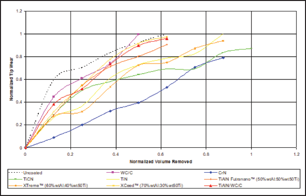
For comparison to the macroscale, results are normalized and shown in Figure 10. The x-axis was normalized against a maximum volume removed of 51.2 mm³ and the y-axis was normalized against a maximum flank wear of 108.18 µm. At the macroscale, two experiments were performed, one termed ‘interrupted cut’ and one termed ‘continuous cut’, this was done to check that the procedure of examining the tool for wear did not affect the experimental results.

Figure 10.

Normalized wear of micromilling tool tip as a function of the volume of workpiece material removed for all micromilling tools.

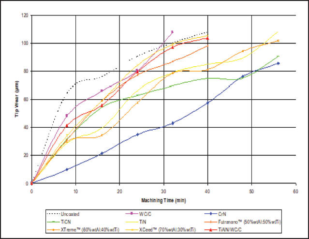
To compare the stages of wear and the wear rates to the macroscale, the microscale results are shown as tip wear against machining time (Figure 11). It can be seen from Figure 12 (TiCN coated tool) that there is no stage three wear. There is a rapid period of initial wear for TiCN coated tools followed by a decrease in wear. For all tools, stage one is identified after eight minutes of machining from the wear images. Figure 12 shows how wear stages one and two are identified, one vertical line is drawn at eight minutes and the second vertical line is drawn at the end of the machining time. The lines of correlation are then added so that the gradient, or wear rate can be determined. However, the R² values for stage II wear are of such magnitude that linear models are considered accurate.

Figure 11.

Wear of micromilling tool tip as a function of machining time for all micromilling tools.

Figure 12.

Identification of the stages of wear using a cut-off value and gradients for a TiCN coated micromilling tool.

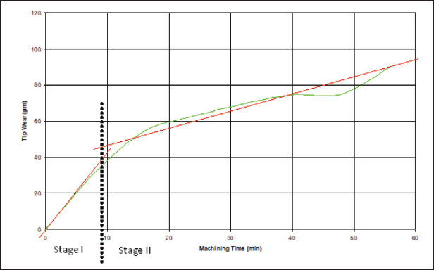
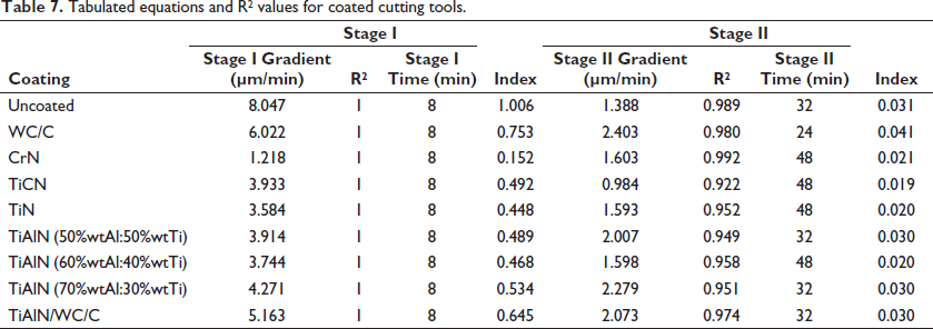
Table 7 summarizes the stages of wear for each coating. The following numbers are shown for each stage: (1) the gradient of the line of correlation, which is the wear rate of the coating for that stage; (2) the R² value, which is the amount of correlation shown for the data; (3) the machining time for that stage; and (4) the index, which is the wear rate divided by the machining time for that stage.

Table 7.

Tabulated equations and R² values for coated cutting tools.

	Stage I				Stage II
Coating	Stage I Gradient (µm/min)	R2	Stage I Time (min)	Index	Stage II Gradient (µm/min)	R2	Stage II Time (min)	Index
Uncoated	8.047	1	8	1.006	1.388	0.989	32	0.031
WC/C	6.022	1	8	0.753	2.403	0.980	24	0.041
CrN	1.218	1	8	0.152	1.603	0.992	48	0.021
TiCN	3.933	1	8	0.492	0.984	0.922	48	0.019
TiN	3.584	1	8	0.448	1.593	0.952	48	0.020
TiAlN (50%wtAl:50%wtTi)	3.914	1	8	0.489	2.007	0.949	32	0.030
TiAlN (60%wtAl:40%wtTi)	3.744	1	8	0.468	1.598	0.958	48	0.020
TiAlN (70%wtAl:30%wtTi)	4.271	1	8	0.534	2.279	0.951	32	0.030
TiAlN/WC/C	5.163	1	8	0.645	2.073	0.974	32	0.030

Tool coatings appear to have little, if any, effect on tool wear at the microscale (Figures 10 and 11). The wear characteristics for the coated tools were less than those for the coated tool with the exception that WC/C had a rapid final stage of wear (Figure 10). CrN had the lowest wear which was almost linear (Figure 8). All other coatings had rapid initial wear followed by a period of decreasing wear with increasing volume removed. As with the macroscale experimental results, ³¹ no correlations between the coating properties and wear could be detected (Table 8).

Table 8.

Summary of microscale results and coating properties.

Coating	Volume removed (mm3)	Microhardness (HV0.05)	Friction coefficient	Oxidation temperature (°C)	Mean computed temperature (°C)	Maximum computed temperature (°C)	Shear plane temperature Loewen and Shaw’’s method (°C)	Tool face temperature Loewen and Shaw’s method (°C)
CrN	41	1750	0.5	700			**	**
TiCN	41	3000	0.4	400			**	**
TiN	27	2300	0.4	600	33.53	34.53	**	**
TiAlN (60Al:40Ti)	27	3500	0.4	800	32.62	34.06	**	**
TiAlN (50Al:50Ti)	21	3300	0.3–0.35	900	32.62	34.06	**	**
TiAlN/WC/C	19	3000	0.15–0.20	800			**	**
WC/C	18	1000–2000	0.1–0.2	300			**	**
TiAlN (70Al:30Ti)	17	3300	0.4	900	32.62	34.06	**	**
Uncoated	15	1500	0.8		32.94	35.35	58.33	142

Note: *Composition of computational TiAlN is unknown; a general TiAlN coating value was computed.

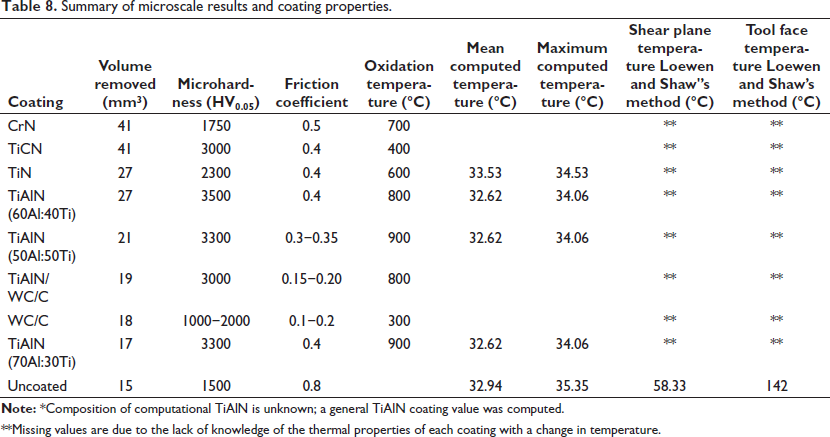
**Missing values are due to the lack of knowledge of the thermal properties of each coating with a change in temperature.

A statistical analysis was conducted on the mean volume removed at the wear criterion. A p-value less <.1 indicates that there is no significant relationship between wear and mean volume removed for a coating. Therefore, coatings do not make any difference to tool wear at the microscale. There is a slight problem using the mean volume removed rather than the maximum volume removed since the magnitude of differences are smaller. This problem is magnified at the microscale since the volume of material removed is smaller. This can be resolved by conducting one more machining experiment on another coating composition such as AlCrN, or variants, to gain an extra degree of freedom. ³¹ For all computations at the microscale, the maximum temperature was estimated 35.35°C (Table 2) and the measured temperatures for a selection of coating tools ranges between 28°C and 35°C (Table 6), which is well below the oxidation or diffusion temperature for the coating. Since validation of the computations is lacking at the microscale, pure metals with exact melting points were machined to indicate confidence in using computational results for the cutting temperature. The lowest melting point pure metal machined was potassium with a melting temperature of 64°C and there was no evidence of melting; therefore, it is highly likely that the simulations are accurate indicating that the cutting temperature is low with no heat partitioned to the workpiece. This study has shown that cutting temperatures are not high enough to accelerate tool wear. Therefore, coatings that are designed to resist wear do not exist in the high-speed micromachining regime.

An additional consideration when coating microtools is the increase in cutting edge radius, r_c, and the similarity condition known as the E-criterion. When the coating is deposited to the cutting edge of the tool, it reduces the sharpness and the concern from a coating point of view is that a chip cannot be formed (r_c >> h_cu). It has been discussed here and shown by others that in the high-speed machining regime, the feed per tooth is so small that a chip cannot be formed even with a very sharp uncoated tool (f_tooth < h_cu), and this leads to tool bending and plowing of the material. Increasing the tool edge radius with the coating exacerbates this effect but does not cause it. Therefore, the problem appears to be concerned with the initial sharpness of the microtool and the problem cannot be solved by applying successively thinner coatings as this transforms the E-criterion > 1.

The microscale cutting temperatures calculated by the Loewen and Shaw’s method ²⁸ are 58.33°C for the shear plane temperature and 142°C for the tool temperature. Although these temperatures seem realistic compared to computational and experimental results, their validity is questionable. One issue with the validity of Isakov’s formula ²⁶ is that it has never been proven in high-speed micromachining. Another problem is that the methods used to determine cutting forces are required to calculate temperatures, ²⁹ which is difficult at the microscale. Ernst and Merchant assumed that the workpiece material is perfectly plastic; ²⁹ this cannot be the case at the microscale since the tool is so small as it no longer encounters bulk material properties but individual properties of grains with variable properties (plastic and elastic), which is known as the size effect. This leads to another violation of Ernst and Merchant’s assumptions that the tool is infinitely sharp (E-criterion << 1). At the macroscale, the tool is relatively sharp and the assumption is valid. ³¹ However, at the microscale, the tool is blunt and the assumption is incorrect (r_c > h_cu). Ernst and Merchant’s method is based upon geometrical considerations and should be independent of scale.^{1, 2, 22, 29} However, when the microscale shear plane area is calculated, it turns out to be very small, which reduces the values of the normal and shear stress. As the shear plane area becomes infinitely small, the shear and normal stress become infinitely high. Therefore, at some point, the concept of the shear plane area becomes impractical and the method breaks down. That point is probably not reached in this study but would become problematic if the size of the cutting tool was reduced further. The approximation that slip plane spacing is replaced with the shear plane spacing may not be true for micromilling. The approximation is questioned further since its validation in the high-speed regime is unknown.

Another difficulty in applying Ernst and Merchant’s approach is that the uncut chip thickness, h_cu, must be known.^{27, 29} Usually, this is calculated from parameters’ set on the machine. However, the very small feed per tooth leads to bending of the tool as discussed by Kim. ⁶ The feed per tooth must accumulate to a sufficient critical value so that a chip can form; this critical value means that the uncut chip thickness is variable. ³¹ Therefore, the uncut chip thickness was estimated based on geometrical considerations (D-criterion < 1) and is one of the main limitations in accurately applying the Ernst and Merchant method. Finally, Loewen and Shaw’s method^{22, 28} to calculate the cutting temperature requires determination of the tool-chip contact length and when inspecting images of the chips, there is no evidence to suggest what this length might be. Therefore, there are many limitations in applying these calculations at the microscale.

Tool wear at the microscale does not match any of the mechanisms identified by the ISO standard 8688, ³⁰ or by Shaw. ²⁹ Rather than gradual wear of the tool flanks the entire tool tip is worn away. In addition, the stages of wear are different compared to macrotools. Only two stages of microscale wear can be identified, stage I the initial rapid stage is still present, but stage II is not steady-state, rather as the volume of material removed increases, tool wear decreases and stage III wear vanishes (Figure 13). It is probable that the lack of stage III wear is due to how the cutting tool wears away. As Figure 13 shows, the sharp cutting edge rapidly wears away in stage I since the edge is not strong enough to resist the applied cutting forces, the once sharp cutting edge is now blunt (r_c >> h_cu). At the macroscale, the tool quickly becomes rounded but is still relatively sharp and can form chips. Since a macrotool is relatively sharp, there is still an opportunity for fracture and rapid stage III wear leading to failure. ³¹ However, at the microscale, the tool becomes blunt but not relatively sharp. That means that the tool edge becomes strong but is not sharp enough for fracture of the tool to occur. The blunt cutting edge becomes so strong that it can resist large impacts when the cutter engages with the workpiece. Thus, there is no rapid stage III wear because the tool is already worn beyond the point of rapid wear. When the tool is new, the edge radius is not sharp enough to cause a chip to form (r_c >> h_cu); as previously discussed, the tool bends and eventually the uncut chip thickness becomes large enough to form a chip (r_c << h_cu). ³ As the tool becomes blunt, the edge radius increases and the uncut chip thickness must increase even further before a chip can form; the result is increased bending of the tool. This agrees with experimental observations, the longer the machining duration the more the tool bends.^{1, 2} It also explains why it is harder to wear a blunt tool than a sharp one. In summary, the microtool is too sharp to resist rapid blunting of the edges (stage I). Stage III is not present because the tool is too blunt to wear rapidly. This is also the reason why coatings appear to have little impact on the tool life since tool wear is due to the lack of mechanical strength of the cutting edge rather than by thermal effects.^{10, 11} This re-iterates the fact that microtool coatings do not need to resist high temperatures but should be designed to improve the mechanical strength of the cutting edge.

Figure 13.

Secondary flank wear due to compressive failure that caused tip wear.

As shown in Figure 1, microtools do not wear with the flank wear caused by abrasion, the entire tool tip is worn. The tool is not strong enough to resist wear and is likely to be abraded. Abrasion is caused by asperities, which gouge portions of the tool material. At the macroscale, the number of hard particles the cutting edge encounters are small and wear is low. ³¹ At the microscale, the chance of the cutting edge encountering a hard particle is even smaller. However, when it does, the consequences are more severe. ¹⁹ The cutting edge is too weak to resist abrasion by a hard particle and it fractures. The tool edge is the weakest at the tip where there is no surrounding material to support and distribute the load caused by the asperity. As a result, the area that must bear the load is small and the normal and shear stress on the tool tip is increased. Thus, the entire tool tip wears away rather than a small portion of the flank.^13–16

In contrast, the macrotool tip has more surrounding material that allows a larger area to distribute the load and the only resulting wear is flank wear.^{1, 31} At the microscale, there is some flank wear but this is a secondary function of the compressive failure that caused tip wear (Figure 13).

Owing to simultaneous wear of the tool flank and tool tip at the microscale, macroscale tool wear identification and measurement techniques are inadequate. ³⁰ In microscale milling experiments, the proposed 80 µm of flank wear criterion was converted to 80 µm of tip wear. The suitability of this criterion could be determined by investigating the tolerances of machined parts. Additionally, tip wear is not mentioned in the ISO 8688 standard, ³⁰ it is possible that tip wear could be included in that standard as either its own category or as a subcategory of flank wear. A proposed tool wear measurement using the so-called “micromilling ratio,” which is the volume of workpiece removed to the volume of tool worn away, $\mathrm{M}\mathrm{M}\mathrm{R}=\mathrm{ }\frac{{\mathrm{v}}_{\mathrm{w}\mathrm{o}\mathrm{r}\mathrm{k}\mathrm{p}\mathrm{i}\mathrm{e}\mathrm{c}\mathrm{e}}}{{\mathrm{v}}_{\mathrm{t}\mathrm{o}\mathrm{o}\mathrm{l}}}$ , would solve this problem since the wear of tool to workpiece volume removed could be identified. Essentially, MMR in micromilling is equivalent to the grinding ratio, G, in precision grinding. ³¹

Conclusions

The results of this study showed that microscale tool coatings have no effect on tool life, and that there are no correlations between the coating properties and microscale tool wear. Therefore, microscale tool wear cannot be predicted by coating properties. From the thermal viewpoint, high-speed micromilling cutting temperatures did not reach >64°C. Subsequently, thermal effects are not factors that contribute to microscale tool wear. Microscale tools wear due to the weakness of the cutting edge and that the wear criterion at the microscale is not satisfactory because wear mechanisms are different than that established for macroscale tools. In this case, the MMR ratio is quite useful. It was also discovered that the ratio of the tool edge radius to the uncut chip thickness (r_c/h_cu) required to form a chip is unknown.

The principal conclusions drawn from this study allows the authors to address problems associated with redesigning microtools and nanostructured coatings to eliminate wear, to develop standards that describe the action of microtools, and to understanding how to calculate the minimum chip thickness that guarantees the formation of chips rather than the formation of burrs.