
Abstract
Ecological momentary assessments (EMAs) and wearable devices afford opportunities to collect real-time data on events experienced in daily life. Examples of event-based data in the psychological and behavioral sciences include smoking a cigarette, experiencing a stressor, having a disruption to sleep, experiencing a depressive or manic episode, drinking an alcoholic beverage, or engaging in a bout of exercise. The increasing availability of dense sampling approaches allows for the measurement of such events at relatively fast timescales (e.g., occurring across minutes, hours, days, or weeks), expanding the possibilities for how time can be conceptualized and modeled. Survival analysis is a modeling approach that allows researchers to address scientific questions regarding whether and when events occur in time. Although not often applied to EMA data, there are myriad research questions relevant to psychosocial and behavioral scientists that can be addressed using survival analysis. In this article, we provide an overview of survival analysis, describe several time-based considerations for modeling event-based EMA data using survival analysis, and provide several illustrative examples of the different time-based considerations. Altogether, the goals of this article are to enhance knowledge of the types of research questions that can be examined using survival analysis, illustrate nuances of applying the method to EMA data, and spark ideas for future empirical and methodological research.
Keywords
Advances in mobile technologies have enabled the collection of reports about individuals’ experiences as they go about their daily lives—ecological momentary assessments (EMAs). EMA data can be conceptualized in various ways, including as events, defined as a qualitative change from one state to another at a specific time (Allison, 2014). Examples of event data include reports of stressors, social interactions, cigarette smoking, sleep onset, depressive or manic episodes, alcohol consumption, and bouts of physical activity. The increasing prevalence and frequency of daily life assessments (e.g., across minutes, hours, days, or weeks) has expanded how time can be conceptualized and modeled. Survival analysis (also known as “time-to-event analysis” and “event-history analysis”) is a family of statistical methods that addresses whether and when events occur in time. Although rarely applied to EMA data, survival analysis can answer a wide range of research questions that are relevant to psychological and behavioral scientists and align with growing calls for modeling the temporal dynamics of behavior.
Understanding when a psychological event occurs—rather than simply whether an event occurs—can help clarify points of inflection in behavior and the timescales over which relationships between “risk” factors and events unfold (Collins, 2006; Scholz, 2019; Spruijt-Metz et al., 2015). For example, knowing that increases in stress predict the highest risk of smoking within hours (rather than days) offers different insights than models that assess associations only over fixed time intervals. EMA data are uniquely suited to this purpose because they allow researchers to capture fine-grained, real-world variability in predictors and outcomes, enabling tests of how quickly a change in context or psychological state leads to a specific event (e.g., smoking lapse, onset of weekly drinking, stressor occurrence). This temporal specificity supports the refinement of psychological theories that often imply but do not test assumptions about the temporal features of psychological processes, such as latency and recurrence of behavioral responses.
In this article, we aim to demonstrate the usefulness of survival analysis for event-based EMA data and spark ideas for future empirical and methodological research. We begin with a brief overview of survival analysis and outline key time-based considerations, including examples from previous EMA studies, followed by a series of illustrative examples. Throughout, we discuss current challenges and opportunities for future research.
Survival Analysis Overview
To address scientific questions pertaining to whether and when an event occurs, a statistical model from the family of survival analysis methods can be used. Survival analysis is commonly applied to relatively long-term (e.g., months, years) longitudinal panel data in medical (e.g., disease onset or death), sociological (e.g., recidivism), educational (e.g., school graduation or dropout), and organizational (e.g., employee turnover) research (Benda, 2005; Collett, 2023; Infurna et al., 2013; Morita et al., 1989; Plank et al., 2008). Although much less common, applications of survival analysis to relatively short-term (e.g., hours, days, weeks) EMA data can be found in prior psychological and behavioral research, including examining predictors of time until smoking or abstinence, social interactions, and stressor exposure (for examples, see Table 1). Unlike traditional longitudinal panel data, EMA data afford opportunities for examining temporal dynamics on faster timescales and across multiple timescales.
Examples of Time-Based Considerations From Prior Research Using Survival Analysis to Model Event-Based EMA Data

Note: EMA = ecological momentary assessment.
Daily life data collection methods include signal-contingent (i.e., mobile prompts at fixed or random times), interval-contingent (i.e., regular prompts, daily diaries), and event-contingent (i.e., participant-initiated after a predefined event) assessments (Mehl & Conner, 2012; Myin-Germeys & Kuppens, 2022). Regardless of method, each observation includes a time stamp, enabling fine-grained temporal information on event occurrence. Throughout this article, we distinguish assessment types when relevant but otherwise use “EMA” as an umbrella term.
A variety of statistical models can be used to examine event-based EMA data, with model choice guided by the research question(s) and by particular features of the data, such as whether events are expected to occur only once or more than once. Often, the focus is on predictors of event occurrence, duration, frequency, and intensity (Singer & Willett, 2003). Most rely on longitudinal mixed models, which typically assess event occurrence or frequency but rarely assess the time it takes for events to occur. An alternative approach is to examine when events happen, defined as the time between a designated observation start point and the onset of single or recurring event (Allison, 2014).
A survival analysis is likely called for if a research question focuses on both whether and when an event occurs (Singer & Willett, 2003). Survival analysis methods (encompassing nonparametric, semiparametric, or fully parametric regression models) are the only approaches capable of accurately modeling the time to event for individuals who are at risk for but do not experience the event during the study observation period. Although survival analysis has not been featured in common textbooks on analytic methods for modeling EMA data (see e.g., Bolger & Laurenceau, 2013; Mehl & Conner, 2012; Myin-Germeys & Kuppens, 2022), there are many resources available (e.g., Allison, 2014; Elmer et al., 2025; Lougheed et al., 2019; Mills, 2010; Singer & Willett, 2003). Altogether, it is likely that this has not been a common method for modeling EMA data because of other analytic methods receiving attention in common EMA-focused textbooks, little discussion in the EMA literature on what constitutes (or could constitute) an event, and lag time in the software available for fitting survival analysis models. To bridge this gap, we provide a brief overview of the key features of survival analysis relevant in application to EMA-type data.
Two key components in survival analysis are the survival function and the hazard function. Assume that the timing in which individuals experience an event is denoted as T, which is a nonnegative continuous random variable. In continuous time, the survival function is expressed as

which indicates that the survival function at time, t, is the probability of the event time, T, exceeding t. The survival function at the earliest point in time, t0, is 1 and can only decrease as time progresses because overcoming risk and remaining event-free for longer time periods is less likely than for shorter time periods (or equally likely if there is no risk of the event during the extra follow-up). The hazard function (i.e., hazard rate) is expressed as

which indicates the instantaneous risk that an event occurs in the time interval (t, t + Δt) given that the individual was at risk to experience the event at time, t. The numerator of the hazard function is the probability that a person who has remained event-free through time

Example of (left) a survival function and (right) a cumulative hazard function for baseline models of recurring smoking episodes. (Left) The survival function (solid line) shows the probability at a person will “survive” (i.e., not experience the event) past a certain time, t. The shaded area represents the upper and lower limits of the 95% confidence interval (CI). In this example, after achieving initial 24-hr abstinence, the probability of remaining abstinent for longer than 48 hr is 0.68 (i.e., 68% of individuals who achieve initial 24-hr abstinence remain abstinent for more than another 24 hr). (Right) The sharp increase and subsequent relative plateau suggest a decreasing hazard of a smoking lapse over time. In other words, the subsequent risk for a smoking lapse markedly decreases for individuals who remain abstinent for approximately 14 days.
A frequently used model for survival analysis is the Cox regression model, which in basic form (i.e., single event with one time-invariant predictor) is expressed as

where the hazard for an individual, i, at time, t, is the product of a baseline hazard, h0(t), and the exponentiated linear function of the time-invariant predictor, xi1. There is no constant intercept term (e.g., β0) because it is absorbed into h0(t). The Cox model is also referred to as the Cox Proportional Hazards model. It is a semiparametric approach because no assumptions are made about the baseline hazard function, but it does model the association between a predictor and event with a specific functional form,
Censoring is common in time-to-event data and occurs when the timings of events are only partially observed. Right censoring occurs when the exact timing of the event is unknown for an individual, but it is known that this time to event is greater than some value. This typically occurs when an individual drops out of the study early or does not experience the event during the study period (Allison, 2014). Mathematically, if we denote
Second, the term “left censoring” has been used in different ways across the statistical and psychological literature to describe distinct scenarios. In the general context of survival analysis, left censoring refers to the scenario in which an individual’s exact time to event is unknown but it is known that it is less than some value. This can occur if a participant in the sample experiences the event before the observation period begins and cannot recall the exact date that the event occurred. This type of censoring is relatively rare and likely irrelevant to EMA studies in which events are recorded in real time and tend to frequently occur. In the psychological literature, the term “left censoring” has also been used to refer to a scenario in which the exact start of a risk period (i.e., when an individual is first at risk for an event) is unknown. Consider, for example, a study of manic episodes. If a participant starts the study in a nonmanic state, it will not be possible to precisely quantify the time until their first manic episode after entering the study because it is unknown how long the individual had been at risk for a manic episode before the participant entered the study. Thus, the period of time until the first observed manic episode is left censored because the start of the risk period is unknown. Throughout the remainder of this article, we use the term “left censoring” to refer to this latter definition. Unlike right-censored cases, left-censored cases cannot be included directly in many survival analysis methods, such as Cox regression (parametric models are an exception; Allison, 2014). However, there are data preprocessing strategies for dealing with left censoring, such as removing left-censored data before analysis (Fichman, 1989; Singer & Willett, 2003).
There is also a third type of censoring known as “interval censoring,” in which the event occurrence is observed to happen between two points in time (i.e., an interval) but precise timing of the event is unknown. Although conventional survival analysis methods are not designed to handle interval censoring directly, there are many extensions of these methods and corresponding software implementations that are available to address this issue under a similar analytical framework (Anderson-Bergman, 2017; Pan, 1999; Turnbull, 1976).
Time-Based Considerations for Applying Survival Analysis to EMA Data
EMA study designs offer diverse possibilities for generating intensive data across multiple timescales, with unique opportunities and challenges for survival analysis. Once an event of interest is identified, there are several time-based considerations with respect to the scientific research questions, data collection, data formatting, and data analysis, summarized in Table 2 and described in further detail in the following sections. Most existing studies that have applied survival analysis to EMA data quantified both event timing and predictors of event timing using EMA data. Two exceptions are studies by Steptoe and Wardle (2011) and Cleveland et al. (2023), in which the predictors were quantified using EMA data but the event timing was calculated from non-EMA data.
Time-Based Considerations for Applying Survival Analysis to Event-Based Ecological Momentary Assessment Data

Illustrative EMA study
To help illustrate the time-based considerations, we present several examples from existing research that modeled EMA data using survival analysis and use our own smoking cessation EMA study, called Prevail II (Kendzor et al., 2024), as a focal example. We conceptually describe the study in brief below and use the study data to illustrate several examples later in the article.
Prevail II participants and procedure
Brief details about Prevail II are provided below, and further details are provided elsewhere (Kendzor et al., 2024). In Prevail II, EMA data were collected using the Insight mHealth app platform. Altogether, 295 participants started the EMA portion of the study, beginning 7 days before their scheduled quit date through to 28 days post-quit date. At 10 p.m. on the night before their scheduled quit date, participants were instructed to quit smoking. The EMA procedure involved five signal-contingent EMAs per day, including a morning daily diary and four subsequent random assessments. Daily diaries contained day-level items pertaining to “yesterday” and all items contained in the random assessments that focused on momentary experiences. Participants were also instructed to initiate an event-contingent assessment if (a) they were experiencing an urge to smoke (“record an urge”), (b) they were about to smoke but had not smoked yet (“about to slip”), or (c) they had already smoked (“already slipped”). On their quit date and once per week (through Week 4 post-quit), participants visited the lab to complete additional questionnaires and provide an expired carbon monoxide reading to biochemically confirm their abstinence status.
Prevail II measures
Number of cigarettes just smoked
In participant-initiated assessments, participants were asked, “How many cigarettes did you just smoke?”; response options included 0 (I have not smoked today), 1 (between one puff and a whole cigarette), 2 (two to three cigarettes), 3 (four to five cigarettes), 4 (six to seven cigarettes), 5 (eight to nine cigarettes), and 6 (10+ cigarettes).
Time since last cigarette
In random assessments, daily diaries, and participant-initiated assessments, participants were asked, “Today, how long ago did you last smoke a cigarette?”; response options included 0 (I have not smoked today, not even a puff), 1 (0–15 min ago), 2 (16–30 min ago), 3 (31–60 min ago), 4 (61–120 min ago), 5 (121–240 min ago), 6 (241–480 min ago), and 7 (over 480 min ago).
Cigarettes smoked yesterday
In daily diaries, participants were asked, “How many cigarettes did you smoke yesterday?”; response options included 0 (I did not smoke yesterday), 1 (between one puff and a whole cigarette), 2 (two to five cigarettes), 3 (six to 10 cigarettes), 4 (11–15 cigarettes), 5 (16–20 cigarettes), 6 (21–25 cigarettes), and 7 (25+ cigarettes).
Cumulative day-level smoking status
In random assessments, daily diaries, and participant-initiated assessments (record an urge), participants were asked, “Today, have you smoked any cigarettes (even a puff)?”; response options included 0 = no and 1 = yes.
Affect
In each daily diary, random assessment, and participant-initiated assessment, participants were asked about their momentary positive and negative emotions: “I feel [happy, calm, irritable, frustrated/angry, sad, worried, miserable, restless, bored, depressed, anxious].” Responses were provided using a 5-point Likert scale ranging from 1 (strongly disagree) to 5 (strongly agree). Positive affect at each assessment was calculated as the average of the two responses to relevant items. Negative affect at each assessment was calculated as the average of the nine responses to relevant items.
Visualizing abstinence episodes and smoking events
Figure 2 depicts four prototypical participants who we repeatedly refer to in the following sections to illustrate several of the time-based considerations. In brief, the bottom row of Figure 2 depicts whether the participant started the post-quit period in a state of smoking. Participants who did not establish 24-hr abstinence on their scheduled quit date have a gray rectangle depicting how many days it took to establish initial 24-hr abstinence (e.g., 8 days for Participant 2). The second row (dark blue rectangle) depicts number of abstinence days that occurred while the participant was at risk for the first post-quit smoking lapse. Participants who had an initial smoking event are marked by the transition from a dark blue rectangle to a gray rectangle. Gray rectangles show how many days each smoking event lasted and represent days not at risk for a smoking event because the participant is still in a current smoking event. Participants who had an initial smoking event but reestablished 24-hr abstinence are marked by a royal-blue rectangle in the third row from the bottom. If a participant ended the study period because of either the study ending (e.g., Participant 1) or dropping out of the study early (e.g., Participant 2) in a given episode while in a state of abstinence, it is denoted by a coral diamond (i.e., they are right censored). Participant 3 does not have a coral diamond at the end of their second episode; instead, Participant 3 has a gray rectangle, which indicates they ended the study period in a state of smoking.

Time until smoking events for recurring abstinence episodes. Segments that are shaded with distinct colors represent distinct periods of initial or recurring abstinence, whereas segments that are shaded in gray represent periods of smoking. If there is a gray bar before the first abstinence episode, it indicates that smoking occurred during the quit date before establishing initial 24-hr abstinence. A gray bar to the right of an abstinence episode indicates a smoking lapse. Coral diamonds indicate right censoring.
Time-based considerations for defining events
Event timing can be quantified using one or more EMA data types (Mehl & Conner, 2012; Myin-Germeys & Kuppens, 2022). The following sections describe several time-based considerations for defining events when constructing a survival analysis model.
Defining the start of the event risk period
Quantifying time to event(s) requires defining when individuals are “at risk,” meaning they are in a state in which the event could occur but has not yet happened. For example, establishing 24-hr abstinence might mark the start of the event risk period for a smoking lapse. Likewise, the first peak-sadness report has been used to mark the start of the risk period for consuming alcohol (Hussong, 2007). The start of the event risk period does not always correspond to the start of the study. In smoking cessation research, observation may begin at the target quit date, but the risk period starts at the first 24-hr abstinence, when lapse becomes possible. For some, this abstinence period coincides with the quit date (e.g., Participants 1 and 3 in Fig. 2); for others, it occurs days later (e.g., Participants 2 and 4 in Fig. 2, shown by the bottom gray rectangle not aligned with an episode).
An approach for handling mismatched risk periods and observation intervals involves removing initial data from a participant’s time series in which they are not yet at risk for the event. This aligns all participants’ time series to a common baseline when it is first possible for the event to occur (Fichman, 1989; Singer & Willett, 2003). Returning to the smoking lapse event example, this would mean excluding any assessments before each individual’s initial 24-hr abstinence if they did not quit immediately on the individual’s target quit date. Similarly, Elmer et al. (2025) excluded the first social interaction of each day when examining affect and time to subsequent social interactions, defining the daily risk period to begin at the end of the first social interaction.
Defining the unit of time
The defined unit of time (e.g., minutes, hours, days) should align as closely as possible to the smallest unit relevant to the process being studied (Singer & Willett, 2003). Conversions between units of time (e.g., hours to minutes) change only the interpretation of the analysis and not the analytical approach or results as long as the conversions maintain the same level of precision. In the studies that applied survival analysis to EMA data, the most common time unit was days; other time units included minutes, hours, weeks, or years (for specific study details, see Table 1). The time unit can also be defined with respect to the study design, for example, as the number of exposures to EMA prompts until a participant drops out from the study (Murray et al., 2023). In this case, a discrete-time-hazard model may be more appropriate than continuous-time methods because the number of exposures can take only integer values (Kalbfleisch & Prentice, 2002).
A key consideration is whether certain times should be excluded from the EMA data, such as nighttime periods when participants are typically asleep and therefore not providing EMA data. Some studies exclude these periods. For example, Elmer et al. (2025) removed overnight intervals when examining whether affect during social interactions was associated with time until the next interaction. They excluded the first interaction of each day, which assumed each day’s affect started fresh. In contrast, other behaviors, such as smoking or drinking, can occur at any hour, so EMA studies on substance often include both random signal-contingent and participant-initiated event-contingent assessments. In studies in which random assessments are limited to waking hours, event-contingent assessments are often the only way to capture events that occur during typical sleep times.
Another consideration is the expected number of ties, instances in which multiple individuals share the same event time (e.g., two people lapse 3 days after initial abstinence). The prevalence of ties is one source of information that can be used to inform whether to use a discrete or continuous time-survival analysis. Given the temporal precision of EMAs, continuous-time methods, such as Cox regression, are often feasible, even with integer-valued time-to-event data and ties (for more information on discrete- vs. continuous-time methods, see e.g., Allison, 2014; Mills, 2010; Singer & Willett, 2003). However, when ties are frequent—such as when time is measured more coarsely than the event rate (e.g., alcohol use tracked weekly)—continuous-time methods are less suitable because a continuous random variable should theoretically not have ties. When ties occur, methods such as the Efron approximation can be used during model estimation (Efron, 1977), but if ties outnumber unique event times, discrete-time models may be more suitable (Chalita et al., 2002; Singer & Willett, 2003). Using continuous-time models with many ties can bias coefficients toward zero (Mills, 2010). Note that few EMA-based studies have reported the number of ties or how the extent of ties informed modeling choices.
Defining the event start
The event start marks the point when a person transitions from the absence to presence of an event. This can occur at a specific moment, such as the first puff of a cigarette (Kirchner et al., 2012). This transition can also be conditional on a time-based threshold, such as initial smoking abstinence defined as 24 hr without a cigarette (Piper et al., 2020). Event onset can also depend on the accumulation of behaviors, such as binge drinking, defined by consuming four plus drinks for women or five plus drinks for men in 2 hr (National Institute on Alcohol Abuse and Alcoholism, 2024; Wechsler & Nelson, 2001). In this example, the event onset is also conditional on a person-level characteristic (i.e., gender). Accuracy of the event start is tied to the EMA design. One way to improve accuracy is to include items asking about whether an event occurred and if so, how long ago to get a more precise measure of event occurrence and timing. Another option is to use a combination of random and participant-initiated assessments. This is beneficial when the random assessments are confined to participants’ wake times, allowing for participant-initiated assessments to capture events outside typical wake times. Daily diaries can help catch missed events from the previous day, including those that happen after the last random assessment and in times when participants forget to initiate their own assessments or fail to answer any of the prior-day random assessments.
Event status and right censoring
When estimating a survival model, the time-to-event outcome (or maximum observed time) is specified along with an event indicator for the risk period (0 = event did not occur, 1 = event occurred). Right censoring occurs when an event is not observed for an individual during the study period. These individuals may or may not experience the event after the study is over. In a recurring events model, it is also possible that some individuals will experience the event several times but that their last episode will be right censored. Figure 2 shows several illustrations of event status and right censoring. Participant 3 ended the study period while smoking (the event of interest) and thus is not right censored, denoted by no coral diamond at the end of their second abstinence episode. Participant 4 has six abstinence episodes, each marked by a colored horizontal bar. The first five episodes ended with a smoking event, whereas the sixth episode is right censored because the study period ended (denoted by a coral diamond at the end of the top bar).
Right censoring is informative if it is associated with the event (e.g., a participant drops out of a smoking cessation study because they resumed smoking but did not report this to the research team) and noninformative if it is independent of the event (e.g., the research study period ends or a participant drops out of the study early because they moved away). Participant 2 was right censored before the study ended, potentially in an informative way. In contrast, Participant 1 was likely noninformatively censored because of the study’s end. Some events, such as intervention efficacy, may have higher rates of informative right censoring compared with everyday events, such as social interactions. Informative censoring is especially problematic when the reasons for dropout related to the event are unmeasured. In contrast, if dropout is associated with a measured variable (e.g., men dropping out earlier than women), it can be accounted for in the survival analysis. For example, Cox regression will still provide unbiased estimates if the measured variables associated with censoring are included as predictors in the model. In other types of survival analyses that depend on the marginal distribution of underlying survival times, inverse-probability of censoring weights may be constructed based on the measured variables, which can then be used to emphasize the datapoints from the sample that were less likely to be observed because of right censoring. This general weighting approach allows one to eliminate the influence of right censoring and construct an analysis that is more representative of the target population, assuming the weights are correctly specified (Gerds et al., 2013; Kalbfleisch & Prentice, 2002; Willems et al., 2018).
Defining the event end
Events can span across one or more EMAs, which relates to how the end of an event is defined. In some cases, the event start and event end are captured by a single EMA, such as when a smoking lapse is defined as both the first puff and the last cigarette reported in the same EMA (Kirchner et al., 2012; Shiffman et al., 1996). In other cases, the event may span across several EMAs, such as when the end of a lapse is defined as the moment just before reestablishing 24-hr abstinence, spanning across multiple EMAs. When an event can occur more than once, precision in defining the end of the event is important so that it is clear when someone becomes at risk for the next event to occur.
Defining the number of times an event can occur
The number of times an event can occur affects the data preprocessing and choice of survival model. For events that can occur only once (e.g., initial 24-hr abstinence), a single event survival model should be fit to the data. In a recurring events model (e.g., recurring smoking events), each event occurrence is part of an episode, which is defined as the time between when someone is first at risk for an event (either first occurrence or recurrence) up until the onset of the event. Recurring event models often include a frailty term, similar to a random intercept in multilevel models, which modifies the hazard function to account for between-person differences in risk for the event (Lancaster, 1979; Mills, 2010; Vaupel et al., 1979). For example, some individuals may naturally be more susceptible to a recurring event, resulting in many short time intervals in between the events. Frailty terms account for this variation in susceptibility and the correlation that it induces between interevent times from the same subject. These frailty models are often specified under a proportional hazard framework (similar to the Cox model for single event outcomes in Equation 3), such as

where, hij(t) is the hazard function for individual, i, and event occurrence, j, at time t; h0(t) is the baseline hazard function; exp(νi) is the random frailty term that accounts for the correlation between interevent times from the same individual; and exp(β1xij) is the time-fixed term that reflects the multiplicative effects of each predictor, xij, on the hazard function. It is often assumed that the frailty term follows a gamma distribution, but other distributional assumptions, such as the lognormal model, are possible (Aalen, 1988; Hougaard, 2000; Mills, 2010).
Defining times when event risk cannot be determined
Ideally, EMA sampling is frequent enough to capture events accurately, and participant-initiated assessments can also help ensure event detection. However, missing data pose challenges. When quantifying event timing and determining a strategy for handling missing data, it is useful to consider the length of time between two observed EMAs and whether the event was reported to occur in the EMAs on either side of a period of missingness. For example, in a study with random assessments spaced 3 hr apart, missing one EMA might not introduce much uncertainty, but missing six EMAs makes it more difficult to accurately calculate time to an event. Ideally, before formatting data for survival analysis, a plan is determined for how much time can elapse before there is too much uncertainty about whether the event occurred during the period of missing data.
Decisions about how to handle missing data for survival analysis can also depend on whether the event was occurring before and/or after the period of missingness. For instance, consider a participant who reports abstinence before and after a day of missed EMAs. It is possible the participant remained abstinent but also possible that they had a smoking event, which may or may not relate to why they skipped the EMA (recall discussion of informative right censoring above). In contrast, there are certain times when missing data may not be problematic. Consider a participant who reported smoking (the event of interest) before and after a period of missing EMAs. In this scenario, missing data do not affect event timing because the participant was not currently at risk to experience the event (i.e., if the next risk period begins only when 24-hr abstinence is reestablished).
When EMAs are missed, there are strategies that can be considered before data analysis. Few existing studies that applied survival analysis to EMA data explicitly discussed how missing data were handled in the calculation of event times. Of the studies with these details, methods included removing the episode altogether (Armeli et al., 2008; Hussong, 2007), marking the episode as right censored on the first occasion with missing data (Armeli et al., 2008), and including missing days in the calculation of the time to the next event occurrence (i.e., assuming the event did not occur on days with missing data; Armeli et al., 2008; Lougheed et al., 2023) Armeli et al. (2008) conducted sensitivity analyses and found that their results were substantively similar for each approach. In the broader literature on time-to-event models, there are several approaches to missing data, including (a) removing the episode altogether, (b) carrying the last observation forward, (c) assuming the event occurred, (d) censoring the episode, and (e) using a model-based imputation procedure. Some approaches are better than others for handling missing data in terms of the caveats or assumptions that are made (see e.g., Lachin, 2016; Little & Rubin, 1983).
Time-based considerations for defining predictors
There are also time-based considerations for defining predictor variables in survival analysis models. Some research questions may correspond to predictors that are time-invariant or fixed (e.g., intervention group assignment), whereas other predictors may be time-varying (e.g., day-to-day variation in positive affect).
Time-based predictors related to event occurrence
There are several approaches for including time-based predictors of event occurrence that can serve to address scientific research questions or as covariates/control variables. One approach is to include historical indicators of the event, such as the number of suicide attempts before entering the research study (Porras-Segovia et al., 2023). A second approach is to include a predictor corresponding to event exposure during the study. For example, Elmer et al. (2025) used the number of social interactions in the past 24 hr to predict the next social interaction. Event sequence number can also be used to examine whether progression through events predicts future event risk (i.e., linearly or curvilinearly; Kirchner et al., 2012). The event sequence number can also be specified as a strata variable (instead of a predictor variable) in a recurring events model, which modifies the baseline hazard for each episode. However, the stratified Cox model may not be appropriate if it is expected that the association between predictors and the hazard differ across strata (i.e., an interaction between the predictor variable and the strata variable) and/or if there are specific research questions on how event sequence is associated with risk of each recurring event (Singer & Willett, 2003). When the first event is of particular interest, a dummy variable can indicate its occurrence. Including a shared frailty term is critical to control for heterogeneity in event susceptibility, which can otherwise lead to spurious effects of event sequence (Allison, 2014). For instance, participants with many prior lapses may be naturally prone to lapse quickly again independent of prior lapses. A third approach is to model the duration of a previous event as a predictor of time to the next event. For example, Epler et al. (2014) examined whether the duration of a period of drinking was associated with timing of the next drinking event, and Kirchner et al. (2012) assessed whether abstinence duration predicted time to the next smoking lapse.
Timescale of predictors
Predictors of event timing can operate on various timescales, with previous examples including features of time itself. One approach is to examine whether event timing differs by time of day. For example, one study found social interaction events occurred sooner when it was daytime (1 = between 7 a.m. and 6 p.m.) compared with other times (0 = all other times; Elmer et al., 2025). Other possibilities include day of week (Armeli et al., 2008; Epler et al., 2014) and social calendar. The social calendar has been operationalized as a binary variable with categories for weekend and weekday and by the proximity of a given day to the weekend (i.e., days before weekend onset; Hussong, 2007). This allows for addressing research questions on whether events are expected to occur sooner versus later as the proximity to the weekend decreases. A fourth possibility is to examine whether timing of events differs by historical period (e.g., before/during/after COVID-19; Lougheed et al., 2023).
EMAs collected over a specific period might also be used to calculate person-level dynamic characteristics (Ram & Gerstorf, 2009). For example, Chandra et al. (2007) used data from 16 days before a smoking quit date to identify prequit smoking patterns, which were used to predict time to smoking abstinence, first lapse, and relapse. Other studies calculated person-specific slopes across multiple EMAs. For example, Cleveland et al. (2023) calculated coupling between negative affect and craving across 12 days during residential treatment and found that individuals with weaker coupling tended to experience quicker posttreatment relapse than individuals with stronger coupling. Likewise, Vinci et al. (2017) calculated each participant’s positive emotion trajectory from a smoking quit date to the individual’s first post-quit smoking lapse. For each participant on each day between target quit date and first lapse, they extracted values for the slope and examined whether these values were associated with the risk of next-day smoking lapse. When including time-varying predictors, using lagged predictors is useful for minimizing inference problems because of rate and state dependence (Singer & Willett, 2003). A joint modeling approach can also be considered when there are research questions pertaining to how time-varying predictors are associated with the timing of events (Abbott, Dempsey, et al., 2024; Abbott, Nahum-Shani, et al., 2024). Joint modeling accounts for measurement error in the covariates by simultaneously modeling longitudinal changes in the true covariate values, whereas conventional survival models assume observed covariate values are measured without error. In addition, joint models can be especially useful for modeling time-varying covariates that depend on the underlying risk or occurrence of the event (known as “internal” or “endogenous” covariates; Rizopoulos, 2012).
Illustrative Examples
The following examples use Prevail II data to illustrate a selection of the time-based considerations. The illustrative examples build on examples in existing survival-analysis textbooks (Singer & Willett, 2003), including those with R code (Andersen & Ravn, 2023; Kleinbaum & Klein, 2012; Mills, 2010), and review articles (Elmer et al., 2025; Lougheed et al., 2019). All models were fit using R (Versions 4.3.1 and 4.5.0), RStudio, and the survival package (Posit Team, 2023; R Core Team, 2023; Therneau, 2023). Descriptives were calculated using the Psych package, and visualizations were created using ggplot2 (Revelle, 2023; Wickham, 2011).
Disclosures
Data preprocessing, analysis, and visualization code are available on OSF (https://osf.io/shja8/). Because the Prevail II data are not open source, we provide simulated data and code that illustrate several data formatting and analysis steps.
Prevail II descriptives
Of the 295 participants who started the EMA period 7 days before their scheduled quit date, 272 participants provided data for one or more post-quit phase EMAs, which spanned 28 days. On average, participants responded to either EMA prompts or self-initiated EMAs on 23.3 post-quit days (SD = 8, minimum = 1, maximum = 28), including 19.6 daily diary assessments (SD = 8.1, minimum = 1, maximum = 28) and 78.3 random assessments (SD = 33.4, minimum = 1, maximum = 112). In addition, 57.1% of participants self-initiated at least one smoking-urge, about-to-lapse, or already-lapsed assessment (M = 13.5, SD = 25.0, minimum = 1, maximum = 202). Similarly, on average, participants completed 4.3 assessments (SD = 9.3, minimum = 1, maximum = 66) that were sent as a follow-up to a subset of the participant-initiated assessments. Across participants, 271 responded to at least one smoking-related EMA, and smoking was reported on 37% of EMAs (SD = 26%, minimum = 0%, maximum = 100%).
Prevail II initial data processing
We combined information across each smoking variable described above to obtain more accurate time stamps for when individuals smoked. For example, instead of relying on the random-assessment time stamps, we subtracted the reported time since last cigarette from EMA time stamps to get a more accurate account of when smoking occurred. Days with missing data required special consideration because there are several potential reasons for the missing data. One possibility is that individuals did not self-report a smoking lapse and the reason for missing data for a given day had to do with reasons entirely separate from smoking. Another possibility is that a person smoked and forgot to initiate an event-contingent assessment and/or that the reason why a day had all missing EMAs and no event-contingent reports is because the person had lapsed but did not want to report it. To capture each of these possibilities, we used two different methods for handling days with no information about smoking. First, we used a last observation carried forward approach (termed nalocf ); if someone was abstinent on a given day and missing data on the next day, we marked the day as an abstinence day (this aligns with the first possibility given above). Second, we used a more conservative approach in which days with fully missing smoking data were assumed to be a smoking day (termed na1; this aligns with the second possibility given above). Next, we recast the irregularly spaced time series data into an hourly data frame such that each person had a record for each hour between the first observed study day during the EMA period and the last observed study day during the EMA period. Hourly records without an observed time stamp for smoking status were filled in using a last observation carried forward approach. Given that it is impossible to know the true reason for why data were missing for a given participant on a given day, we propose these two methods and illustrate how they can be used as a sensitivity check of the robustness of the results below in Illustrative Example 2. Future researchers might also consider the use of the methods based on the nuances of their data.
Illustrative Example 1: defining the start of the event risk period
Data preprocessing
In this illustrative example, we examine different ways to define the start of the event risk period during the post-quit phase in Prevail II. Participants were instructed to quit smoking by 10 p.m. on Day 6, with Day 7 intended as the first full day of smoking abstinence. Some participants (n = 11) had an EMA between 10 p.m. and 11:59 p.m. on Day 6. We specified three options for defining the start of the event risk period: (Definition 1) starting at 10 p.m. on Day 6 using the last observation carried forward from earlier in the day, (Definition 2) starting at 10 p.m. on Day 6 and assuming abstinence for the 10 p.m. and 11 p.m. intervals unless smoking was reported, or (Definition 3) starting with the first observed EMA after 10 p.m. on Day 6. The focal time-based considerations include defining the start of the event risk period and defining event status and right censoring.
Descriptives
Beginning at 10 p.m. on Day 6, the average time until the next observed EMA was 10.7 hr (SD = 3.1) across the 96% (n = 260) of participants who responded to one or more EMAs on their target quit date. For the remaining participants (n = 11), the first EMA occurred 160.3 hr (SD = 82.1) into the post-quit period. Several differences were observed based on the event risk period start definition (Table 3). First, there were differing numbers of participants who immediately established initial 24-hr abstinence (nOption1 = 38; nOption2 = 104; nOption3 = 105). Implications of the different definitions pertain to the sample size of participants who would be eligible to be included in a hypothetical subsequent survival analysis examining predictors of the time until initial 24-hr abstinence. Specifically, individuals who immediately establish initial 24-hour abstinence would not be eligible to be included in the analysis, and thus, the analysis would include fewer participants if Definitions 2 or 3 were used. Second, there were differing numbers of right-censored participants (Table 3, Column 4) who would be eligible to be included in the hypothetical subsequent survival analysis. The majority of the right censoring was due to the observation period ending at Day 34 (nOption1 = 56.5%, nOption2 = 56.5%, nOption3: n = 66.0%). The remaining right-censored participants dropped out before the end of the EMA period, with the potential for informative right censoring in cases when dropout occurs because of establishing abstinence. This seems unlikely, though, given that the Prevail II participants were paid for cumulative abstinence. Third, there were differences in the number of individuals who established 24-hr abstinence during the study period and in the median time until they established initial 24-hr abstinence (Table 3, Column 3). Fourth, the maximum number of ties (which influences precision of the estimated regression coefficients; Mills, 2010) for a given event time differed between the three options (Table 3, Column 7).
Descriptive Statistics Based on Different Definitions of the Beginning of the Event Risk Period

Illustrative Example 2: previous event duration and risk of a subsequent event
The primary goal for this example is to illustrate a recurring event survival model with a time-based predictor related to event occurrence that varies over time but has only one score per episode. The focal time-based considerations include (a) defining the number of times an event can occur, (b) defining times when event risk cannot be determined, and (c) time-based predictors related to event occurrence. Specifically, we examine whether the duration of the previous smoking lapse is associated with risk of the next lapse. In addition, we conduct a sensitivity analysis to examine whether results differed based on the method for handling missing smoking data, which we term nalocf and na1.
Data preprocessing
For illustration, we define the beginning of the event risk period as the first hour in which 24-hr abstinence is reestablished after each post-quit lapse. We included participants who established initial 24-hr abstinence during the post-quit period (n nalocf = 218; n na1 = 211) and excluded those who did not (n nalocf = 53; n na1 = 60). We also excluded participants who did not reestablish abstinence after at least one lapse (n nalocf = 97; n na1 = 79) because we could not calculate the duration from start to finish of a prior lapse. These criteria yielded analytic sample sizes of 121 participants (nalocf method) and 132 participants (na1 method). Next, we preprocessed the data into a person-period format, which included one row for each abstinence episode (i.e., each time 24-hr abstinence from smoking was established after a smoking lapse). For each episode, we calculated (a) how many hours elapsed from the time of establishing 24-hr abstinence until the time that any smoking occurred, or the time until the participant either dropped out of the study or the study period ended; (b) whether smoking was observed for that episode; and (c) the duration in hours for the prior smoking lapse.
Descriptives
To illustrate the types of descriptives that may be useful to report, we present descriptives based on the nalocf method and show descriptives for both methods in Table 4. During the post-quit period, the median number of smoking events was 2, the median number of hours of abstinence before each smoking event was 60, and the median duration of each smoking lapse was 32 hr. Altogether, 63 participants were right censored at the end of the EMA period, with 24 participants fully right censored (i.e., once they reestablished abstinence after the first lapse, they did not smoke again). Of the right-censored participants, 88.9% (n = 56) made it to the end of the EMA period. The seven participants who discontinued participation in the EMAs are potentially cases with informative right censoring. In this example, informative right censoring is plausible if a participant discontinued the study because the participant resumed smoking. In contrast, informative right censoring would not be the case if the participant discontinued the study early because the EMA protocol was too burdensome.
Descriptive Statistics Based on Different Methods for Handling Missing Smoking Event Data

Model
To examine whether the duration of the previous smoking lapse before reestablishing 24-hr abstinence is associated with risk for a subsequent lapse, we followed the recurring event framework described in the Defining the Number of Times an Event Can Occur section and Equation 4 above and fit the following model:

where the hazard of transitioning from abstinence to smoking in episode, j, for participant, i, hij(t), is a product of the baseline hazard function, h0(t), an exponentiated participant-specific random effect, vi, that indicates the extent to which participants differed in their risk for smoking, and the exponentiated linear function, where β1 allows for examining whether the hazard of transitioning from abstinence to smoking differs based on the duration of the previous lapse, DurationPreviousLapsei,j-1. We assumed the frailty followed a gamma distribution. More details on frailty distributions can be found elsewhere (Aalen, 1988; Hougaard, 2000; Mills, 2010).
Results
To ease interpretation of the coefficients, we rescaled the DurationPreviousLapsei,j-1 scores by dividing by 24 to correspond to days. Additionally, reported parameter estimates are transformed into the hazard ratio metric (i.e., HR = exp(β)). The HR represents the multiplicative change in the event rate associated with a one-unit increase in the predictor. An HR > 1 indicates that higher values of the predictor are associated with a higher instantaneous risk of the event, an HR < than 1 indicates a lower risk, assuming proportional hazards, and an HR = 1 indicates no association between the predictor and outcome. The results indicated a positive association between the duration of the previous smoking lapse and risk for a subsequent lapse (HR = 1.051, 95% confidence interval (CI) = [1.003, 1.102]). Specifically, for every additional 24-hr increase in duration of the previous smoking lapse, the risk of the next smoking lapse was expected to increase by 5.1% (percentage change = 100 × (1.051 – 1) = 5.1). Figure 3 shows survival curves for the 25th percentile (0.5 days; yellow dashed line) and the 75th percentile (3 days; blue solid line) of the DurationPreviousLapse predictor. The frailty variance, vi, was estimated to be 0.51. The frailty can be interpreted by exponentiating the standard deviation, exp(0.71) = 2.03. This indicates that a participant who is +1 SD above the mean on risk of smoking lapse has 2.03 times the risk of lapsing than a participant with average risk.
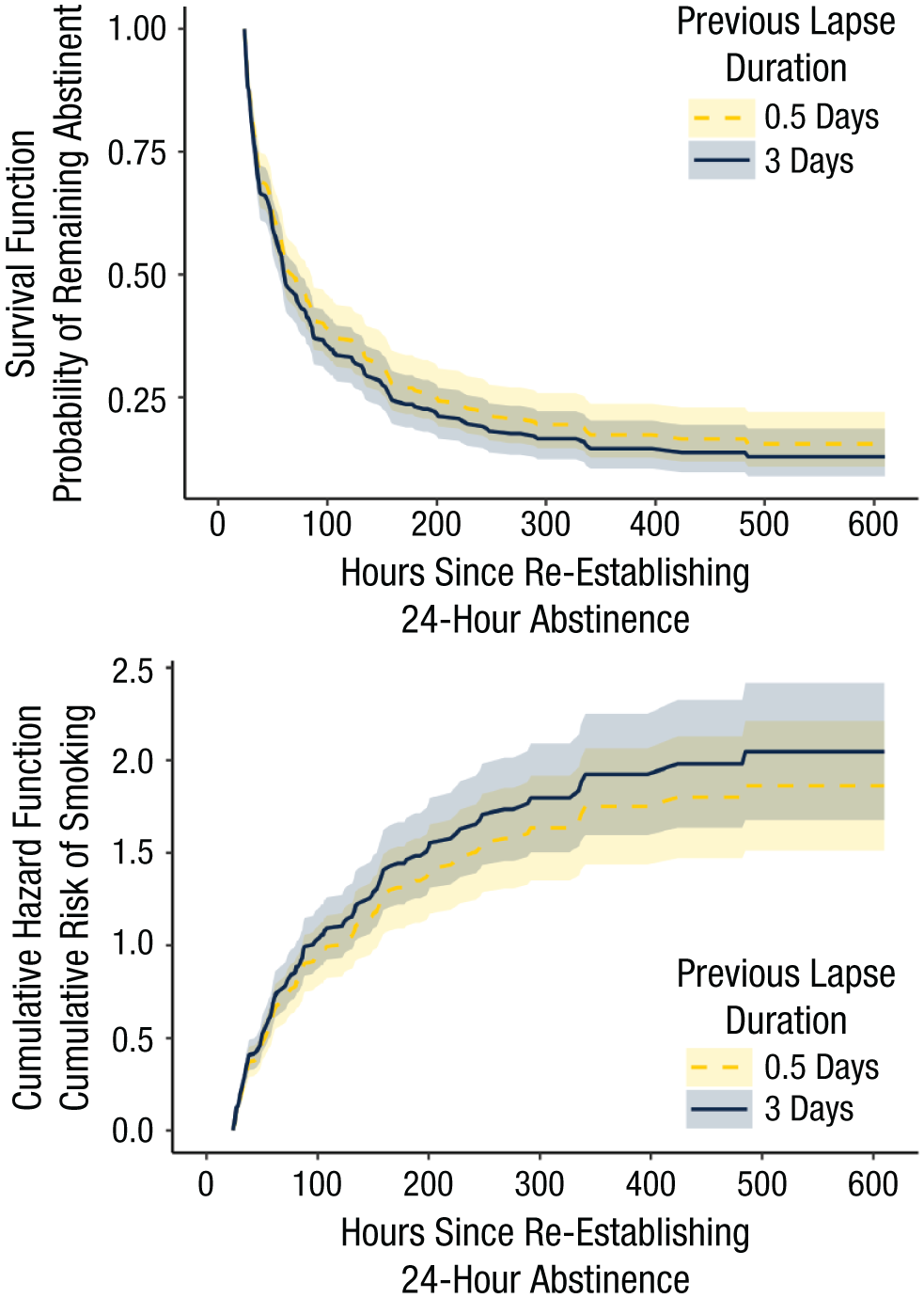
(Top) Survival functions and (bottom) cumulative hazard functions for different levels of previous lapse duration (i.e., 0.5 days, 3 days).
Next, we conducted a sensitivity analysis to examine whether the results changed based on how missing data were handled. Specifically, we refit the model using a more conservative approach assuming smoking for days with fully missing data (rather than last observation carried forward, as was used in the main analysis for this section; for more details on each approach, see Prevail II Initial Data Processing section). The results showed the association between duration of the previous lapse and risk of the next smoking event was not statistically significant (HR = 1.047, 95% CI = [0.997, 1.098]) even though the point estimates for the hazard ratios were similar across both models.
Illustrative Example 3: lagged time-varying predictors of event risk
In this example, we illustrate a lagged time-based predictor with multiple instances per episode. The focal time-based considerations include (a) defining the unit of time and (b) timescale of predictors. We examined whether prior-day positive and negative affect were associated with the risk of current-day smoking. We used the lagged affect scores so that there would be clear temporal ordering between the affect experiences and smoking events. Unlike the previous examples, the time unit was specified as days rather than hours. This was because emotions were assessed up to five times daily but no additional data on the timing or duration of emotions were available.
Data preprocessing
Participants were excluded if they did not establish initial abstinence, defined as 1 full calendar day (n = 63), and if all scores for positive and negative affect were missing (n = 4). The analytic sample consisted of 204 participants. The event risk period start corresponds to the first post-quit calendar day when a full day of abstinence is observed for the first episode and the first post-quit calendar day in which a full day of abstinence is reestablished after a lapse for all subsequent episodes. For each day in each episode, we calculated (a) a start variable, which equals zero at the beginning of each episode and increases by 1 for each subsequent day of abstinence in the episode; (b) a stop variable, which has a value of 1 at the beginning of each episode and increases by 1 for each subsequent day of abstinence in the episode; (c) a smoking status variable indicating whether smoking occurred (= 1) or not (= 0) each day; (d) the intraindividual mean (iMean) of positive affect scores from the prior day; and (e) the iMean of negative affect scores from the prior day.
Descriptives
As part of formatting these data for survival analysis, we removed any days from the time of the quit date through the time when the participant established a full calendar day of abstinence. Most participants (51.5%) achieved abstinence on their target quit date and thus had zero of these days without risk. For the remaining participants, the number of days it took to achieve abstinence after the target quit date ranged from 1 to 27 (Median = 4). The median number of abstinence episodes was 1 (M = 1.9, minimum = 1, maximum = 6). During the EMA period, 75 participants (36.8%) never had a smoking event, and 129 participants (63.2%) had at least one smoking event (M = 1.9, SD = 1.1, minimum = 1, maximum = 5). Altogether, 133 participants were right censored at the end of the EMA period (i.e., remained abstinent). Of the right-censored participants, 75 (36.8%) were fully right censored such that once they established initial 24-hr abstinence, they did not report smoking in any EMA. The majority of the right censoring was due to the observation period ending at Day 34 (n = 113, 85.0%). This left 20 participants (15.0%) who dropped out of the EMA portion of the study before Day 34 and therefore are potentially cases of informative right censoring if their dropout occurred because of resuming regular smoking unbeknownst to the research team. For episode-specific days (i.e., including only abstinence days when someone was at risk for a smoking event and excluding days when individuals were in the midst of smoking), rates of missing data were relatively low for positive and negative affect (M = 0.9 days, SD = 1.9). The average prior-day iMean for positive affect was 3.4 (SD = 0.7) and was 2.3 (SD = 0.8) for negative affect. Before model fitting, we rescaled affect iMean scores by subtracting 1.
Model
To examine whether previous day affect was associated with the risk of current day smoking, we fit the following model:

where the hazard of transitioning from abstinence to smoking in episode, j, for participant, i, hij(t), is a product of the baseline hazard function, h0(t), an exponentiated participant-specific random effect, vi, that indicates the extent to which participants differ in their risk for smoking, and the exponentiated linear function, where β1 allows for examining whether the hazard of a smoking lapse differs based on affect observed on the previous day, Affectij(t – 1). We assumed the frailty followed a gamma distribution. The model was fit separately for positive affect and negative affect.
Results
Positive affect was not associated with the hazard of a smoking lapse on the next day (HR = 0.9, 95% CI = [0.7, 1.1]). There was a positive association between negative affect and risk of a smoking lapse the next day (HR = 1.4, 95% CI = [1.01, 1.7]). Specifically, for every unit increase in negative affect, the risk of smoking the next day was expected to increase by 40% (percentage change = 100 × (1.4 – 1) = 40). For both models, the standard deviation of the frailty, vi, was estimated as 0.96. Exponentiating the standard deviation of the frailty (exp(0.96) = 2.61) indicates that a participant who is +1 SD above the sample mean on risk of smoking lapse has 2.61 times the risk of lapsing than a participant with average risk.
Discussion
The goal for this article was to enhance knowledge of how survival analysis is a useful, underused method for modeling event-based EMA data. To facilitate future research, we described several time-based considerations for developing research questions and conducting survival analysis using psychological and behavioral event-based EMA data. These included defining the beginning of the event risk period, defining the unit of time, defining the event start, examining right censoring, defining the event end, defining the number of times an event can occur, and defining times when risk for an event cannot be determined. As part of this, we drew on existing empirical research applying survival analysis to EMA data and also presented our own illustrative examples using EMA data from the Prevail II smoking cessation intervention study. Throughout, we discussed several challenges and opportunities for future empirical and methodological research.
In this article, we illustrate how survival analysis, when applied to event-based EMA data, can advance psychological theory by making time an explicit, testable dimension of behavior. Many theories imply that internal states, such as craving, affect, and motives, dynamically increase the probability of an event—such as a smoking lapse or a stressor—but do not specify how quickly these changes translate into event onset. Survival models fill this gap by modeling latency: that is, they reveal not just if a person is at higher risk but also changes over time in risk. For example, Kirchner et al. (2012) used survival analysis as a novel test of the abstinence violation effect, predicting that stronger abstinence-violation effects after a lapse would lead to faster progression from a lapse to a full relapse (Marlatt & Gordon, 1985). Similarly, Armeli et al. (2008) used survival analysis to test processes related to self-regulation, predicting that increases in mood early in the week would lead to faster drinking within the weekly cycle (i.e., immediacy). In these studies and others, EMA enabled this level of temporal precision by capturing time-stamped contexts, psychological states, and behaviors in situ. Altogether, combining survival analysis with event-based EMA data allows researchers to test theoretical predictions about features of psychological processes, such as immediacy, recovery, duration, and recurrence events in daily life, and to update or create new theories accordingly. Survival analysis also allows for examining whether temporal dynamics unfold differently based on individual differences and supports the development of time-sensitive interventions that match the window of heightened vulnerability with precisely timed support. Finally, results from survival analysis can be used to inform new research designs and help optimize the use of technology, such as more strategic sampling around focal events (see e.g., Epler et al., 2014; Schreuder et al., 2025; Todd et al., 2009).
One important area for discussion is the implications of different definitions for the event risk period start. In Example 1, descriptives showed how the definition can affect the analytic sample size and the extent of right censoring. These differences highlight the need for specifying a clear definition before data formatting and analysis, especially because none of the definitions corresponded to the beginning of the Prevail II study or the beginning of the EMA period. When there is uncertainty in how to define the event risk period start, future research may benefit from using a similar approach to Illustrative Example 1 by specifying several plausible definitions and conducting sensitivity analyses to examine how robust the findings are to different definitions. Given the researcher degrees of freedom for this time-based consideration (and others), preregistering plans for data preprocessing and analysis can increase rigor and transparency and reduce bias in results obtained (Hardwicke & Wagenmakers, 2023).
Another important theme across the illustrative examples was the diversity of possibilities for specifying survival analysis models, all using the same initial smoking status data. In Example 1, we set the start of the event risk period as the start of the post-quit period (operationalized in three ways) and defined the event as establishment of initial 24-hr abstinence from smoking. In Example 2, we set the start of the event risk period as the time when 24-hr abstinence was reestablished after each smoking event and defined the recurring event start as the occurrence of smoking. The unit of time was hours, and we used a recurring events model with a time-varying predictor including one score per episode. In Example 3, we set the start of the event risk period as the time of establishing initial 24-hr abstinence (for the first episode) and the time of reestablishing 24-hr abstinence (for subsequent episodes) and defined the recurring-event start as the occurrence of smoking. The unit of time was days, and we used a recurring-events survival model with a time-varying predictor including several scores per episode. These are just a small subset of the possibilities for analyzing the illustrative data. Coupling several of these survival analysis models together into an article has the potential to provide a more nuanced understanding of the various types of temporal dynamics involved in smoking cessation and/or other processes of interest.
Thus, we had several goals pertaining to showing the diverse examples from past research applying survival analysis to event-based EMA data and the additional illustrative examples provided in this article. One goal was to provide inspiration to future researchers by showing the extensive range of possibilities for specifying research questions relevant to psychological and behavioral sciences. Another goal was to illustrate how certain data processing choices, such as different operationalizations of the start of the event risk period in Example 1, leads to different values for the event times, characteristics of the study sample (and thus the population represented), and interpretations of the model results. In some cases, the results may come out similarly across different data processing choices, indicating robustness of findings. In other cases, the results might be different across the models. This in and of itself may provide additional useful insights that could inform future research to disentangle the discrepant results. Ultimately, our goal with the illustrative examples was not to be prescriptive in terms of what the “best” choice might be but rather to provide a conceptual overview so that future researchers will be equipped to carefully consider the range of different time-based considerations and set up their models in ways that best address their research questions. The range of data processing and analytic possibilities also highlights the usefulness of preregistration to enhance transparency and credibility and reduce researcher degrees of freedom (Van’t Veer & Giner-Sorolla, 2016; Willroth & Atherton, 2024).
Through the illustrative examples, we also provided examples of key descriptives to report (that were often underreported in prior research that used survival analysis to model EMA data). These include number of ties, how missing data were handled, the extent of right censoring, and the extent of potentially informative right censoring. Example 1 served as an illustration of when right censoring is unlikely to be informative, whereas Examples 2 and 3 served as illustrations of when informative right censoring might be more likely. Future research involving collecting new data may benefit from careful consideration on how to minimize the potential for right censoring, such as considering both the rate of expected event occurrence (i.e., how common or rare the event is) and the length of data collection (Singer & Willett, 2003). Other study design strategies might include a study onboarding, in which participants are informed that although they can discontinue participation in the study at any time, it is important to check in with the study team to initiate the study dropout and provide a final report on whether the event had occurred. In addition, designing EMAs to be relatively quick to complete and providing generous time windows to complete them are other strategies for minimizing the extent of informative right censoring (Lougheed et al., 2023).
In this article, we also highlight possibilities for future methodological research. In the Prevail II data, smoking status was assessed through multiple sources, and we created a time series for each participant that aligned with instances of smoking and abstinence. We then converted each participant’s irregularly spaced data into hour-by-hour records using two methods: last observation carried forward and a more conservative approach assuming smoking when data were fully missing. In Illustrative Example 2, a sensitivity analysis showed similar hazard ratio estimates between both methods, although statistical significance differed. This suggests future research should explore strengths and weaknesses of approaches for handling missing EMA data and the value of sensitivity analyses to check consistency across preprocessing methods.
Another consideration is the precision of measuring events and predictors using EMA. For continuous-time survival analysis, it is important to minimize tied event times. In Prevail II, asking participants how long ago they last smoked allowed for more precise time stamps of smoking and abstinence. However, the emotion data were collected with less temporal precision. The focus was momentary occurrence and not onset or duration of the emotion experiences. In addition, because emotion experiences were not the main focus of the Prevail II study, there were not participant-initiated assessments to capture real-time emotion experiences outside of the random assessments. Therefore, because the coverage of emotion experiences was less precise compared with the coverage of smoking status, in Illustrative Example 3, we shifted the time unit to daily, which increased the potential for ties.
There are also several applied innovations that can be pursued using survival analysis. Although this method has been applied to several behavioral and psychological event types described throughout this article, smoking and drinking alcohol were the primary event types assessed. Thus, there is an abundance of other event types that could be examined in future research (e.g., physical activity bouts, experiencing a depressive or manic episode, cannabis use, posttraumatic stress disorder episode, arguments with a spouse). Results from survival analysis may also have broader relevance, such as the potential to inform digital health interventions. This might include examining whether variables that significantly predict risk of the event are candidate tailoring variables in a just-in-time adaptive intervention, identifying key decision points based on times corresponding to high risk for smoking (or another type of event), using event frequency data to craft digital-intervention messages (e.g., many smokers lapse in the first week but reestablish abstinence), or using changes in risk of an event as an indicator of intervention efficacy (e.g., even if someone was not fully abstinent at the end of a smoking cessation study, decreases in the person’s risk for a smoking event over the intervention period may still be meaningful).
Since EMA data may differ from the data survival analysis methods are more commonly applied to, future methodological research is imperative in domains such as handling missing data and evaluating model performance under varying degrees of censoring and ties. In this general article, we also motivate future consideration of other statistical methods for modeling event-based EMA data and how different methods may offer complementary perspectives for examining research questions to understand the temporal dynamics of psychological and behavioral events (Epler et al., 2014; Ramsook et al., 2020; Scherer et al., 2017). Examples of complementary models include accelerated failure time modeling (Collett, 2023), joint models (Rizopoulos, 2012), multistate models (Mills, 2010), competing-risk models (Collett, 2023; Mills, 2010; Singer & Willett, 2003), and sequence analysis (Mills, 2010). With respect to Example 3, a joint model may also be considered as an alternative approach (Rizopoulos, 2012), which would involve simultaneously estimating parameters to describe the changes in affect over time and the association between the time-varying affect variable and the hazard of smoking.
Altogether, in this article, we provide foundational knowledge on the types of research questions that can be addressed by applying survival analysis to EMA data and the time-based considerations for building such models.
Footnotes
Transparency
Action Editor: David A. Sbarra
Editor: David A. Sbarra
Author Contributions