Sage Journals: Discover world-class research

Abstract

Although item-response-theory (IRT) models offer well-established psychometric advantages over traditional scoring methods, they remain underused in practice. Following a brief introduction to the IRT framework, we emphasize its major advantages and explore potential applications in various research areas. The main part of this tutorial provides a comprehensive, step-by-step guide to Monte Carlo simulation-based sample-size estimation in IRT, which is essential for obtaining precise estimates of item and person parameters, structural effects, and model fit. Accurate a priori sample-size estimation is also crucial for effective study planning, especially in preregistration and registered reports. We highlight 10 key decisions, organized into four areas: (a) determining the data-generation model, (b) defining the test design and the process of missing values, (c) selecting the IRT model and parameters of interest, and (d) setting up and running the Monte Carlo simulation. The procedure is illustrated with examples from educational, personality, and clinical psychology. An extensively annotated and easily customizable syntax is available in an online repository.

Keywords

item-response theory sample-size estimation study planning reproducibility open data open materials

The measurement of psychological attributes provides the foundation of research on individual differences in human cognition, personality, and clinical symptoms. Before a study can address substantive research questions, for example, on risk factors associated with depression or the effectiveness of intervention programs to improve adolescents’ mental health, it is necessary to accurately estimate the relevant psychological characteristics. Despite this foundational importance, aspects of psychological measurement, including construct coverage or content validity, are often neglected (Clifton, 2020; Steger et al., 2023), sometimes resulting in a “measurement schmeasurement attitude” (Flake & Fried, 2020, p. 459). Appropriate measurement models for estimating trait scores are rarely given detailed attention; instead, researchers often use statistical methods of classical test theory implemented in standard statistical software without evaluating whether the implied response process is suitable for the observed item responses.

Item-response theory (IRT) provides a comprehensive framework for developing, evaluating, and refining psychological measures. Particularly, when combined with modern assessment designs, such as domain sampling (Markus & Borsboom, 2013), multimatrix booklet designs (Gonzalez & Rutkowski, 2010), or adaptive measurements (Magis et al., 2017), IRT can lead to more reliable and valid measurements that comprehensively cover the construct of interest. Despite its well-documented advantages, IRT is largely confined to specific areas of psychology, such as educational assessment and personnel selection. One reason for the limited use of IRT may be the challenge posed by its larger sample-size requirements, especially in complex measurement designs. A priori sample-size planning, therefore, plays a crucial role in the wider adoption of IRT models. By determining the required sample size in advance, researchers can avoid issues such as biased item-parameter estimates, inaccurate person estimates, and reduced generalizability of findings. In addition, careful planning of test design and sample size is a key component of preregistration and registered reports. To support this effort, we present a comprehensive guide outlining key decisions for simulation-based sample-size estimation. In this tutorial, we address a range of questions that require sample-size estimation and illustrate the procedure with application examples from educational, personality, and clinical psychology. Annotated analysis syntax in R (R Core Team, 2024) is provided, which can be easily customized to meet the needs of individual researchers. All resources are also available online at https://ulrich-schroeders.github.io/IRT-sample-size/.

A Short Recap on IRT Modeling

A variety of IRT models that describe the relationship between observed item responses and latent traits are included in a general IRT framework (Thissen & Steinberg, 1986). Depending on the IRT model chosen, different assumptions are made about the latent traits (e.g., unidimensional or multidimensional, metric or categorical trait estimates), item characteristics (e.g., difficulty, discrimination, guessing), and response process (e.g., dominance or ideal point). It is important to emphasize that IRT models can be used not only to scale performance test data but also to analyze self-report data, such as clinical or personality ratings with Likert-type or even nominal or count responses. Here, only a brief reminder is provided to introduce some of the most commonly used IRT models, which will be revisited in the subsequent examples (for more thorough introductions, see De Ayala, 2022; DeMars, 2010; van der Linden, 2018).

For dichotomous item responses that may indicate whether an item in an achievement test was correctly solved or an item in a questionnaire was endorsed, probably the most popular IRT model is the two-parameter-logistic (2PL) model (Birnbaum, 1968). The 2PL model assumes that the probability of a person p to receive an item score X_pi of 1, that is, correctly answering item i or showing a symptom in a clinical rating, depends on the latent trait θ_p, the item’s difficulty b_i, and the item’s discrimination a_i:

P (X_{p i} = 1 | a_{i}, b_{i}, θ_{p}) = \frac{1}{1 + \exp (- a_{i} (θ_{p} - b_{i}))} .

(1)

A special case of this model, which is sometimes preferred in educational cognitive tests (Robitzsch & Lüdtke, 2022), assumes a constant discrimination parameter for all items and, thus, constrains a_i to 1, resulting in the one-parameter-logistic (1PL) model (Rasch, 1960). The 1PL, or Rasch, model has the advantage that the total score (sum of the item responses) serves as a sufficient statistic for the person’s ability.

For polytomous items (i.e., multiple ordered categories), such as rating scales, Equation 1 can be modified to model the probability of obtaining a category score, for example, as in the graded-response model (GRM; Samejima, 1969):

P (X_{p i} \geq k | a_{i}, b_{i k}, θ_{p}) = \frac{1}{1 + \exp (- a_{i} (θ_{p} - b_{i k}))},

(2)

where b_ik is the threshold parameter for modeling the probability of scoring at or above category k on item i.

Depending on the assumptions regarding the latent trait, the item characteristics, or the assumed response process, various extensions of these basic IRT models can be considered. For example, in achievement tests with multiple-choice items, it might be reasonable to acknowledge a guessing parameter that indicates the probability of solving an item correctly by mere chance. Or in clinical applications, an additional slipping parameter can account for the fact that some symptoms do not manifest themselves all the time, even for respondents with the most severe symptoms (Reise & Waller, 2003). Other IRT models have been developed to handle items with nominal (unordered) response categories (Bock, 1972), items with count responses, such as the number of symptoms (Forthmann et al., 2020), or items with forced-choice responses (Brown & Maydeu-Olivares, 2013). IRT models can even abandon the assumption that item-response probabilities increase with the latent trait across the entire trait scale. For example, responses to measures of noncognitive constructs (e.g., emotion, vocational interests) may be better represented by ideal-point models, in which the response probabilities peak where the latent trait matches the item difficulty (e.g., Tay et al., 2009). Finally, extensions of IRT models that account for different types of response styles (e.g., acquiescence, midpoint responding), disengagement, or careless responding can provide more accurate trait estimates (e.g., Scharl & Gnambs, 2024; Welling et al., 2024). Thus, IRT represents a highly flexible framework that allows specifying variable-latent-trait models depending on the assumptions about the relationship between observed responses and latent traits.

Compared with other methods, such as ordinal-factor analysis, the joint scaling of individuals and items on a common scale and the focus on the individual items rather than the test as a whole offer several advantages for test construction and individual assessment. First, IRT facilitates test equating, which allows scores from different test forms to be compared, which is essential for maintaining score consistency over time and across different versions of a test (Kolen & Brennan, 2014). Thus, IRT models can even be used to convert test scores obtained with different measurement instruments to a common metric, thereby improving comparability and interpretability (Choi et al., 2014; Wahl et al., 2014). Second, IRT allows for the construction of parallel test forms with identical test-information curves to ensure consistency and comparability across test forms (Zimny et al., 2024). Third, through computerized adaptive testing, IRT tailors item selection to an individual’s ability, thereby optimizing test efficiency (Magis et al., 2017). Fourth, IRT helps to identify items that perform differently for subgroups of test takers (e.g., gender or cultural groups), which is useful for ensuring test fairness and test validity across groups (Berrío et al., 2020). Finally, IRT models provide information about the precision of ability or trait estimates for individuals at different ability levels. This enables the precision of the measurement instrument to be quantified and enhanced across different parts of the trait distribution (e.g., by selecting appropriate items). These advantages make the use of IRT models attractive in various application contexts.

Simulation-Based Sample-Size Determination for IRT Analyses

Several textbooks on IRT provide general recommendations on the required sample size for different models (De Ayala, 2022; DeMars, 2010; van der Linden, 2018), which often culminate in suggesting at least 250 or 500 respondents (e.g., DeMars, 2010; Valdivia & Dai, 2024) or having a sufficient ratio of respondents to model parameters, such as 10:1 or 20:1 (De Ayala & Sava-Bolesta, 1999; DeMars, 2003). However, simulation studies examining the minimum required sample size for IRT analyses have consistently shown that these are context-dependent. For instance, some studies have suggested that IRT can yield accurate parameter estimates with as few as 100 respondents if prior information is incorporated into the estimation (König et al., 2020; Sheng, 2013) or estimation methods that are robust to missing values are employed (Finch & French, 2019). In contrast, other studies have indicated that for IRT models including guessing or slipping parameters (Cuhadar, 2022) or those representing mixtures of multiple latent classes (Kutscher et al., 2019; Sen & Cohen, 2023), even sample sizes of 2,000 may be insufficient. As a result, general rules of thumb are often not practical because the required sample size is influenced by multiple factors, such as (a) the item type (e.g., dichotomous, polytomous), (b) the assumed-response model (e.g., 1PL, 2PL), (c) the estimation method (e.g., marginal maximum likelihood, joint maximum likelihood, Bayesian methods), (d) the dimensionality of the model (unidimensional vs. multidimensional), (e) the distribution of the latent trait(s), (f) the size and homogeneity of the item pool, and (g) the test design (including the amount of missing data and item coverage). Because findings from published simulation studies may not generalize to the unique circumstances of a planned study, researchers need to conduct context-specific sample-size estimations tailored to their own model specifications and study design.

Sample-size estimation is also shaped by the research questions and test designs commonly encountered across different disciplines (see Table 1). Accordingly, IRT applications differ in terms of the traits being measured, the item-response format, the associated models, and the unit of analysis. In large-scale educational assessments, IRT analyses typically focus on evaluating domain-specific knowledge or skills using achievement items with dichotomous-response formats (correct or incorrect answers). In contrast, psychological research primarily employs self-ratings with polytomous-response formats to measure personality traits or clinical-symptom severity. Accordingly, educational assessment often uses basic models, such as the Rasch or 2PL/3PL models, and psychological research often relies on more complex models, such as the GRM. Thus, although the models are simpler in large-scale educational assessment, the analyses are often complicated by a hierarchical sampling structure, with students nested in schools, which, in turn, may be nested in federal states or even countries. As a result, accurately estimating item parameters and ability distributions in these contexts requires IRT-modeling approaches that account for the heterogeneity of hierarchically nested populations. Studies on sample-size recommendations in this field typically focus on test properties, aiming to estimate item difficulties with a certain level of precision (e.g., Finch & French, 2019) or to evaluate differential item functioning (e.g., Belzak, 2020). In contrast, psychological research, particularly in controlled settings, tends to adopt more straightforward test designs with more homogeneous samples. And in applied clinical research, the focus is often on providing individual feedback. This comparison of educational and psychological research, however, is simplified because there are many crossovers. For example, in clinical research, sample-size estimates are also used for group-level analyses, such as reliably detecting treatment effects (Holman et al., 2003). In summary, sample-size calculations need to be tailored to the specific context, taking into account the research question and study characteristics, such as item-response format, test design, or unit of analysis. It is likely that the specific conditions of a planned study have not yet been investigated in the research literature, making it difficult to obtain accurate information on sample-size requirements from published simulations.

Table 1.

Sample-Size Estimation for Example Research Questions in Item-Response-Theory Analyses

Educational psychology	What sample size is required to estimate the difficulty parameters of a newly developed matrices test with a specified precision that allows for computer-adaptive testing? What sample size can reliably detect an a priori specified difference in item difficulty between women and men (i.e., uniform differential item functioning)?
Personality psychology	What sample size is required to accurately estimate the correlation between personality traits (e.g., neuroticism, conscientiousness) and health-related outcomes (e.g., cardiovascular health, sleep quality) in different test designs? What sample size is necessary to achieve stable person-parameter estimates in a multidimensional item-response-theory model assessing social engagement and agreeableness?
Clinical psychology	What sample size is required to accurately estimate the reliability for moderate symptom severity (1.5 ≤ θ ≤ 2) in a clinical interview that is scored with a graded-response model? What is the appropriate sample size in randomized clinical trials to detect differences in mean scores between groups corresponding to a small treatment effect with adequate power?

Given the challenge in providing sample-size recommendations for each conceivable research scenario, Monte Carlo simulations that are tuned to the requirements of a specific study are increasingly recommended to derive suitable sample-size estimates (e.g., Zimmer & Debelak, 2023; Zimmer et al., 2024). Although good primers for simulation-based sample-size estimations are available for structural equation modeling in Mplus (e.g., Muthén & Muthén, 2002) and the R environment (e.g., Moshagen & Bader, 2024; Wang & Rhemtulla, 2021), there is currently no similar counterpart for IRT. Therefore, we present a generic procedure with 10 key decisions in Table 2 to determine the required sample size using Monte Carlo simulations. The list is not exhaustive, but it provides a comprehensive guide to the most important decisions that need to be made. Four major steps can be distinguished: determining the data generation for the complete data set, defining the test design and the process of missing values, selecting the IRT model and the parameter of interest, and setting up the Monte Carlo simulation.

Table 2.

Decisions in Simulation-Based Sample-Size Estimation for IRT Analyses

I. Determining the data generation for the complete data set

(1) Number and distribution of factors (unidimensional vs. multidimensional)

(2) Number of items and item parameters (e.g., discriminations, difficulties)

(3) Item type (dichotomous, polytomous)

II. Defining the test design and the process of missing values

(4) Pattern of missingness (e.g., type of missingness, linking design)

(5) Amount of missing data

III. Selecting the IRT model and the parameter of interest

(6) Underlying IRT model (e.g., 1PL, 2PL)

(7) IRT modeling software and estimation method

(8) Parameters to extract

IV. Setting up the Monte Carlo simulation

(9) Number of iterations

(10) Sample sizes to evaluate

Note: IRT = item-response-theory; 1PL = one-parameter-logistic model; 2PL = two-parameter-logistic model.

The Present Tutorial

In this tutorial, we aim to demonstrate how to use Monte Carlo simulations to inform researchers about the sample-size requirements for specific tests and test designs analyzed with IRT models. The decisions to be made are summarized in Table 2 and will be discussed using three application examples, arranged in ascending order of complexity.

The first application example deals with two test forms of a reasoning test that are linked by a subset of common items. The accuracy of item-difficulty estimation is examined as a function of sample size. The second application example examines the precision of the estimated correlation between a latent personality trait and a metric criterion in a forced-choice personality test. In addition to varying the sample size, also the number of items randomly drawn from the item pool to determine the precision of the estimated correlation is varied. The third and most complex application example investigates the accuracy of the conditional reliability at the boundary between moderate and severe symptom severity for three clinical rating scales of depression in a GRM.

In an online repository (https://ulrich-schroeders.github.io/IRT-sample-size/), the annotated syntax for these examples is provided, which can be easily adapted and reused. We used the excellent and well-documented R packages mirt (Chalmers, 2012) and TAM (Robitzsch et al., 2024) to simulate data and estimate the IRT models. In the online supplement, we offer two additional examples that expand on those discussed in the tutorial by addressing multidimensionality and the missing-data process, specifically, missing at random (MAR).¹ For didactic reasons, we recommend working through the examples in the order presented.

Example 1: piloting an ability test with a linked test design

Determining the data generation for the complete data set

In the first application example, we outline the planning of a pilot study aimed at estimating the item difficulty of a reasoning test. Precise estimation of item parameters is crucial for predicting item difficulty based on item characteristics, which is key to rational test construction. The item parameters for the 30 items are simulated according to the 2PL model given in Equation 1. The true discrimination parameters vary slightly around 1 (with a standard deviation of 0.01), which is essentially a Rasch-compatible model, and the item difficulties are equally spaced between −2 and 2 logits. We have deliberately opted for this somewhat artificial distribution of the b parameters to cover a broad ability range. However, depending on the specific measurement intention of the test, alternative parameter distributions may be more suitable. For instance, in a psychological measure designed to screen for learning disabilities, such as dyslexia or dyscalculia, item-difficulty parameters should be focused on the lower end of the ability distribution.

Defining the test design and the process of missing values

In a noncomputerized test, items cannot be administered to test takers completely at random. To minimize the burden for respondents while still piloting as many items as possible, a multiple-matrix sampling design is often implemented (e.g., Frey et al., 2009). Multiple-matrix designs with common linking items are particularly valuable for parallel tests with items based on the same construction principles, in which, full randomization is not possible (e.g., Schroeders et al., 2024). In this example, two test versions (A and B) are administered, each containing 18 items. Twelve of these items are unique to each test version, and six items are common to both test versions, which ensures that items and persons can be scored on a common scale.

Selecting the IRT model and the parameter of interest

The dichotomously scored performance test is modeled using a Rasch model, which is sometimes used in large-scale educational assessments (Robitzsch & Lüdtke, 2022). Although the assumption of uniform item discrimination is often not strictly met in real data sets, Rasch modeling is popular in practice because of the ease of interpretation of results, the direct comparability of items, and the low data requirements for obtaining stable parameter estimates.

Although sample-size requirements in structural equation modeling often arise from the discussion about the accuracy of model-fit evaluation, that is, the power with which a theoretical model can be accurately fit based on empirical data (Wolf et al., 2013; see also Example 5 online), in IRT, the focus is often on the parameter estimation itself. In the present context, the mean square error (MSE) of the item difficulties is used as the criterion,² with acceptable cutoffs generally below .05. Note that the item-difficulty parameters at the extremes of the performance distribution (i.e., very easy and very difficult items) cannot be estimated with the same precision as those of medium difficulty.

Setting up the Monte Carlo simulation

The number of iterations required to obtain robust estimates in a Monte Carlo simulation³ depends on the expected variability of the parameter of interest (in the current case, MSE), the desired accuracy, and the significance level (see Burton et al., 2006).⁴ Because no prior information on the variability of the MSE was available from the literature or previous studies, we first ran 500 iterations to estimate the maximum standard deviation of the MSE, which was found to be 0.523 for the easiest item (Item 1) in the condition with the lowest sample size. Based on the standard deviation of the MSE (σ = 0.523), a specified level of accuracy (δ = 0.05), and a significance level (α = .05), we found that the required number of iterations was calculated as 438. In the Monte Carlo study, the sample size varied between 100 and 600 with intervals of 50.

Results and interpretation

Figure 1 shows the MSE of the item difficulty estimates for two items: an easy item with b₁ = −2 (proportion correct ≈ .86) and a linking item of moderate difficulty with b₁₅ = −0.07 (proportion correct ≈ .51). The MSE, calculated as the mean square difference between the estimated item difficulty b_est and the true item difficulty b_true across the iterations (R), provides a comprehensive measure of the precision of these estimates. The confidence intervals were calculated using the Monte Carlo standard error, which is given by $S D (b_{e s t} - b_{t r u e}) / \sqrt{R - 1}$ (Morris et al., 2019). Regarding the appropriate sample size, we conclude that the MSE falls below the 0.05 threshold for a very easy item only when the total sample size exceeds 600. Note, however, that because of the linking design, only half of the sample worked on this item. For a linking item of moderate difficulty, such as Item 15, which all participants have worked on, the required sample size is significantly lower at 150. Moreover, the results also demonstrate that the required sample size depends on whether the model assumptions of the chosen IRT model hold. In the present case, larger sample sizes are required for items with true discrimination parameters that notably differ from 1 (i.e., the implied value of the 1PL), such as Item 29 (see online supplement).

Fig. 1.

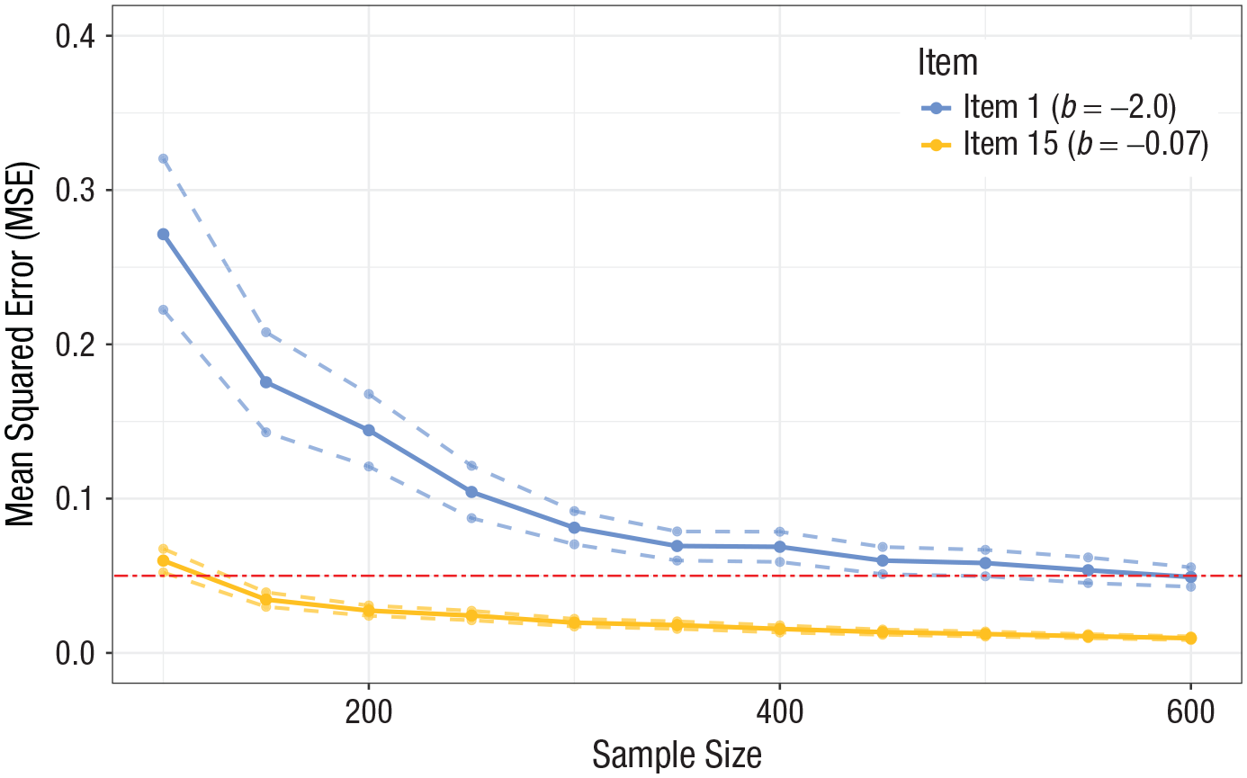
Mean square error of item difficulties with 95% confidence intervals depending on the sample size. Dashed lines indicate the margin of error (MSE ± 1.96 × Monte Carlo standard error).

Example 2: personality-test validation with randomized item sampling

Determining the data generation for the complete data set

In the second example, we describe the validation of a newly developed computerized personality test with a forced-choice response format comparable with the Eysenck Personality Inventory (e.g., “Do you prefer reading to going out?”; yes/no). Forced-choice personality items offer several advantages over rating scales, including minimizing the likelihood of response-pattern bias (Brown & Maydeu-Olivares, 2011), increasing test reliability and validity (Stark et al., 2005), and encouraging honest responses from participants (Christiansen et al., 2005). In this example, forced-choice items measuring extraversion that are randomly selected from a larger 30-item pool are considered. The latent trait was assumed to correlate with an external metric variable at ρ = .50, and accordingly, the persons’ abilities are generated using a multivariate normal distribution. The difficulty parameters are defined as in the first example, and the discrimination parameters are drawn from a log-normal distribution to reflect realistic variation with positive skewness typically observed in empirical data.

Defining the test design and the process of missing values

The items of the computer-administered personality test are randomly drawn from a larger item pool, generally ensuring complete coverage of item covariances for a nontrivial sample size. Such a random sampling design is, for example, used in the Synthetic Aperture Personality Assessment project (Condon et al., 2017) to maximize the breadth and depth of personality assessment by administering a wide range of items. In this simulation, three levels of missingness are examined: 0% (equivalent to 30 administered items), 33% (equivalent to 20 administered items), and 67% (equivalent to 10 administered items). In the simulation, the complete data are generated first, and then observations are deleted under the assumption of missing completely at random (MCAR⁵).

Selecting the IRT model and the parameter of interest

The model to be estimated is a unidimensional 2PL model with a regression of the latent trait on the z-standardized criterion. The parameter of interest is the standard error of the regression coefficient, which corresponds to the correlation between extraversion and the metric criterion. In addition to the sample size, the amount of missing data is also varied to determine the optimal test design for estimating the standard error with sufficient precision. This example illustrates that the sample-size estimation is also affected by other factors, such as the test design.

Setting up the Monte Carlo simulation

The standard deviation of the standard error of the correlation derived from 500 iterations was low (σ = .0052), also in the most demanding condition (n = 200, missing rate = 67%). Combined with a specified level of accuracy (δ = .001) and a significance level (α = .05), this implies a number of required iterations of approximately 104. The simulation is run for different sample sizes between 200 and 700 (in increments of 50) with three levels of missing rates (0%, 33%, 67%).

Results and interpretation

Figure 2 shows the average standard error of the correlation across all iterations between the forced-choice personality test and the metric criterion. For the full 30-item questionnaire, the threshold is reached with about 500 participants. The lines for none and one-third of missing items are close together, indicating that the absolute number of items is decisive and that a precise estimate of the standard error is already obtained with 20 items. Note, however, that the effect of missingness is not linear. The decision as to whether it is beneficial to include more items per participant or to recruit more participants who work on smaller item sets depends on the specific circumstances of the study and can be determined through a cost analysis (Zimmer & Debelak, 2023; Zimmer et al., 2024).

Fig. 2.

Average standard error of the correlation depending on the sample size and number of items. The plot shows the average standard error of the correlation as a function of the sample size and the number of items, with varying percentages of missingness. The red dashed line indicates the target standard error of 0.05.

Example 3: conditional reliabilities of three clinical measures

Determining the data generation for the complete data set

In the third example, we describe how to determine the sample size required to estimate the conditional reliability of a test with a specified precision using the GRM (Samejima, 1969). The simulated data are based on the empirical item parameters of three popular clinical-depression measures, as reported in the study by Choi et al. (2014). The measures differ in the number of items; the Beck Depression Inventory–II (BDI) has 21 items, the Center for Epidemiological Studies Depression Scale (CESD) has 20 items, and the Patient Health Questionnaire (PHQ) has nine items. All items are answered on a 4-point, ordered response scale; for example, CESD-1, “I was bothered by things that usually don’t bother me,” had responses from 0 (rarely or none of the time) to 3 (most or all of the time). These instruments are designed to measure accurately in an elevated range of the trait distribution because they are used to screen patients for clinically relevant levels of depression. In clinical assessment, symptom severity is typically characterized as mild (0.5 < θ < 1.0), moderate (1.0 < θ < 2.0), and severe (θ > 2.0).

In contrast to classical test theory, which assumes that a single reliability estimate applies universally to all levels of a trait, IRT estimates reliability conditionally, specific to a given trait level (e.g., different levels of depressivity; see Fig. 3). The true conditional reliability estimate (ρ_true) can be calculated from the item parameters: High discrimination parameters (a_i) enhance reliability by better differentiating between individuals at specific trait levels, and difficulty parameters (b_i) determine the trait levels at which items are most informative. The accuracy of the estimated conditional reliability (ρ_est) depends largely on the sample size.

Fig. 3.

True conditional reliability across three measures of depressivity. The true conditional reliability calculated from the item parameters is shown. The gray vertical line indicates the value of the latent trait (θ = 2.0) at which the standard error of the conditional reliability is examined.

Defining the test design and the process of missing values

It is assumed that respondents are randomly administered two of the three depression instruments. Thus, this is a special form of a reciprocal linking design in which the linking items comprise the complete instruments.

Selecting the IRT model and the parameter of interest

The GRM is used to analyze ordered categorical responses, typically encountered in clinical-rating scales. The model estimates the probability that respondents will select a particular response category based on their underlying trait level; each item has multiple thresholds corresponding to the different response categories (see Equation 2). The true conditional reliability (ρ_true) at a given point in the trait distribution (θ = 2.0), calculated from the item parameters, was .97 for the BDI, .96 for the CESD, and .91 for the PHQ. To quantify the accuracy of the estimated reliability, the root mean square error (RMSE) of the reliability is used, $R M S E (ρ) = \sqrt{M ({(ρ_{e s t} - ρ_{t r u e})}^{2})}$ .

Setting up the Monte Carlo simulation

Using an estimated standard deviation for the RMSE of the estimated reliability (σ = .012) derived from 500 iterations, a specified level of accuracy (δ = .001), and a significance level (α = .05), we found that the number of iterations required is approximately 553. The simulation is run for different total sample sizes between 300 and 1,050 (in increments of 75). Because of the chosen test design, the sample size for each individual measure is two-thirds of the total sample size (i.e., 200–700 in increments of 50).

Results and interpretation

For the longer measures, CESD and BDI, the conditional reliability at the relevant trait level is higher, and the associated RMSE is lower than for the short measure. For the PHQ, the required accuracy of RMSE ≤ .01 is achieved with a sample size of approximately 600 participants who completed the instrument (or a total sample size of 900 participants; see Fig. 4). If the accuracy of the conditional reliability of all instruments is to be identical, groups of unequal size would have to complete the instruments.

Fig. 4.

Accuracy of the conditional reliability estimate at the boundary between moderate and severe symptom severity depending on sample size. The lines for the BDI and CESD largely overlap. BDI = Beck Depression Inventory–II; CESD = Center for Epidemiological Studies Depression Scale; PHQ = Patient Health Questionnaire.

Summary and Outlook

IRT offers a versatile yet often underused toolbox for constructing, evaluating, and refining psychological measures. Current applications range from educational assessment (Hori et al., 2022) to clinical symptom evaluation (Balsis et al., 2017; Thomas, 2019) and organizational-behavior research (Lang & Tay, 2021). Despite its versatility, the IRT framework has not yet been fully embraced across all areas of psychology. A major reason for this may be uncertainty about the sample size required to estimate complex IRT models with many parameters or missing data, especially compared with more familiar factor-analytic approaches (ten Holt et al., 2010). This hesitation is unfortunate given the potential of IRT in many contexts: For example, IRT is prominently used in the Patient-Reported Outcomes Measurement Information System (Cella et al., 2010) to capture patients’ perspectives on their health, quality of life, and treatment outcomes through computer-adaptive testing, thereby, reducing testing time, response burden, and potential memory bias.

Since its invention, the IRT framework has continuously been expanded, now encompassing a wide range of models for specific purposes. For example, cognitive-diagnosis models (Templin & Henson, 2006) assess whether students have mastered specific cognitive skills, conjoint IRT (Klein Entink et al., 2009) integrates response times alongside the accuracy of an answer, and multidimensional zero-inflated GRMs (Magnus & Garnier-Villarreal, 2022) examine symptom frequencies of psychopathology in community samples in which endorsements are rare. To address concerns regarding the use of IRT, we advocate for a simulation-based approach to sample-size planning, tailored to the unique conditions of a given study (for similar calls, see Zimmer & Debelak, 2023; Zimmer et al., 2024).

In this tutorial, we have presented a guide with 10 key decisions, organized into four steps. In the first step, the data-generation process for the complete data set needs to be determined. This requires thinking about the item types included in the test, the assumed response process, and the item parameters (e.g., difficulty, discrimination) to be estimated. The second step involves specifying the concrete test design (e.g., booklet design) and how items are administered (e.g., linking design) to clarify potential processes leading to different types of missing values (MCAR, MAR). In the third step, the IRT model (e.g., 2PL, GRM) and the parameters of interest (e.g., item difficulty) are chosen depending on the research question and the conditions specified in the previous steps. In the fourth step, the design of the Monte Carlo simulation needs to be specified, which includes determining the number of required iterations to obtain stable estimates of the parameters of interest and deciding on the range of sample sizes to consider. To assist researchers in setting up their own simulation, the four steps described in our guide were illustrated with several examples, covering a wide range of applications, that stretched from the simple Rasch modeling of a one-dimensional performance test administered in a linked test design (Example 1) to the criterion validation in a multidimensional 2PL model with randomized item selection (Example 2) to the conditional reliability in a GRM (Example 3). Additional application examples with accompanying syntax are available in the supplement material (https://ulrich-schroeders.github.io/IRT-sample-size/).

Although we agree that simulation-based sample-size planning is more complex and time-consuming than relying on simple rules of thumb provided in the psychometric literature (e.g., DeMars, 2010; Valdivia & Dai, 2024), properly specified simulations will lead to more accurate sample-size estimates for a planned study and ultimately to more robust results because specifics of the research question, test design, and data conditions together influence the required sample size in unique ways. To further lower the technical hurdle for performing IRT sample estimation, a next step could be to make the functions outlined in this tutorial more flexible (e.g., with respect to specifying different test designs) and to develop user-friendly software (e.g., a shiny app). In addition, the functionality of the syntax could be extended to use cases such as adaptive testing with missing data processes that depend on the ability of the person (e.g., using the R packages catR and mirtCAT; see Magis et al., 2017) or modern procedures for differential-item-functioning analyses to address issues of measurement invariance across categorical and metric variables (e.g., based on the R packages GPCMlasso, Schauberger & Mair, 2020; or psychotree, Strobl et al., 2015).

The checklist provided in Table 2 summarizes critical decisions that researchers must make when planning a simulation study to determine the required sample size, which will hopefully assist in the preparation of preregistrations and registered reports and during the review process. However, this checklist should be seen as a flexible template rather than a rigid prescription. Researchers are advised to adapt the framework to fit their specific study conditions. For example, depending on the research question, different IRT models, including multidimensional and mixed models, might need to be specified, or the focus of the simulation may need to shift to a different parameter, such as the mean difference between a treatment group and a control group. In addition, it might be interesting to examine sample-size requirements from a cost-benefit perspective (Zimmer & Debelak, 2023; Zimmer et al., 2024) to decide whether improving precision by assessing more respondents outweighs the additional costs (e.g., in terms of time, money, and participant burden).

Researchers should be reminded that the accuracy of simulations depends on how well the model assumptions reflect real-world conditions and adequately account for the complexities of empirical data. For example, in practice, a measurement instrument may deviate from the assumed unidimensional model (e.g., negatively worded items may introduce method-specific variance; see Gnambs & Schroeders, 2020), or participants may vary in their engagement in answering the questions (e.g., careless/insufficient effort responding; see Schroeders et al., 2022). Simulations often assume more ideal data conditions than empirical data sets, which are plagued by such item- or person-specific effects. Therefore, sample-size planning should take these conditions into account by varying different model assumptions in the Monte Carlo simulation to examine the extent to which they affect the required sample-size estimation. We hope the framework presented in this tutorial will help researchers to do so and encourage the wider adoption of IRT in psychological research, leading to improved measurement practices.

Footnotes

Acknowledgements

We confirm that the work conforms to Standard 8 of the American Psychological Association’s Ethical Principles of Psychologists and Code of Conduct.

Transparency

Action Editor: Yasemin Kisbu-Sakarya

Editor: David A. Sbarra

Author Contributions

Ulrich Schroeders: Conceptualization; Formal analysis; Methodology; Software; Writing – original draft; Writing – review & editing.

Timo Gnambs: Conceptualization; Formal analysis; Methodology; Software; Writing – review & editing.

ORCID iDs

Ulrich Schroeders

Timo Gnambs

Notes

References

Balsis

Ruchensky

J. R.

Busch

A. J.

(2017). Item response theory applications in personality disorder research. Personality Disorders: Theory, Research, and Treatment, 8(4), 298–308. https://doi.org/10.1037/per0000209

Belzak

W. C.

(2020). Testing differential item functioning in small samples. Multivariate Behavioral Research, 55(5), 722–747. https://doi.org/10.1080/00273171.2019.1671162

Berrío

Á. I.

Gomez-Benito

Arias-Patiño

E. M

. (2020). Developments and trends in research on methods of detecting differential item functioning. Educational Research Review, 31, Article 100340. https://doi.org/10.1016/j.edurev.2020.100340

Birnbaum

(1968). Some latent trait models and their use in inferring an examinee’s ability. In Lord

F. M.

Novick

M. R.

(Eds.), Statistical theories of mental test scores (pp. 397–479). Addison-Wesley.

Bock

R. D.

(1972). Estimating item parameters and latent ability when responses are scored in two or more nominal categories. Psychometrika, 37, 29–51. https://doi.org/10.1007/BF02291411

Brown

Maydeu-Olivares

(2011). Item response modeling of forced-choice questionnaires. Educational and Psychological Measurement, 71(3), 460–502. https://doi.org/10.1177/0013164410375112

Brown

Maydeu-Olivares

(2013). How IRT can solve problems of ipsative data in forced-choice questionnaires. Psychological Methods, 18(1), 36–52. https://doi.org/10.1037/a0030641

Burton

Altman

D. G.

Royston

Holder

R. L.

(2006). The design of simulation studies in medical statistics. Statistics in Medicine, 25(24), 4279–4292. https://doi.org/10.1002/sim.2673

Cella

Yount

Rothrock

Gershon

Cook

Reeve

Ader

Fries

J. F.

Bruce

Rose

(2010). The Patient-Reported Outcomes Measurement Information System (PROMIS): Progress of an NIH roadmap cooperative group during its first two years. Medical Care, 45(5, Suppl. 1), S3–S11. https://doi.org/10.1097/MLR.0b013e3181c59548

10.

Chalmers

R. P.

(2012). mirt: A multidimensional item response theory package for the R environment. Journal of Statistical Software, 48(6), 1–29. https://doi.org/10.18637/jss.v048.i06

11.

Choi

S. W.

Schalet

Cook

K. F.

Cella

(2014). Establishing a common metric for depressive symptoms: Linking the BDI-II, CES-D, and PHQ-9 to PROMIS Depression. Psychological Assessment, 26(2), 513–527. https://doi.org/10.1037/a0035768

12.

Christiansen

N. D.

Burns

G. N.

Montgomery

G. E.

(2005). Reconsidering forced-choice item formats for applicant personality assessment. Human Performance, 18(3), 267–307. https://doi.org/10.1207/s15327043hup1803_4

13.

Clifton

J. D. W.

(2020). Managing validity versus reliability trade-offs in scale-building decisions. Psychological Methods, 25(3), 259–270. https://doi.org/10.1037/met0000236

14.

Condon

D. M.

Roney

Revelle

(2017). A SAPA project update: On the structure of phrased self-report personality items. Journal of Open Psychology Data, 5, Article 3. https://doi.org/10.5334/jopd.32

15.

Cuhadar

(2022). Sample size requirements for parameter recovery in the 4-Parameter logistic model. Measurement: Interdisciplinary Research and Perspectives, 20(2), 57–72. https://doi.org/10.1080/15366367.2021.1934805

16.

De Ayala

R. J

. (2022). The theory and practice of item response theory. The Guilford Press.

17.

De Ayala

R. J.

Sava-Bolesta

. (1999). Item parameter recovery for the nominal response model. Applied Psychological Measurement, 23(1), 3–19. https://doi.org/10.1177/01466219922031130

18.

DeMars

C. E.

(2003). Sample size and the recovery of nominal response model item parameters. Applied Psychological Measurement, 27(4), 275–288. https://doi.org/10.1177/0146621603027004003

19.

DeMars

C. E.

(2010). Item response theory. Oxford University Press.

20.

Enders

C. K.

(2023). Missing data: An update on the state of the art. Psychological Methods. Advance online publication. https://doi.org/10.1037/met0000563

21.

Finch

French

B. F.

(2019). A comparison of estimation techniques for IRT models with small samples. Applied Measurement in Education, 32(2), 77–96. https://doi.org/10.1080/08957347.2019.1577243

22.

Flake

J. K.

Fried

E. I.

(2020). Measurement schmeasurement: Questionable measurement practices and how to avoid them. Advances in Methods and Practices in Psychological Science, 3(4), 456–465. https://doi.org/10.1177/2515245920952393

23.

Forthmann

Gühne

Doebler

(2020). Revisiting dispersion in count data item response theory models: The Conway–Maxwell–Poisson counts model. British Journal of Mathematical and Statistical Psychology, 73, 32–50. https://doi.org/10.1111/bmsp.12184

24.

Frey

Hartig

Rupp

A. A.

(2009). An NCME instructional module on booklet designs in large-scale assessments of student achievement: Theory and practice. Educational Measurement: Issues and Practice, 28(3), 39–53. https://doi.org/10.1111/j.1745-3992.2009.00154.x

25.

Gnambs

Schroeders

(2020). Cognitive abilities explain wording effects in the Rosenberg Self-Esteem Scale. Assessment, 27(2), 404–418. https://doi.org/10.1177/1073191117746503

26.

Gonzalez

Rutkowski

(2010). Principles of multiple matrix booklet designs and parameter recovery in large-scale assessments. In Hastedt

von Davier

(Eds.), IERI monograph series: Issues and methodologies in large-scale assessments (Vol. 3, pp. 125–156). IEA-ETS Research Institute.

27.

Holman

Glas

C. A. W.

De Haan

R. J.

(2003). Power analysis in randomized clinical trials based on item response theory. Controlled Clinical Trials, 24(4), 390–410. https://doi.org/10.1016/S0197-2456(03)00061-8

28.

Hori

Fukuhara

Yamada

(2022). Item response theory and its applications in educational measurement Part II: Theory and practices of test equating in item response theory. WIREs Computational Statistics, 14(3), Article e1543. https://doi.org/10.1002/wics.1543

29.

Joshi

Pustejovsky

J. M.

(2024). simhelpers: Helper functions for simulation studies (Version 0.3.0) [Computer software]. https://doi.org/10.32614/CRAN.package.simhelpers

30.

Klein Entink

R. H.

Fox

J.-P.

van Der Linden

W. J

. (2009). A multivariate multilevel approach to the modeling of accuracy and speed of test takers. Psychometrika, 74(1), 21–48. https://doi.org/10.1007/s11336-008-9075-y

31.

Kolen

M. J.

Brennan

R. L.

(2014). Test equating, scaling, and linking: Methods and practices. Springer.

32.

König

Spoden

Frey

(2020). An optimized Bayesian hierarchical two-parameter logistic model for small-sample item calibration. Applied Psychological Measurement, 44(4), 311–326. https://doi.org/10.1177/0146621619893786

33.

Kutscher

Eid

Crayen

(2019). Sample size requirements for applying mixed polytomous item response models: Results of a Monte Carlo simulation study. Frontiers in Psychology, 10, Article 2494. https://doi.org/10.3389/fpsyg.2019.02494

34.

Lang

J. W.

Tay

(2021). The science and practice of item response theory in organizations. Annual Review of Organizational Psychology and Organizational Behavior, 8(1), 311–338. https://doi.org/10.1146/annurev-orgpsych-012420-061705

35.

Magis

Yan

Von Davier

A. A.

(2017). Computerized adaptive and multistage testing with R: Using packages catR and mstR. Springer. https://doi.org/10.1007/978-3-319-69218-0

36.

Magnus

B. E.

Garnier-Villarreal

(2022). A multidimensional zero-inflated graded response model for ordinal symptom data. Psychological Methods, 27(2), 261–279. https://doi.org/10.1037/met0000395

37.

Markus

K. A.

Borsboom

(2013). Reflective measurement models, behavior domains, and common causes. New Ideas in Psychology, 31(1), 54–64. https://doi.org/10.1016/j.newideapsych.2011.02.008

38.

Morris

T. P.

White

I. R.

Crowther

M. J.

(2019). Using simulation studies to evaluate statistical methods. Statistics in Medicine, 38(11), 2074–2102. https://doi.org/10.1002/sim.8086

39.

Moshagen

Bader

(2024). semPower: General power analysis for structural equation models. Behavior Research Methods, 56, 2901–2922. https://doi.org/10.3758/s13428-023-02254-7

40.

Muthén

L. K.

Muthén

B. O.

(2002). How to use a Monte Carlo study to decide on sample size and determine power. Structural Equation Modeling, 9(4), 599–620. https://doi.org/10.1207/S15328007SEM0904_8

41.

R Core Team. (2024). R: A language and environment for statistical computing [Computer software]. https://www.R-project.org/

42.

Rasch

(1960). Probabilistic models for some intelligence and attainment tests. The Danish Institute of Education Research.

43.

Reise

S. P.

Waller

N. G.

(2003). How many IRT parameters does it take to model psychopathology items? Psychological Methods, 8, 164–184. https://doi.org/10.1037/1082-989x.8.2.164

44.

Robitzsch

Kiefer

(2024). TAM: Test analysis modules. R package (Version 4.2–21) [Computer software]. https://doi.org/10.32614/CRAN.package.TAM

45.

Robitzsch

Lüdtke

(2022). Some thoughts on analytical choices in the scaling model for test scores in international large-scale assessment studies. Measurement Instruments for the Social Sciences, 4(1), Article 9. https://doi.org/10.1186/s42409-022-00039-w

46.

Samejima

(1969). Estimation of latent ability using a response pattern of graded scores. Psychometrika, 34(Suppl. 1), 1–97. https://doi.org/10.1007/BF03372160

47.

Schafer

J. L.

Graham

J. W.

(2002). Missing data: Our view of the state of the art. Psychological Methods, 7(2), 147–177. https://doi.org/10.1037//1082-989X.7.2.147

48.

Scharl

Gnambs

(2024). The impact of different methods to correct for response styles on the external validity of self-reports. European Journal of Psychological Assessment, 40(1), 13–21. https://doi.org/10.1027/1015-5759/a000731

49.

Schauberger

Mair

(2020). A regularization approach for the detection of differential item functioning in generalized partial credit models. Behavior Research Methods, 52, 279–294. https://doi.org/10.3758/s13428-019-01224-2

50.

Schroeders

Loos

Wiedemann

Jankowsky

(2024). Is it just a game? Development and validation of a deductive version of mastermind as measure of reasoning ability. European Journal of Psychological Assessment. Advance online publication. https://doi.org/10.1027/1015-5759/a000855

51.

Schroeders

Schmidt

Gnambs

(2022). Detecting careless responding in survey data using stochastic gradient boosting. Educational and Psychological Measurement, 82(1), 29–56. https://doi.org/10.1177/00131644211004708

52.

Sen

Cohen

A. S.

(2023). The impact of sample size and various other factors on estimation of dichotomous mixture IRT models. Educational and Psychological Measurement, 83(3), 520–555. https://doi.org/10.1177/00131644221094325

53.

Sheng

(2013). An empirical investigation of Bayesian hierarchical modeling with unidimensional IRT models. Behaviormetrika, 40(1), 19–40. https://doi.org/10.2333/bhmk.40.19

54.

Stark

Chernyshenko

O. S.

Drasgow

(2005). Examining the effects of differential item functioning on personality assessments. Journal of Applied Psychology, 90(4), 715–726. https://doi.org/10.1037/0021-9010.90.4.715

55.

Steger

Jankowsky

Schroeders

Wilhelm

(2023). The road to hell is paved with good intentions: How common practices in scale construction hurt validity. Assessment, 30(6), 1811–1824. https://doi.org/10.1177/10731911221124846

56.

Strobl

Kopf

Zeileis

(2015). Rasch trees: A new method for detecting differential item functioning in the Rasch model. Psychometrika, 80(2), 289–316. https://doi.org/10.1007/s11336-013-9388-3

57.

Tay

Drasgow

Rounds

Williams

B. A.

(2009). Fitting measurement models to vocational interest data: Are dominance models ideal? Journal of Applied Psychology, 94(5), 1287–1304. https://doi.org/10.1037/a0015899

58.

Templin

J. L.

Henson

R. A.

(2006). Measurement of psychological disorders using cognitive diagnosis models. Psychological Methods, 11(3), 287–305. https://doi.org/10.1037/1082-989X.11.3.287

59.

ten Holt

J. C.

van Duijn

M. A.

Boomsma

. (2010). Scale construction and evaluation in practice: A review of factor analysis versus item response theory applications. Psychological Test and Assessment Modeling, 52(3), 272–297.

60.

Thissen

Steinberg

(1986). A taxonomy of item response models. Psychometrika, 51, 567–577. https://doi.org/10.1007/BF02295596

61.

Thomas

M. L.

(2019). Advances in applications of item response theory to clinical assessment. Psychological Assessment, 31(12), 1442–1455. https://doi.org/10.1037/pas0000597

62.

Valdivia

S. D.

Dai

(2024). Number of response categories and sample size requirements in polytomous IRT models. The Journal of Experimental Education, 92(1), 154–185. https://doi.org/10.1080/00220973.2022.2153783

63.

van der Linden

W. J

. (Ed.). (2018). Handbook of item response theory. CRC Press.

64.

Wahl

Löwe

Bjorner

J. B.

Fischer

Langs

Voderholzer

Aita

S. A.

Bergemann

Brähler

Rose

(2014). Standardization of depression measurement: A common metric was developed for 11 self-report depression measures. Journal of Clinical Epidemiology, 67(1), 73–86. https://doi.org/10.1016/j.jclinepi.2013.04.019

65.

Wang

Y. A.

Rhemtulla

(2021). Power analysis for parameter estimation in structural equation modeling: A discussion and tutorial. Advances in Methods and Practices in Psychological Science, 4(1), 599–620. https://doi.org/10.1177/25152459209182

66.

Welling

Gnambs

Carstensen

C. H.

(2024). Identifying disengaged responding in multiple-choice items: Extending a latent class item response model with novel process data indicators. Educational and Psychological Measurement, 84(2), 314–339. https://doi.org/10.1177/00131644231169211

67.

Wolf

E. J.

Harrington

K. M.

Clark

S. L.

Miller

M. W.

(2013). Sample size requirements for structural equation models: An evaluation of power, bias, and solution propriety. Educational and Psychological Measurement, 73(6), 913–934. https://doi.org/10.1177/0013164413495237

68.

Zimmer

Debelak

(2023). Simulation-based design optimization for statistical power: Utilizing machine learning. Psychological Methods. Advance online publication. https://doi.org/10.1037/met0000611

69.

Zimmer

Henninger

Debelak

(2024). Sample size planning for complex study designs: A tutorial for the mlpwr package. Behavior Research Methods, 56, 5246–5263. https://doi.org/10.3758/s13428-023-02269-0

70.

Zimny

Schroeders

Wilhelm

(2024). Ant colony optimization for parallel test assembly. Behavior Research Methods, 56, 5834–5848. https://doi.org/10.3758/s13428-023-02319-7

Sample-Size Planning in Item-Response Theory: A Tutorial

Abstract

Keywords

A Short Recap on IRT Modeling

Simulation-Based Sample-Size Determination for IRT Analyses

The Present Tutorial

Example 1: piloting an ability test with a linked test design

Determining the data generation for the complete data set

Defining the test design and the process of missing values

Selecting the IRT model and the parameter of interest

Setting up the Monte Carlo simulation

Results and interpretation

Example 2: personality-test validation with randomized item sampling

Determining the data generation for the complete data set

Defining the test design and the process of missing values

Selecting the IRT model and the parameter of interest

Setting up the Monte Carlo simulation

Results and interpretation

Example 3: conditional reliabilities of three clinical measures

Determining the data generation for the complete data set

Defining the test design and the process of missing values

Selecting the IRT model and the parameter of interest

Setting up the Monte Carlo simulation

Results and interpretation

Summary and Outlook

Footnotes

Acknowledgements

Transparency

ORCID iDs

Notes

References