A Methodological Framework for Stimuli Control: Insights From Numerical Cognition

Abstract

The stimuli presented in cognitive experiments have a crucial role in the ability to isolate the underlying mechanism from other interweaved mechanisms. New ideas aimed at unveiling cognitive mechanisms are often realized through introducing new stimuli. This, in turn, raises challenges in reconciling results to literature. We demonstrate this challenge in the field of numerical cognition. Stimuli used in this field are designed to present quantity in a non symbolic manner. Physical properties, such as surface area and density, inherently correlate with quantity, masking the mechanism underlying numerical perception. Different generation methods (GMs) are used to control these physical properties. However, the way a GM controls physical properties affects numerical judgments in different ways, compromising comparability and the pursuit of cumulative science. Here, using a novel data-driven approach, we provide a methodological review of non symbolic stimuli GMs developed since 2000. Our results reveal that the field thrives and that a wide variety of GMs are tackling new methodological and theoretical ideas. However, the field lacks a common language and means to integrate new ideas into the literature. These shortcomings impair the interpretability, comparison, replication, and reanalysis of previous studies that have considered new ideas. We present guidelines for GMs relevant also to other fields and tasks involving perceptual decisions, including (a) defining controls explicitly and consistently, (b) justifying controls and discussing their implications, (c) considering stimuli statistical features, and (d) providing complete stimuli set, matching responses, and generation code. We hope these guidelines will promote the integration of findings and increase findings’ explanatory power.

Cognitive research aims to understand distinct cognitive capacities. Controlling experimental stimuli ensures their relevance to the studied capacity, regardless of the modality used, and their ecological validity (Bays et al., 2009; Blandford et al., 2008; Boring, 1954; Eriksen, 1980; Pelham & Blanton, 2007; Rangelov et al., 2022; Torday & Baluška, 2019; Waskom et al., 2019). Stimuli control is a cornerstone of experimental control, helping cognitive scientists to ensure that their results are not artifactual. Building on the foundational concept of stimuli control, we elucidate its critical role in studying visual numerical perception (numerosity). This data-driven methodological review focuses on methods to generate controlled non symbolic numerical stimuli for numerical comparisons. Yet this review’s conclusions apply to many other fields and tasks involving perceptual decisions.

Stimuli Control in Non Symbolic Numerical-Comparison Studies

Recent numerical-comparison studies have struggled to control the physical properties of non symbolic arrays and the physical properties’ correlations with the array’s quantity. An array of items can be described by its number of items or by its physical properties. The physical properties of any item array have a natural and inherent correlation with the array’s quantity (Dehaene, 1997; Leibovich et al., 2017; Mehler & Bever, 1967). Increasing or decreasing the number of items necessarily changes at least one of the array’s physical properties (see Fig. 1 and De Marco & Cutini, 2020; DeWind et al., 2015; Leibovich & Henik, 2013; Zanon et al., 2021). Consider three large apples lying on the kitchen counter. Adding a fourth large apple would increase the total surface area and circumference of the apples’ stack (array). If the fourth apple is larger than the original three apples, the average array’s surface area circumference, diameter, and so on would also increase. The addition of the fourth apple would also reduce the average distance (i.e., interdistance) between the apples. Changing the number of apples in the stack would also change density, the perimeter of the polygon surrounding all the array’s items, and so on. The physical properties discussed are only part of the properties that could be considered (see full list in Fig. 5). Importantly, property changes cannot be linearly predicted from changes in numerosity alone.

Fig. 1.

The natural association between physical properties and quantity is not a simple linear correlation.

Early studies have shown an association between performance in numerical judgments and the physical properties of the presented stimuli (French, 1953; Frith & Frith, 1972; Piaget, 1968). In the contemporary study of numerical cognition, the physical properties of a numerical array are considered in two opposing manners. Some treat them as a biasing factor, distracting researchers from the thing they want to study—the ability to judge numerosity (e.g., Halberda et al., 2008 ¹ ; Halberda & Feigenson, 2008; Piazza et al., 2004 ² ). Others treat them as a key to understanding numerical capacity (Gebuis & Reynvoet, 2011a, 2011b; Leibovich et al., 2017). Regardless of their view of numerical cognition, researchers must address the natural correlation between the array’s physical properties and its quantity to prevent confounds. Importantly, there are abundant ways to create non symbolic numerical stimuli relying on different theoretical and methodological prisms (DeWind et al., 2015; Gebuis & Reynvoet, 2011a, 2011b; Piazza et al., 2004; Salti et al., 2017). The different ways stimuli are created change the correlations between numerical and physical properties. The different correlations between numerical and physical properties bias behavioral and neuronal results (Clayton et al., 2015; DeWind & Brannon, 2016; Gebuis & Reynvoet, 2011a, 2011b; Kuzmina & Malykh, 2022; Leibovich et al., 2017; Salti et al., 2017; Smets et al., 2015). The different correlations between numerical and physical properties make it harder to compare different studies (Clayton et al., 2015; Smets et al., 2015) and limit the ability to examine previous studies through new theoretical prisms.

Non symbolic numerical stimuli are multifaceted and can be categorized according to different taxonomies, for example, according to a global-local categorization (e.g., Guy & Medioni, 1993; Navon, 1977) or intrinsic–extrinsic categorization (DeWind et al., 2015; Gebuis & Reynvoet, 2011a, 2011b; Salti et al., 2017). Individual physical properties can also be defined in multiple ways. For example, there are six different definitions for “density” in the literature (see Qualitative Analysis section). The diverse ways to address, control, manipulate, and analyze physical properties make it harder to achieve a common scientific ground (Stalnaker, 2002). The lack of common ground hinders efficient comparisons of results coming from different studies that used different methods to generate stimuli. Hereafter, we denote the generation methods to generate non symbolic numerical stimuli as GMs. A GM is defined as a unique algorithm for creating visual non symbolic stimuli according to predefined numerical and physical parameters. Different GMs use different experimental controls and manipulations that produce different correlations between numerical and physical properties (Gebuis & Reynvoet, 2011a; Katzin et al., 2019; Salti et al., 2017). The different correlations might bias the results of studies. Smets et al. (2015) found that two different GMs suggested by Piazza and Dehaene and by Gebuis and Reynvoet led to different Weber fractions and performance accuracy (Gebuis & Reynvoet, 2011a; Piazza et al., 2004). Simply put, the Weber fraction measures the numerical comparison acuity (Chen & Li, 2014; Leibovich et al., 2017; Smets et al., 2015). It is quantified by dividing the smallest (reliably) discriminable difference in quantity between the compared arrays by the quantity of the smaller array, used as a reference. The different correlations also lead to different congruity effects. A congruity effect is quantified by the performance difference (usually in reaction time or accuracy) between incongruent and congruent trials. In the canonical congruity effect, responses are faster and more accurate for congruent trials in which the more numerous array is also larger in its physical properties (e.g., total surface area) and responses are slower for incongruent trials in which the less numerous array is larger in its physical properties (Leibovich et al., 2017; Rousselle et al., 2004). Clayton et al. (2015) also found that two different GMs led to different accuracy and congruity effects. When the stimuli were created using Gebuis and Reynvoet’s (2011a) GM, participants exhibited the canonical congruity effect, whereas the Panamath GM (Halberda et al., 2008; Halberda & Feigenson, 2008) led to the opposite congruency effect. Using stimuli sets created by the Panamath GM, the participants’ accuracy was higher in incongruent trials than in congruent trials. When Clayton et al. (2015) compared the stimuli produced by Gebuis and Reynvoet’s GM to the Panamath GM stimuli (Halberda et al., 2008; Halberda & Feigenson, 2008), they discovered that the relationship between the arrays’ convex hull area, total surface area, and quantity were different between the two different stimuli sets. To conclude, comparing the results coming from different experiments with stimuli generated by different GMs is limited.

The variety of GMs also limits the ability to examine previous studies through new theoretical prisms. For example, Yousif and Keil (2019) suggested that arrays’ additive area, defined as the sum of the items’ height and width, has a role in numerical judgments (see Fig. 5 and Park’s, 2022, critique on the additive area, discussion section). Previous studies have not recorded data on arrays’ additive area, nor have they provided their stimuli. Therefore, it is impossible to test this idea retrospectively because there is no way to extract the relevant information from previous studies. Another example is Maldonado Moscoso et al. (2023), who proposed that symmetrical arrays are processed differently than random arrays. A symmetric array has two identical halves. Previous studies have not recorded data on arrays’ symmetry or provided sufficient details on the items’ spatial arrangement and size, nor have they provided their stimuli. Therefore, it is impossible to test how symmetry affects numerical decisions retrospectively. Another example comes from our own experience. We lately suggested that the shape of the convex hull is important for numerical judgments (Katzin et al., 2019; Shilat et al., 2021). Previous studies have not recorded data on the shape of the convex hull and have not provided their stimuli. Therefore, it is impossible to test this idea retrospectively. Science evolves, and new ideas constantly emerge. To prioritize new ideas, it is best to test them using diverse methods. Testing new ideas on previously published data could help the future scientist and enable more rapid progression.

The Current Review

The purpose of the current review is to create common ground for future studies and to provide tools to test new ideas on already existing data. We start by describing the current state of the field in terms of a common language and then map the different controls employed by the various GMs. For each GM, we examined how the physical properties were defined and how they were controlled. This was followed by a quantitative analysis of the distribution of the frequency of these different controls. Describing the field and mapping it provided a data-driven review of the different GMs.

Method

Procedure overview

We studied GMs of non symbolic numerical stimuli designed to control the physical properties of non symbolic numerical stimuli. We started by identifying and collecting the different GMs. This provided qualitative raw data on the different ways to control physical properties. Human annotators tagged the different controls in each of the identified methods, making the qualitative data suitable for quantitative analysis of the distributions and trends in the GMs’ control over physical properties. Figure 2 presents an overview of the structure and pipeline of this review. We focused on GMs published between the years 2000 and 2021. Focusing on these years allowed a broad and exhaustive look, on one hand, and on the other, narrowed it to relevant GMs used in contemporary research.

Fig. 2.

The structure and pipeline of this review. The workflow of constructing the current review started by creating a database of 32 non symbolic numerical stimuli GMs published since 2000 (see section GMs Database). Analyzing the controls imposed by these GMs allowed us to identify five overarching control types applied to 16 properties (see section Identifying the Controls). Then, we tagged the individual GMs’ controls. We performed a qualitative analysis of the GMs’ provided data types, control definitions, terminology, and reliance on theoretical justification (see section Qualitative Analysis). Building on the tagged data and qualitative analysis, we quantitatively analyzed the GMs’ control. Finally, deriving from our analysis, we provided guidelines for GMs. The inverted-pyramid visualization conveys this review’s data-driven funnel approach (Clewell & Haidemos, 1983; Jonker & Pennink, 2010; Solon, 1980). GMs = generation methods to generate non symbolic numerical stimuli.

GMs database

The identification of the reviewed GMs list started by collecting a list of initial methods based on our knowledge of the literature (N = 9). The initial search was followed by a search for additional GMs (N = 22). We used the names of the publications in the initial methods list as input for searching for additional methods. The additional GMs search was conducted in three different ways, providing data on previous and/or follow-up GMs: (a) Previous GMs were gathered by searching within the references of each of the identified GM’s publications, (b) follow-up GMs were found by performing a search for the citations of the nine initial GMs via the Google Scholar academic search engine (scholar.google.com), and (c) previous and follow-up GMs were searched via the Connected Papers platform (connectedpapers.com)—a free web tool that builds a visual network graph of the articles related to the “origin paper” that was used as the search-query input. The network graph is created by aggregating similar articles according to their semantic similarity and overlapping citations (Kaur et al., 2022). The Connected Papers platform provides data on prior and future (i.e., “derivative”) works related to the origin paper. The graph’s data are retrieved from Semantic Scholar (semanticscholar.org)—a free semantic search engine for multiple academic disciplines (Fricke, 2018; Gusenbauer, 2019; Gusenbauer & Haddaway, 2020; Jones, 2015). Finally, to provide a more exhaustive overview, we expanded our search to include the OSF preprint repository (osf.io/preprints/) and added one more GM preprint to the database. In all, our GMs database included 32 GMs that we have identified.

Provided data

To fully understand the results obtained using different GMs, there is a need to understand the difference between the different stimuli sets and compare them in the context of a theoretical perspective. To gain knowledge on the GMs’ stimuli’s reproducibility and comparability, we tagged the types of data shared by each GM. The tagging process provided information on the GMs’ stimuli sets designs, algorithms, software, stimuli image files, and participant response data.

Identifying controls

Different GMs were designed within different theoretical and methodological frameworks. Accordingly, they approach the problem of property control from different perspectives. The complexity of the different GMs makes it very hard to create a natural-language-processing algorithm that can be used to tag the controlled properties. Moreover, the diversity of contexts in which the data can be tagged makes it impossible to create an a priori set of overarching general tagging rules and requires manual tagging. Therefore, human annotators manually tagged the different controls used by the GMs. The tagging was performed separately by two independent taggers, one coauthor and one research assistant. To keep the process as data-driven as possible, controls were tagged based on explicit statements. All tags were defined as binary categories; a GM was tagged to include a control if it provided statements about that control. We designed a straightforward and parsimonious annotation scheme composed of three steps (see Fig. 3). First, annotators searched for physical properties that were stated by the authors as properties they controlled for. Second, annotators marked the properties’ definitions in GM articles and tested their consistency throughout the text. Then, the annotators searched and tagged the control types used by the GMs and the properties on which these control types were used. A definition was tagged as inconsistent if there was a discrepancy between the property definition within the article and the way this property was controlled for. We did not impose previous definitions on the identified controls and relied on the authors’ property definitions whenever they were available. Each annotator independently read all GM articles, and both compiled an initial list of possible controls. In the three times the annotators disagreed, they discussed the issue and reached a joint decision. Whenever the annotators identified a new control that did not appear in the initial list, they added it to the tagging list if and only if the following two criteria were met: (a) They could not find an equivalent to the given property under a different name, and (b) the property synonyms were not found under a thesaurus entry (Danner, 2014; Lea, 2008). For the results of the tagging process, see the Supplemental Material available online.

Fig. 3.

Annotation scheme for controlled properties. The figure illustrates the annotation scheme that was used for identifying and tagging the experimental control used by the different GMs. GMs’ control was tagged based on the publications themselves and not on a priori assumptions. GMs = generation methods to generate non symbolic numerical stimuli.

Control types

The tight interplay between physical properties and numerosity is demonstrated by how different controls over those physical properties alter measurable behavioral and neuronal responses to numerical judgments (Clayton et al., 2015; DeWind & Brannon, 2016; Gebuis & Reynvoet, 2011a, 2011b; Kuzmina & Malykh, 2022; Leibovich et al., 2017; Piazza et al., 2004; Salti et al., 2017; Smets et al., 2015). Accordingly, it is required to design experiments in which physical properties (e.g., total surface area) will not predict other properties (usually, numerosity). There is also a need to control physical properties such that they will have similar discriminability. The methods to control these factors are denoted as “control types” (N = 5). Trivially, numerical-comparison stimuli comprised two arrays; therefore, we divided the tagged control types into “between-arrays controls” (N = 3), defined as a control on both arrays, and “within-arrays controls” (N = 2), defined as a control for each of the separated arrays. For a discussion of the different aspects of the different control types, see Figure 4. Importantly, a GM can use one or more control types on every controlled property. A GM can also control a property without using any of the control types. A GM can exercise control over a property by using software to determine and/or manipulate the statistical distribution of the property.

Fig. 4.

Control types. A list of the tagged control types, followed by their textual definition and provided rationale. Each control type is illustrated with an example figure and explained in the next column. Control types were divided according to within-arrays control and between-arrays control. See the full-text version for a full-scale view of Figure 4.

Controlled properties

The final controlled properties list included 13 properties (see Fig. 5). Properties were grouped according to the previously suggested categorization of intrinsic and extrinsic properties (DeWind et al., 2015; Gebuis & Reynvoet, 2011b; Salti et al., 2017). Note that Piazza et al. (2004) also discussed intrinsic and extrinsic properties but used the terms “intensive” and “extensive” parameters. Eventually, we used Shilat et al.’s (2021) definition for the intrinsic–extrinsic categorization. Accordingly, intrinsic properties describe information extracted from individual array items. In contrast, extrinsic properties describe information extracted from the array as a whole (Shilat et al., 2021). In case of disagreement between annotators, extrinsic properties were considered relational, and intrinsic properties were considered nonrelational (Lewis, 1983; Marshall & Weatherson, 2023). That is, intrinsic properties are true for items in isolation, whereas extrinsic properties are true for multiple items (Gentner & Kurtz, 2005). Intrinsic and extrinsic properties can be relatively independent, especially when using different-sized items. For instance, increasing the array convex hull area (an extrinsic property) by increasing items’ distance from each other will not affect total surface area (an intrinsic property). The intrinsic–extrinsic categorization reflects refined nuances of stimuli control, indicating an increased focus of a GM on methodological issues.

Fig. 5.

Physical property definitions and alternative terms. The table lists tagged physical properties, textual definitions, and properties’ alternative terms, divided according to the taxonomy of intrinsic and extrinsic properties. Whenever applicable, we also provide the formula defining each property and provide a visual illustration of the property based on the formula. It was less possible to provide a formula or a visual illustration for some properties, mainly those that were defined by only a single GM. For some properties, providing a formula or a visual illustration was not applicable, mainly for properties that were defined by a single GM. Because most GMs use dots, the relevant equations refer to circles. n denotes the number of dots, r denotes the dot radiuses, i denotes the dot indexes, cd denotes candela units (Trezona, 2000), m denotes meters, and x and y denote the cartesian coordinates of the dot centers. We referred to specific GMs if the GMs used a unique definition of a property or if a property appeared in only one GM. The properties are ordered so that similar properties that rely on the same variable or constant are grouped together. GMs = generation methods to generate non symbolic numerical stimuli. See the full-text version for a full-scale view of Fig. 5.

Theory-driven GMs

We wanted to assess GMs’ theoretical rationale. Designing a GM based on a theoretical rationale provides it grounding and comparability. The annotators searched within each GM article for statements explaining the reasoning behind control choices tagged earlier for each GM. We tagged a GM as “theory-driven” if it provides an explicit and direct justification for the GMs’ control choices. The control choices could be applied to properties that are either hypothesized about or recognized as possible confounds that should be controlled. Specifically, theory-driven GMs were required to (a) provide justifications for control choices grounded in prior literature and theory and (b) discuss the implications of the GM’s control choice. A GM was tagged as “non-theory-driven” if its methodology is not informed and reasoned, thereby not providing an underlying theoretical rationale for the GM’s control choices. This operationalization enabled tagging GMs as either theory-driven or non-theory-driven (for the complete list, see the Supplemental Material).

GMs’ definitions and terminology

The definitions of the different properties can be inconsistent or nonexistent. Density, for example, is inconsistently defined in the literature (as suggested by Dakin et al., 2011; De Marco & Cutini, 2020; and others). We chose to focus on density because it is the extrinsic property many GMs have attempted to control for. We analyzed GMs’ views on density, mainly focusing on different density definitions and their consistency. A definition was marked inconsistent mainly if the annotators found a discrepancy between the definition of density and the actual way it was controlled for or if there were several confounded definitions. The main criteria to analyze a GM was if it explicitly stated to control density. We also included GMs that were not explicitly stated to control density but provided a definition of it or described it in a unique context. We mapped the different definitions for density, based on the characteristics of non symbolic arrays, to one or more of the following dimensions: (a) number dimension, the items’ number; (b) item sizing dimension, the items’ surface area; (b) scattered area dimension, the area on which the items are scattered; and (b) distance dimension, the items’ distances.

Results

Qualitative analysis

GMs list analysis

Figure 6 provides an overview of the different GMs (N = 32), GMs’ status of stimuli reproducibility, the properties they controlled (N = 16), and the ways the properties were controlled (i.e., control types: N = 5). The properties were divided according to the intrinsic–extrinsic categorization. We named the GMs according to their respective publication authors. Some of the GM publications were coauthored by authors participating in more than one publication. Four GMs appear without any control types but controlled for one or more properties. Our tagging methodology was based on explicit statements. A GM could have used any of the control types, but our annotation process did not recognize it. Alternatively, GMs can control properties by manipulating their statistical distribution of the property without using any of the control types previously discussed. Note that manipulating properties distribution is not the same as randomly sampling values from a distribution.

Fig. 6.

List of all GMs, their control types, and controlled properties. The figure presents a list of all GMs and the results of tagging their control types, controlled properties, and stimuli reproducibility. The GMs controlled a wide variety of properties and a wide variety of property combinations. Each row depicts a different GM (N = 32). The GMs are ordered according to their respective publication year and alphabetical order. The leftmost column presents data on the GMs’ reproducibility. Whenever a GM provided stimuli reproducibility, an orange rectangle appears. The rest of the columns present data on the GMs’ controls, marked using different colored rectangles. The controls were divided into control types (N = 5) and controlled properties (N = 16). Whenever a control type was used, a green rectangle appears. The controlled properties were divided into intrinsic and extrinsic properties and are marked in blue and red rectangles, respectively. GMs = generation methods to generate non symbolic numerical stimuli. See the full-text version for a full-scale view of Figure 6.

Three types of stimuli-reproduction data sharing

We found three types of data sharing in the literature providing information on the stimuli sets and GMs. The first is stimuli report, methods that shared a report on the stimuli features (e.g., the ratio of physical properties in each picture) but did not share the image files themselves (e.g., Yousif & Keil, 2019). Note that the stimuli-feature report was not always comprehensive (i.e., it did not necessarily report all controlled properties). Second is stimuli software, methods that provided a way to reproduce their stimuli by providing a software package or graphical user interface that enables stimuli reproduction (e.g., Guillaume et al., 2020). Third is stimuli images, methods that shared their stimuli sets as image files such that they could be reanalyzed after publication (this was shared by only one GM: Bonny & Lourenco, 2023). We also found that a small portion of three GMs explicitly stated in their article they generated their stimuli online per participant. Although sharing custom images created per participant poses logistical difficulties, the files can be uploaded to repository storage (e.g., the Center for Open Science enables uploads up to 50 GB). The images themselves can be captured via screen recordings or existing experiment software package functionalities. Providing a software solution to reproduce the stimuli would allow a comprehensive understanding of property calculations and ability to test questions that were not tested using the original version. New ideas could be tested by reanalyzing previous studies when both the stimuli images and their corresponding responses are provided. For example, Shilat et al. (2021) reanalyzed images generated by Salti et al.’s (2017) GM. To compare results, reanalyze the data comprehensively, and most important, understand the stimuli-design perspective, researchers need access to more data, specifically, trial-by-trial responses coupled with details on the presented stimuli features and a reference to the actual image file. We eventually decided to unify the three types of data-sharing tags into a unified tag and named it “Stimuli Reproducibility.” Figure 6 displays the status of the GMs’ reproducibility (N = 15 out of 32 GMs).

Control type is not related to the controlled properties

We found that the types of controls used by the GMs and the controlled properties had a low to no dependency on one another. For example, a GM can control the congruency of the average diameter to the arrays’ numerosity. However, the same method can control the stimuli saliency by imposing it on other physical properties such that the arrays’ convex hull area will be equalized to their numerosity. Any type of control the GMs impose on the different physical properties does not entail the use of other control types.

Half of the GMs were not tagged as theory-driven

We found that ≈53% of the GMs were theory-driven and have explicitly justified their control choices and their implications. Two notable and common themes appeared in theory-driven GMs. First, they built on the limitations of previous GMs. In addition, they considered geometrical constraints and mathematical associations between numerical and physical dimensions when selecting controls. GMs tagged as non-theory-driven exhibited few to no explanatory statements justifying the selection of controls. Instead, such GMs might provide a rationale by referencing only previous literature. In addition, sometimes there were unexplained changes in control choices across experiments. Note that non-theory-driven GMs used all control types and controlled properties and appeared across all reviewed years. Tagging a GM as theory-driven did not entail anything on the stimuli-control choices. However, our analysis presented a contrast between the grounded justifications provided by theory-driven GMs to those of non-theory-driven GMs.

GMs’ properties definitions and terminology

Properties definitions and the case of density

We analyzed 17 GMs with different views on density, and the results are summarized in Figure 7. Density was found to be the extrinsic property most of the GMs attempted to control for. Approximately 57% of the GMs that controlled for extrinsic properties also controlled density. Most GMs in this analysis (≈70%) explicitly stated to control density. However, five GMs that did not explicitly state to control density were also included because they provided a definition of density or described it in a unique context. Note that 25% of the GMs (3/12) that controlled density did not provide a definition of it. More importantly, there were inconsistencies in definition, even within an article. More than half of the GMs (5/9) that stated that they controlled for density had defined it inconsistently throughout the text. In other words, there is evidence that a substantial portion of the GMs that controlled for density were not consistent in the way it was calculated. For example, Sophian and Chu (2008) discussed two definitions of density. The first definition is based on the total surface area. The second definition is based on individual items. However, they eventually controlled for a third definition, that is, the amount of open space in the array. We could not find a concrete definition of the term “open space.” Instead, open space is the perceived aggregated space unoccupied by the array’s items. Open space might be considered as a proxy of density. Open space was manipulated by using different array configurations or different groupings that provide different levels of open space. Most of the GMs (5/9) that reported to control for density but did not define it or inconsistently referred to it within an article were conceived as a part of the earlier GMs. In later years, more GMs that declared to control for density consistently defined it.

We found six definitions of density: (a) $\frac{\mathrm{Number}}{\mathrm{Display}\mathrm{area}}$ , (b) $\frac{\mathrm{Number}}{\mathrm{Convex}\mathrm{hull}\mathrm{area}}$ , (c) $\frac{\mathrm{Total}\mathrm{surface}\mathrm{area}}{\mathrm{Display}\mathrm{area}}$ , (d) $\frac{\mathrm{Total}\mathrm{surface}\mathrm{area}}{\mathrm{Convex}\mathrm{hull}\mathrm{area}}$ , (e) $\frac{{{\displaystyle \sum }}_{1\le i,j\le n}\sqrt{{(x_i-x_j)}^2+{(y_i-y_j)}^2}}{n^2}$ (interdistance), and (f) open space. The number of unique definitions was determined after grouping similar definitions. These definitions contain differing parameters related to array dimensions. Consequently, changes in each density variant differentially alter array properties. The multifaceted definitions cannot be considered equivalent. Their use demonstrates how various GMs manipulated distinct attributes while stating control of the same overarching “density” property. Consequently, the different GMs may explain the effect or bias of density on numerical judgments, but the different explanations are not comparable because the property’s operationalizations differed substantially.

Fig. 7.

Different density definitions and views. The table displays an analysis of different views on density (17 GMs). Two-thirds out of 12 GMs that stated controlling for density inconsistently defined it or did not define density at all. The first column displays the GM’s name. The second column presents the existence of a density control statement. The third column denotes the availability of a definition for density in the text. The fourth column presents the consistency of the definition of density throughout the text. Trivially, if density was not defined, its definition could not be consistent. A definition was marked inconsistent if the annotators found a discrepancy between the definition of density and the actual way it was controlled for. The fifth column details GMs’ different density definitions. We provide a matching formula if it appeared in the article or could easily be translated into one (based on Fig. 5). In the next columns, we mapped the definitions to four non symbolic array dimensions according to the number of items, sizes, scattered area, and distances. The last column represents the main context in which the GMs define density. If a GM did not define density, the corresponding cell remained empty. A green checkmark represents conditions encoded as true. The next conditions were encoded as true if annotators (a) spotted a control statement on density, (b) found a definition of density, (c) found the definition as consistent across the text or (d) if the definition was mapped to a dimension. Whenever one of these conditions was not met, it was marked with a red x-mark. The GMs are ordered according to the following categories: (a) GMs that did not define density, (b) GMs that defined density, (c) definitions mapped to the number dimension, and (d) definitions mapped to the items’ sizing dimension. Otherwise, the GMs are ordered chronologically. GMs = generation methods to generate non symbolic numerical stimuli. See the full-text version for a full-scale view of Figure 7.

Inconsistent terminology

We found that the 16 different controlled-for properties were referred to by a total of 49 alternative terms (Fig. 5). The same property might be referred to by using synonyms that share the same meaning, with some more similar than others (Danner, 2014; Lea, 2008). A property can also be referred to by different homologous terms, although these terms are not straightforward synonyms of the same property. The annotators reviewed the GM text again and discussed whether these terms referred to properties that already existed in our properties list. Total circumference provides an example of a property that could be replaced by various synonyms. For instance, the word “perimeter” can be replaced with the word “circumference” (usually referring to circular shapes) or any other synonym. The word “total” can be replaced with “sum” or any other synonym or combination of these synonyms. We found that many GMs used different synonyms for the total circumference (De Marco & Cutini, 2020; DeWind et al., 2015; Halberda & Feigenson, 2008; Lyons et al., 2014; Price et al., 2012; Rousselle et al., 2004; Rousselle & Noël, 2008; Salti et al., 2017; Yousif & Keil, 2019; Zanon et al., 2021).

Some properties were referred to by terms that are not direct synonyms and can throw the reader off in a different theoretical direction. For instance, the term “area extended,” used as an alternative term to “convex hull area,” can be misinterpreted as related to the items’ surface area. For some terms, it was hard to know if the different authors referred to the same property. For example, the convex hull area was also referred to using the term “field area” (DeWind et al., 2015), “area extended” (Gebuis & Reynvoet, 2011b), or “global occupied” area. The convex hull area was also referred to using the term “total envelope” (Halberda & Feigenson, 2008), which was also used by Soltész et al. (2010) to refer to the items’ “total circumference.” In a broader context, numerical cognition, like many other fields, has a tendency for terminology inconsistencies (e.g., Alcock et al., 2016; Holmbeck, 1997; Rudmin, 2003). Some even phrased numerical-cognition terminological problems as “terminological chaos” (Davis & Pérusse, 1988). The distinction between the terms “number,” “numerosity,” and “quantity” is not always clear (Dos Santos, 2022; Nelson & Bartley, 1961; Stevens et al., 1937). More consistency will help in bridging theoretical and methodological gaps preventing advances in studying numerical cognition.

Quantitative analysis

Stimuli reproducibility

Fewer than half of the GMs are reproducible, and only one provided the actual stimuli

Fewer than half of the GMs provided stimuli reproducibility (see section Provided Data)—a way to reproduce their stimuli (≈47% of the GMs). Of the six GMs (≈18.7%) that provided a detailed report on their stimuli features, only three provided relevant software for stimuli reproduction or shared the actual stimuli images. Three GMs (≈9.4%) explicitly stated in their article they generated their stimuli online (see the Supplemental Material), and out of these GMs, only one also provided a way to reproduce its stimuli (Halberda et al., 2008). Note that only one GM provided its stimuli images paired with the results of each corresponding trial, allowing reanalysis of the gathered results (Bonny & Lourenco, 2023).

GMs’ stimuli reproducibility slightly increased over the years

The chance that a GM would provide options for stimuli reproducibility has been higher in recent years than in the earlier years of this review. Using a nondirectional test, we found that publication year alone did not significantly predict the variance in the average proportion of GMs that provided means for stimuli reproducibility, r(15) = .453, 95% confidence interval (CI) = [–.077, .783], p = .09, without enough Bayesian support for a null effect, BF₀₁ = 0.840. However, in the current context, a unidirectional positive hypothesis is more suitable because many studies showed that the tendency for data sharing in cognition research and other disciplines is increasing and has mainly done so after 2010 (Federer et al., 2018; Kidwell et al., 2016; Martone et al., 2018; Prosser et al., 2023; Tenopir et al., 2015). Therefore, we hypothesized that as the publication year increases, stimuli reproducibility will also constantly increase. In accordance, we found that 20.5% of the variance in the average proportion of stimuli reproducibility is associated with the publication year, r(15) = .453, 95% CI = [.014, 1], p = .045, with weak to moderate Bayesian evidence supporting this effect, BF₁₀ = 2.25. We inspected Figure 8 and searched for descriptive trends across the years that could have explained the small change in reproducibility. Surprisingly, in contrast to data-sharing trends of the last 2 decades, we found that in 2022 and 2023, only three out of nine GMs provided stimuli reproducibility, thereby violating the linear regression assumption of a linear relationship between the independent and the dependent variables. We grouped the GMs into two groups, GMs created before and including 2011 and GMs created after 2011, and analyzed whether publication time was associated with the number of control types. Before 2011, approximately 38% of GMs provided stimuli reproducibility, and after 2011, stimuli reproducibility increased to 53%. To test the association between the GMs’ period (before/after 2011) and stimuli reproducibility (yes/no), a chi-square test of independence was conducted. However, stimuli reproducibility was not significantly associated with GMs’ period, χ²(1, 32) = 0.622, p = .43, with a weak Bayesian support for a null effect, BF₀₁ = 1.783.

Fig. 8.

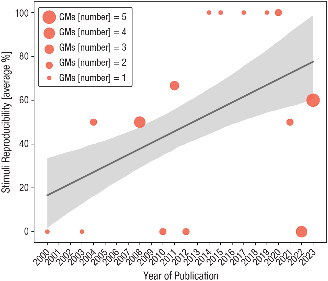
Stimuli reproducibility throughout the years. The figure depicts the average proportion of GMs that provided stimuli reproducibility (y-axis) as a function of the GMs’ publication year (x-axis). Stimuli reproducibility has constantly grown over the years. Orange circles depict GMs, and their size changes according to the number of GMs published in the same year. For example, four GMs were published in 2022 and five in 2023. Correspondingly, the circle representing GMs from 2023 will be larger and more transparent than the circle representing the GMs published in 2022. As the publication year progressed, so did the proportion of GMs that provided stimuli reproducibility, r(15) = .453, 95% CI = [.014, 1], p = .045, with weak to moderate Bayesian evidence supporting this effect, BF₁₀ = 2.25. The black line denotes the linear regression fit line, and the standard deviation is represented by the shaded gray curve. GMs = generation methods to generate non symbolic numerical stimuli; CI = confidence interval.

Controlled properties

Low to medium similarity in some controlled properties, with most GMs controlling total surface area

The different methods controlled for 16 properties (see Fig. 5). Properties were categorized into intrinsic properties, defined at the level of individual items, or extrinsic properties, defined according to the relationships between items of the whole array. Figure 9 displays the relative frequency of GMs that controlled specific properties. The average relative frequency of all controlled properties was approximately 22%, SEM = 5.648.

Fig. 9.

The relative frequency of the controlled properties. The figure depicts the distribution of different controlled properties. No property was controlled for by all GMs, but the total surface area was controlled for by most of the GMs. Half of the properties were controlled for by only one or two of the GMs. Intrinsic properties were more frequently controlled for than extrinsic properties. The list of properties is presented on the x-axis. Bars represent the relative frequency of the controlled properties between the GMs. The controlled properties were grouped into intrinsic and extrinsic properties and are marked in blue and red, respectively. The properties within the intrinsic and extrinsic groups were ordered from the most frequently controlled property to the least frequently controlled property. When two properties were equally controlled by the GMs, they were ordered in the figure according to the order provided in Figure 5. GMs = generation methods to generate non symbolic numerical stimuli.

No single property was controlled by all methods. Yet some properties were controlled for by a high portion of GMs. The two most controlled-for properties were intrinsic properties—total surface area and average surface area were controlled for in ≈81% and ≈53% of the methods, respectively. Examining the union and intersection of the GMs that controlled for the total surface area and items’ surface area or only one of these properties shows that 44% of the GMs controlled for both properties and that 91% controlled for at least one of them. Therefore, there is a medium similarity in the controlled-for intrinsic properties. The most frequently controlled extrinsic properties were density and convex hull area, controlled in ≈38% of the methods. Only 19% of the methods controlled both the items’ density and convex hull, and 56% of the methods controlled at least one of these properties. Therefore, there is a low to medium similarity among GMs in the controlled extrinsic properties.

High diversity in the controlled properties

Our findings showed that no single property was controlled for by all methods. Instead, either the total surface area or average surface area were controlled in the majority of GMs. Following these findings, we wanted to quantify how diverse GMs’ choices of controlled-for properties were. To test the diversity in the GMs’ controlled properties, we measured the asymmetry of the GMs’ controlled-properties distribution by calculating skewness (Groeneveld & Meeden, 1984; MacGillivray, 1986; Pearson, 1895). Physical properties are categorial discrete variables, and skewness is regularly defined for continuous variables. However, because our data do not refute the assumptions about the skewness of categorial variables (Klein & Doll, 2021), we used the general skewness formula. The controlled-properties distribution had a medium to high positive skewness of 1.353, SE = 0.564. Therefore, although either total or average surface area was controlled for by most GMs, the remaining properties had a low probability a GM would control them. The medium to high skewness also indicates that GMs’ choices of controlled properties were not evenly spread. Finally, there was also a high diversity in the controlled properties, diversity index = .882. Diversity was calculated using the Gini-Simpson’s index of diversity usually denoted using D or G but here for clarity was denoted using the notation “diversity index” (Keylock, 2005; Lande, 1996; Simpson, 1949; Tran et al., 2021). Here, diversity index measures the probability that two GMs will control for different properties. The higher the diversity index is, the higher the probability that the two compared GMs will control different properties. Therefore, there was a high probability that different GMs would control for different properties.

Most GMs controlled a few properties but were diverse in the number of controlled properties

The total number of types of properties controlled in all GMs was 16 (see Fig. 5). However, each GM had actually controlled for a much lower number of properties, M = 3.5, SEM = 0.291. Approximately 59% of the methods controlled for two to three properties. In contrast to the low number of properties controlled by a large portion of GMs, we found that GMs were diverse in the number of controlled-for properties. The number of controlled properties ranged between one and eight. The distribution of the number of controlled properties was not evenly distributed because more than half of the GMs controlled for two or three properties (respectively, 10 and nine GMs). Furthermore, there was a high diversity in the number of properties controlled by the GMs, with diversity index = .798. Therefore, there was a high probability that different GMs would control a different number of properties.

Control for intrinsic properties was more common

GMs controlled for two categories of properties consisting of seven intrinsic and nine extrinsic properties (see section Controlled Properties). Figure 10 displays the relative properties of GMs’ choices to control a certain category or both categories. A majority of 63% of the methods controlled for both intrinsic and extrinsic properties, whereas 34% of the methods controlled for only intrinsic properties, and the remaining ≈3%, equivalent to one GM (Dakin et al., 2011), controlled for only extrinsic properties. The average number of intrinsic properties controlled by the GMs (M = 2.25, SEM = 0.191) was higher than the number of extrinsic properties controlled by the GMs (M = 1.25, SEM = 0.196). According to the ratio of the average number of extrinsic-intrinsic properties, GMs chose to control 80% more intrinsic than extrinsic properties. We calculated the normalized average of controlled intrinsic properties, M = 1.75, SEM = 0.148, considering that there were more extrinsic than intrinsic properties (intrinsic: N = 7; extrinsic: N = 9), and still, the number of intrinsic properties was higher by the GMs than the number of extrinsic properties. There was medium to high diversity in the control of intrinsic and extrinsic properties, but they were equally diverse, with an equal diversity index of .754 for both categories. Because both types of properties’ diversity indexes were equally high, there was a high and independent equal probability that two GMs would control a different number of intrinsic or extrinsic properties. The diversity result marks the high diversity between GMs and the diversity in the control of different types of intrinsic and extrinsic properties.

Fig. 10.

The relative frequency of the controlled properties categories. The figure depicts the distribution of different controlled properties categories. Most GMs controlled for only intrinsic properties. The list of properties categories is presented on the x-axis, and the bars represent the between-GMs relative frequency. GMs = generation methods to generate non symbolic numerical stimuli.

Over the years, the types of controlled properties increased, but individual GMs’ control did not

In each year, different properties were controlled by different GMs, increasing the total number of types of properties controlled by all GMs. As shown in Figure 11, throughout the years, the sum of available controlled properties has constantly increased. Publication year explains 92.8% of the variance in the sum of available controlled properties, F(1, 30) = 388.694, p < .001, r(32) = .963, 95% CI = [.926, .982], with decisive Bayesian evidence supporting this effect, BF₁₀ > 1,000. Inspecting the regression model coefficients reveals that every GM publication added almost half of a property to the pool of available properties, Predicted Number of Available Properties = 0.468 × Actual Number of Available Properties – 931.464. In contrast, the number of properties actually controlled for by the individual GMs did not increase across the years and in some years, even decreased. Publication year did not explain the number of controlled properties, r(32) = –.242, 95% CI = [–.544, 0.117], p = .183, with weak Bayesian evidence supporting the null effect, BF₀₁ = 1.471. Analyzing the same analysis of the change in the number of controlled properties across years but looking separately at intrinsic and extrinsic categories does not provide different evidence. The number of intrinsic and extrinsic properties that were actually controlled for by the GMs did not significantly increase across the years, with weak to moderate Bayesian support for null effects, intrinsic: r(32) = –.203, p = .264, BF₀₁ = 2.503; extrinsic: r(32) = –.161, p = .378, BF₀₁ = 3.135. Furthermore, the diversity in the number of properties controlled by the GMs has changed throughout the years but in relatively small proportions. According to a comparison of diversity index of the number of controlled properties before and after 2011, the probability that two GMs would control a different number of properties had increased by only ≈4% after 2011. Importantly, we do not imply that controlling more properties is necessarily better. Instead, we wanted to provide information on the state of the field in terms of the number of controlled properties. The increase in the total number of properties available for control indicates that new ideas were introduced to the field. The stability in the number of properties controlled by the GMs indicates that new ideas were not easily implemented.

Fig. 11.

Individual GMs’ number of controlled properties compared with the total number of properties available for control across the years. (Left) The number of properties that individual GMs actually controlled for as a function of the year in which the GMs were published (x-axis). (Right) The total number of properties available for control also as a function publication year. Across the years, the total number of properties available for control for all GMs has constantly grown, whereas the number of properties actually controlled by individual GMs has not. Circles denote GMs. The purple color represents the number of properties actually controlled for by the GMs, and the light-blue color represents the total number of available properties. The size of the circles changes as a function of the number of GMs published in the same year that had the same value of properties. For example, in 2022, four GMs were published. This is represented on the left by two purple circles in different sizes. Three GMs controlled for two properties, and one controlled for a single property. Therefore, the GMs were plotted as separate purple circles. The three GMs circle size is larger than the circle of the single GM controlling for a single property. In addition, all GMs published in 2022 could control for 14 different available properties, therefore the four GMs were plotted as a single large light-blue circle. Linear correlation shows that as publication year progressed, so did the number of available properties, r(32) = .963, 95% CI = [.926, .982], p < .001, with decisive Bayesian evidence supporting this effect, BF₁₀ > 1,000. In contrast, publication year has not explained the number of controlled properties, r(32) = –.242, 95% CI = [–.544, .117], p = .183, with weak to moderate Bayesian evidence supporting the null effect, BF₀₁ = 1.944. The black line denotes the linear regression fit line, and the standard deviation is represented by the shaded gray curve. GMs = generation methods to generate non symbolic numerical stimuli; CI = confidence interval. See the full-text version for a full-scale view of Figure 11.

Controlled types

More than half of the GMs used congruency, saliency, and sizes heterogeneity within as control types

Five different control types were used (see Fig. 4). The relative frequency of the methods that used various control types is displayed in Figure 12. No single control type was used by all methods. The average relative frequency of the different control types was equal to approximately 40%, SEM = 10.505, equivalent to approximately two controls per GMs. Importantly, 53% to 62% of GMs used the same three control types: congruency, saliency, and sizes heterogeneity within. Approximately 62% of the GMs used congruency, 56% used saliency, and 53% used sizes heterogeneity within. Note that ≈84% of the methods used at least one of these control types, and 55% of the methods used at least one combination of these control types. Therefore, there is a high similarity in the control types used by the different methods. However, in general, the chance that two GMs would use different control types was approximately 75%, with a medium to high diversity index = .758. Therefore, although there were more common control types, GMs diverged in the control types they chose.

Fig. 12.

GMs’ use of various control types. The figure depicts the relative frequency of use of different control types by the different GMs. Approximately 84% of the GMs used at least one of these control types: congruency, saliency, and sizes heterogeneity within. The x-axis presents the list of control types. The y-axis presents the relative frequency of the GMs that used these control types. The control types are ordered from the most frequently used to the least frequently used control type. GMs = generation methods to generate non symbolic numerical stimuli.

GMs employ a stable number of control types throughout the years

Using a nondirectional test, we found that throughout the years, the average number of control types employed by GMs has not significantly changed, r(32) = –.289, 95% CI = [–0.579, 0.066], p = .109, without enough Bayesian support for a null effect, BF₀₁ = 1.327. To provide a more nuanced analysis, we compared different time periods before and after 2011, which marks half of the reviewed time period. We grouped the GMs into two groups, before and including 2011 and after 2011, and analyzed whether publication time was correlated with the number of control types. The difference between the average number of control types used by the GMs before and after 2011 was calculated using the Mann-Whitney U test. The Mann-Whitney U test (also known as the Wilcoxon rank sum test) is a nonparametric test for the difference between two independent samples, denoted using the statistic U (Mann & Whitney, 1947; McKnight & Najab, 2010; Wilcoxon, 1945). In general, there was no significant difference in the number of control types used by the GMs before and after 2011, U(19, 13) = 83, p = .353, r-biserial correlation = .328, with not enough Bayesian support for the null hypothesis, BF₀₁ = 0.985. In contrast, the diversity in the number of controlled types of the GMs employed increased after 2011: diversity index before 2011 = .692, diversity index after 2011 = .786. The increase in the diversity index shows that after 2011, the probability that two GMs would use a different number of control types had increased ≈14%.

Discussion

In the current review, we examined various GMs with the following objectives in mind. First, we wanted to describe the current state of the field in terms of its common language and ground. Second, we wanted to accurately map the control types and properties controlled by the different GMs. Third, we wanted to test whether the field is limited in its ability to compare between studies and to interpret results through current and new theoretical prisms. Finally, we wanted to provide guidelines for GMs. Our focus was numerical comparisons, yet our conclusions and guidelines apply to other fields and tasks involving cognitive-perceptual experiments.

Using a combination of automatic tools and human annotators who inspected the literature, we found 32 GMs (Fig. 6). These GMs used five different control types (Fig. 4) to control 16 physical properties (Fig. 5). Some of the control types can be imposed on all properties and some on only a portion of them. The control type has a low to no dependency on which properties were controlled for. Consequently, this leads to a variety of GMs and inevitably, to different stimuli sets and results (Clayton et al., 2015; DeWind & Brannon, 2016; Gebuis & Reynvoet, 2011a, 2011b; Kuzmina & Malykh, 2022; Leibovich et al., 2017; Piazza et al., 2004; Salti et al., 2017; Smets et al., 2015).

The ability to compare and replicate previous results relies on proper definitions of the controlled properties. A large portion of the GM publications lack proper definitions of properties they chose to control for. Our analysis showed that some GMs stated to control certain properties but did not define these properties. Although some of the properties do not need definitions (mainly definitions stemming from Euclidean geometry), other properties, such as density or the convex hull area, do need an exact definition. Another problem is that some of the properties were inconsistently defined between GMs (Fig. 7). Even worse, some properties were inconsistently defined within the same publication. The lack of consistency of property definitions between GMs is more harmful than the lack of definitions because it makes the GMs that have controlled for that property incomparable. Inconsistent property definitions within an article make it not only less replicable but also impossible to understand the prism through which the researchers conducted their study and the logic underlying the GM design. All in all, the lack of proper definitions creates a lack of common language, prevents proper reproduction or reanalysis of the results, and makes GMs incomparable with one another.

Designing a theory-driven GM requires providing justification for the control choices and establishing them on previous methodological prisms and numerical-cognition theories. Note that we recognized half of the GMs as non-theory-driven GMs, exhibiting very few explanatory statements for control selections. In contrast, theory-driven GMs justified controls by building on previous GMs or numerical theories and considering geometrical constraints and mathematical associations. Articulating the rationale underlying a GM’s approach to stimuli control and its implications grounds it within the context of the relevant experimental literature. More crucially, it equips fellow scientists to understand the prism through which results should be interpreted (Almaatouq et al., 2022). Finally, reflecting on the stimuli-design rationale and implications aids GM designers in interpreting their own results.

On the surface, the majority of GMs used one of a few controls. All GMs except for four controlled one of two intrinsic properties—the individual items’ surface area or the items’ total surface (Figs. 6 and 9). Note that items’ individual and total surface areas are similar properties, dependent on the radius square of the items (because most of the GMs use dot-shaped items). In addition, most GMs used the same control types (Fig. 12). Nevertheless, although most of the GMs controlled for similar properties and used similar control types, our mapping shows that the different GMs are incomparable. This is because each GM used additional controls that were highly diverse. In fact, most properties had a low probability of being controlled for. Furthermore, GMs were diverse in the total number of properties they chose to control for. Finally, the diversity of the controlled properties and control types increased throughout the years.

There is the question of whether new ideas changed the way GMs were designed. Scientific progress occurs when scientific ideas feed the scientific domain and contribute to its expansion and development (Bird, 2000; Kuhn, 1970). The numerical-cognition field is a diverse field. The diversity of the field was evident by the high variety of controlled properties and the low probability that two GMs would control for the same properties (or the same number of properties). Note that over the years, new ideas kept emerging. Accordingly, the diversity of GMs’ control choices grew during the second decade of the reviewed period. Furthermore, the number of properties available for control has constantly increased throughout the years (Fig. 11). Each new GM was predicted to add half a property to the total pool of available controls. In contrast, throughout the years, the actual number of properties GMs controlled for was stable (Fig. 11). Some properties, such as external perimeter, open space, and regularity, were suggested as being impactful in the early years of this review but were not controlled for in later years. The contrast between the increase of ideas to the stability in controlled properties suggests that the ideas coming from previous GMs are usually not adopted by later GMs. Note that the stability in controlled properties is not necessarily harmful because controlling more properties is not necessarily better. However, it provides evidence for the lack of assimilation of ideas and findings in the field.

It is worth focusing on two different properties that reflect opposing trends in the field. On one hand, the adoption of the convex hull area shows that new ideas can be successfully implemented into the field. In 2011b, Gebuis and Reynvoet showed how the convex hull area biased numerical comparisons, and since then, others have highlighted the great need to control convex hull area in numerical-comparison tasks (Clayton et al., 2015; Rodríguez & Ferreira, 2023). We found that since the convex hull area was introduced to the literature, most of the GMs have implemented it in their design. On the other hand, the case of density provides a different picture. Although a substantial portion of the GMs attempted to control density, it was not carefully defined and was therefore poorly controlled for.

The ability to reproduce, compare, and study new ideas relies on the quality and amount of shared data. In the last 2 decades, data sharing in cognitive research and other disciplines has increased (Federer et al., 2018; Kidwell et al., 2016; Martone et al., 2018; Prosser et al., 2023; Tenopir et al., 2015). Yet the shared-data quality has not necessarily increased (Tedersoo et al., 2021). GMs were inconsistent in their data-sharing practices, with different amounts, quality, and means provided for stimuli reproduction. There is evidence that stimuli reproducibility increased over the years, but it is not robust. In terms of proportion, fewer than half of the GMs provided some sort of stimuli-reproducibility method. Note that only one GM provided their actual stimuli images, complemented with results. Providing the stimuli images and details along with the data of the corresponding response would make it possible to inspect the results through the prisms of new GMs.

Taken together, the field shows a partial capability to improve GMs’ control and/or to assimilate new ideas. We think that the progress of the numerical-cognition field would be more efficient if it would be possible to compare previous ideas and test novel ideas in light of previous findings. The ability to compare ideas and test new ideas considering previous ones relies on the elaboration and precision of the method section and providing quality means for stimuli reproducibility and reanalysis.

Additional GM frameworks

We examined the broad scope of the control of physical properties. Our guiding principle was to conduct an inductive data-driven review, as opposed to a narrative-driven review. For this purpose, we used parsimonious definitions and dichotomous tagging criteria based on explicit statements. However, different GMs approach numerical cognition from various perspectives, and several of the definitions we provided could be reconsidered through other prisms. Evaluating alternative approaches and definitions is outside the scope of broadly mapping the field and providing guidelines. Yet we wanted to discuss additional nuances of stimuli control that could be considered.

We considered a GM as controlling for saliency if the veridical-mathematical ratios of two or more properties of the image arrays were matched on a decimal scale. For example, if a GM equalized the veridical ratios of the number of items and total surface area across the two presented arrays, it was tagged as controlling for saliency. Using this definition, one can study discrimination acuity by making the dimensions equally salient and consequently, equally discriminable. One example for this definition of saliency comes from Salti et al.’s (2017) GM, in which they equalized ratio with a motivation to compare the acuity of discriminating different stimuli dimensions, such as quantity and total surface area. Recently, Aulet and Lourenco (2021, 2022) suggested an alternative approach to match the perceptual rather than mathematical discriminability of quantity and surface area. In a numerical-comparison task with children (Aulet & Lourenco, 2022), when decimal-scale mathematical ratios were matched, a bias for numerosity over surface area emerged. However, when perceptual discriminability was matched, that is, ensuring changes in quantity were equally easy to discriminate as changes in total surface area, a bias for surface area over numerosity emerged. Generating a perceptually matched stimuli approach relates to long-standing debates over veridical versus nonveridical perception and appropriate methods for equating discriminability across dimensions (Akins, 1996; Hoffman, 2018; Melara & Mounts, 1993; Shepard, 1981; Wei & Stocker, 2017).

We considered a GM as controlling for saliency if it matched the ratios of two or more properties of the presented arrays. However, the statistical features of the entire stimuli set also determine saliency. Skewed, unbalanced, and highly variable distributions of stimuli properties can significantly affect results by affecting saliency across dimensions (DeWind et al., 2015; Gebuis & Reynvoet, 2011a; Park, 2022; Salti et al., 2017). We considered a GM as controlling for saliency if it matched ratios of two or more properties of the presented arrays. Different GMs with different property distributions will lead to unequal saliency, causing certain dimensions to become more perceptually prominent. For example, Park (2022) demonstrated how Yousif and Keil’s (2019) GM, by manipulating the additive area, created an unbalanced stimuli set. Specifically, the distribution of displayed quantities was much more distributed than the additive and total surface area distributions. Therefore, the item size dimension was more salient than numerosity, with much less balance in the presented quantities than in the arrays item sizes (Park, 2022). An inherent assumption of several GMs is that statistical distribution features across the entire stimuli can bias results by changing dimension saliency (DeWind et al., 2015; Gebuis & Reynvoet, 2011a; Salti et al., 2017).

Another statistical aspect of the entire stimuli set that might bias the results is the frequency of the different presented images and properties. In a recent study by Krajcsi and Kojouharova (2023), stimuli frequency affected symbolic number-comparison judgments. Participants compared numbers denoted by novel symbols with manipulated frequencies—when quantity increased, symbol frequency decreased or increased. Results showed that symbols’ frequency biased participants’ judgments (and explained the “size effect,” which is out of our scope; see Cohen Kadosh et al., 2008; Moyer & Landauer, 1967). The effect of frequency on symbolic comparisons may extend to non symbolic stimuli. More frequent stimuli could be more familiar, similar to the familiarity advantage of canonical arrangements, which exhibit grouping and/or regularity (Jansen et al., 2014; Mandler & Shebo, 1982; this mainly relates to subitizing, and there are alternative explanations relying on numerosity and not on items arrangements: Klahr, 1973; Trick & Pylyshyn, 1994). Overall, frequency effects of the entire stimuli set merit consideration in non symbolic experiments.

Often, GMs did not consider statistical aspects of the entire stimuli set. Regarding applicability, several GMs enabled control over distribution features such as ranges, variability, means, and skewness for certain properties (e.g., De Marco & Cutini, 2020; Gebuis & Reynvoet, 2011a; Piazza et al., 2004; Salti et al., 2017; Yousif & Keil, 2019; Zanon et al., 2021). However, most GMs did not provide options to control the distribution, and when available, they were for only a limited set of properties. More often, GMs reported on and/or visualized statistical distribution features (e.g., De Marco & Cutini, 2020; DeWind et al., 2015; Gebuis & Reynvoet, 2011a, 2011b; Guillaume et al., 2020; Kuzmina & Malykh, 2022; Yousif & Keil, 2019; Zanon et al., 2021). Most GMs reported only numerical ranges, with a minimal addition on physical-properties distributions. The GMs that did report on properties distributions usually reported just on range and did not provide data on the full distribution, such as the distribution mean and variability.

We tagged saliency and congruency as independent control types, based on GMs’ explicit control statements. However, saliency and congruency are not independent. Performance on non symbolic number-comparison tasks is affected by the interaction between numerical ratio, physical-property congruency, and physical-property saliency (DeWind & Brannon, 2019). Numerical ratios are the ratio between the number of items in each array. As per the canonical ratio effect, trials with lower numerical ratios approaching 1 are more difficult, and performance deteriorates (e.g., DeWind et al., 2015; Leibovich et al., 2017; Price et al., 2012). Note that performance can vastly differ between different difficult trials created by different GMs based on the congruency and saliency of the physical and numerical dimensions. Braham et al. (2018) predicted accuracy on a trial-to-trial level using stimuli generated by the Panamath GMs (Halberda et al., 2008; Halberda & Feigenson, 2008). Reynvoet et al. (2021) also generated stimuli using the Panamath GMs but also used an adapted version of the G&R GM (Gebuis & Reynvoet, 2011a). In both studies, on easy trials displaying the Panamath stimuli, accuracy was comparable regardless of physical-property congruency and saliency (Braham et al., 2018; Reynvoet et al., 2021). However, in difficult trials generated by G&R, the effects of congruity and saliency were substantially larger than for Panamath trials. In difficult G&R trials, incongruency and saliency could be associated with below-chance accuracy, whereas when using Panamath, accuracy did not decrease below 80% for all numerical ratios. Reynvoet et al. explained that physical properties in G&R stimuli were more salient than the Panamath ones because the former had more variability compared with numerical values. In convergence, DeWind et al. (2015) suggested that the effect of difficult, incongruent, and not-controlled-for saliency trials on performance is vastly different between GMs. Thus, the interaction between congruency, saliency, and numerical ratio biases results, with different GMs leading to different conclusions about numerical cognition. Note that, as reviewed in the article, understanding and comparing GMs control is often very hard.

GMs controlled for various properties over the years. However, the number of properties that can realistically be controlled in any given study is limited because there are inherent geometrical constraints and nonlinear associations between properties (e.g., De Marco & Cutini, 2020; DeWind et al., 2015; Gebuis & Reynvoet, 2011a; Piazza et al., 2002; Salti et al., 2017; see also, Shilat et al., 2021). In addition, as demonstrated earlier, GMs have many physical-property definitions that are associated with the same parameters (see Figs. 1 and 5). The interdependencies between properties restrict the number of properties GMs can control at once. The unpredictable correlations between properties restrict the number of properties that can feasibly be controlled in one study. Attempting to control too many properties would require an infeasible number of trials to counterbalance the different factors. Therefore, simply controlling more properties does not necessarily enhance methodology.

Rather than using an additive approach of controlling for more properties, GMs can account for mathematical associations in stimuli design. When done thoroughly, accounting for property associations in the design would provide better stimuli control. Several GMs have provided notable discussions of the relationships between different physical properties and incorporated these connections into their design (e.g., De Marco & Cutini, 2020; DeWind et al., 2015; Piazza et al., 2002; Salti et al., 2017). Although a full discussion of property associations is outside the scope here, properly using them can strengthen GM methodology.

One approach taken by some GMs is to group physical properties into distinct categories based on their mathematical associations. The three main GM categorizations were of (a) Piazza et al. (2004; see also Dehaene et al., 2005), (b) DeWind et al. (2015), and (c) Salti et al. (2017). These three categorizations differentiate between intrinsic properties (related to individual items) and extrinsic properties (related to the overall array). The categorized properties rely on items’ number, size, location, or a combination of the size and location. In addition, these categorizations align with the mapping to dimensions we used to analyze density’s definitions (i.e., items’ number, sizing, scattered area, and distance dimensions).

Note that the explanatory power of current intrinsic–extrinsic GMs categorization is limited. It is often difficult to compare GMs or generalize categorization with properties that were not included in the original GM. The limited explanatory power is mainly due to problematic definitions that do not enable clear category membership. Like categorization systems in other domains, the boundaries between groups can be fuzzy, and the membership to a category is not always clear (Bird & Tobin, 2018; Cole & Leide, 2006; Jacob, 2004; McCloskey & Glucksberg, 1978; Mervis & Rosch, 1981). For instance, it is not clear how to categorize properties, such as spatial frequency or luminance, that do not belong to the Euclidean domain spanning intrinsic–extrinsic dichotomy.

Nevertheless, using categorization frameworks allows GM designers to systematically consider implications of controlling certain properties over others. Relying on categorization avoids an impractical “catch-all” approach of trying to control for every possible property. Most importantly, using property categorization enables a priori postulation and prioritization of necessary experimental controls. Because categorizations are grounded in mathematical associations, they can be applied independently of the author’s assumptions about the role or bias of physical properties in numerical cognition. Ultimately, relying on property categorization enhances the explanatory power, comparability, and generalizability of GMs’ methodology and empirical findings (Almaatouq et al., 2022; Broniatowski, 2021; Makel & Plucker, 2017; Rocca & Yarkoni, 2021; Yarkoni, 2022).

We examined GMs’ control of physical properties using five identified control types. DeWind et al. (2015) introduced an alternative control approach that combines GM design with modeling. Note that this approach diverges from common control types such as congruency or saliency. Their control was reduced to systematically varying eight properties. Later, they modeled their effects on performance. The model represented physical properties and the items’ quantity across orthogonal dimensions of size, spacing, and number, which span the array’s characteristic space. This methodology of DeWind et al. is less constrained by traditional control types and avoids the impracticality of controlling numerous properties. Across the years, several GMs criticized DeWind et al.’s model and stimuli. Guillaume et al. (2020) questioned the perceptual validity of their abstract dimensions of size and spacing. Salti et al. (2017) and De Marco and Cutini (2020) pointed out that the model necessitates using homogeneous-sized items; otherwise, its dimensionality collapses. Moreover, their approach does not facilitate a detailed examination of interactions between different stimuli dimensions, such as saliency and numerical ratio, which, as we presented earlier, might produce varying effects. Fundamentally, DeWind et al.’s method deviates from other GMs, challenging our standard mapping based on tagging of control types. However, it notably pre-implements many of our subsequent recommendations (see section Conclusions and Guidelines), thereby enhancing the interpretability and comparability of the results.

The multifaced control of non symbolic numerical stimuli

In this review, we inspected the GMs from a prism of the physical properties they controlled for. The choice to focus on physical properties relies on several motivations. First, physical properties are intertwined with numerosity, and therefore, the initial control choices have major effects on the experimental results. Second, there is a wide perspective and a wealth of frameworks for controlling physical properties, whereas the need for control unifies researchers from conflicting views of numerical cognition. Third, we identified that the choice to control certain physical properties creates unique correlations between different physical properties. Such choice of control makes the stimuli in different studies incomparable. However, our focus on physical properties necessarily limited our span and created priors for the rest of the process. There are other aspects that could be considered when designing a GM, but they were not reviewed here.

Throughout this review, we considered all non symbolic numerical-comparative judgments regardless of the stimuli-presentation format. There are several presentation formats of non symbolic numerical-comparison tasks. As presented in Figure 13, the two compared arrays can be displayed simultaneously or sequentially. The two compared arrays can also be displayed in a spatially separated or spatially overlapping (i.e., intermixed) format. Studies have demonstrated discrepancies in reaction times, accuracy, and Weber fractions based on the presentation format used for the same stimuli arrays (Braham et al., 2018; Kuzmina & Malykh, 2022; Norris & Castronovo, 2016; Smets et al., 2016). Although investigating reasons for these discrepancies is outside our scope, the choice of GMs contributes to variability between presentation formats (Gilmore et al., 2011; but see Price et al., 2012). Consequently, appropriate GM selection is critical regardless of presentation type.

Fig. 13.

Two stimuli-presentation formats. The stimuli can be presented using (left) intermixed and (right) separated display modes. Arrays contain eight blue and 16 yellow dots, with a numerical ratio of 0.5. The total surface area is equal in both arrays (neutral congruency), and average surface area ratio was equated to the numerical ratio (saliency matched). Importantly, these modes of presentation exhibit different results, modulated by, among other things, control of the stimuli physical properties.

The effect and relevance of extrinsic physical properties in intermixed displays is unclear. Especially, different approaches of density would lead to different conclusions on the relationship between density and presentation format. The very influential and popular Panamath GM (Halberda et al., 2008) controlled for items’ surface area but not for extrinsic properties. Halberda et al. (2008) suggested that in intermixed displays, controlling for extrinsic properties, such as density, interdistance, and convex hull, is negligible, but they did not provide rationale for this claim. How should one consider density in an intermixed display such as shown in Figure 13? If density is calculated as the inverse of average occupancy $\frac{\mathrm{Number}}{\mathrm{Convex}\mathrm{hull}\mathrm{area}}$ , then one can ask whether the overlapping arrays share the same convex hull or have separated convex hull areas. If density is calculated as $\frac{\mathrm{Total}\mathrm{surface}\mathrm{area}}{\mathrm{Convex}\mathrm{hull}\mathrm{area}}$ , then again, how should one consider convex hull area (when total surface area is controlled for)? Considering open space in intermixed displays is also unclear. Open area is the perceived aggregated blank space not containing any items in an array. How should we consider the open space of between one of the arrays items if this space is occupied by the different array items? In contrast to the former properties relating to the item’s sizes and location, interdistance might be less problematic to consider than the former mentioned properties. Interdistance is dependent only on the items’ locations and can be calculated in one array independently of the other.

Several studies investigated the effect of extrinsic physical properties using intermixed displays. Participants were generally slower and less accurate on intermixed trials compared with spatially separated displays (Braham et al., 2018; Kuzmina & Malykh, 2022; Norris & Castronovo, 2016; Price et al., 2012). Braham et al. (2018) used Panamath and found that convex hull area and density congruency predicted accuracy, although density and convex hull were not directly controlled. Likewise, Kuzmina and Malykh (2022) tested intermixed displays. They found higher accuracy and faster responses when convex hull was incongruent with numerosity. This aligns with evidence that Panamath’s convex hull strongly correlates with numerosity (Clayton et al., 2015). Further study on the relevance of physical properties in intermixed displays is warranted. Tracking eye movements during intermixed trials may elucidate participants’ processing of extrinsic properties (Odic & Halberda, 2015). All in all, appropriately controlling physical properties remains critical across presentation formats. Different stimuli sets produce distinct correlations between numerical and physical dimensions regardless of presentation format.

Top-down strategic effects and learning effects might bias participants to attend to different physical properties according to task goals (Salti et al., 2019). Specifically, using the same stimuli but changing the task goals, such as changing the judged magnitude, influences the results. For example, changing the task from a numerical task in which the participants’ goal is to choose the more numerous array to a physical task in which the participants’ goal is to choose the larger array changes the effect of physical properties on performance (Katzin et al., 2019; Leibovich et al., 2015; Leibovich-Raveh et al., 2018; Salti et al., 2017; Tomlinson et al., 2020). Avitan et al. (2022) found that changing the task goal to choose a smaller magnitude (quantity or area) instead of the larger magnitude modulated participants’ performance and interacted with task type (numerical or physical). Leibovich-Raveh et al. (2018) manipulated participants’ emphasis on accuracy or speed during a numerical-comparison task and discovered that the effect of different physical properties was dependent on participants’ emphasis on accuracy or speed. Furthermore, the experimental block design should be considered when designing a numerical-comparison experiment. Pekár and Kinder (2020) generated their stimuli using Gebuis and Reynvoet’s (2011a) GM and found increased congruency effects when the different stimuli sets were mixed in the same block compared with blocked display of stimuli. Tokita and Ishiguchi (2010) found that the effect of physical properties was modulated by practice. Thus, different block designs and amounts of practice induce different effects and should be carefully compared with one another.

The ability to compare GMs will contribute to the understanding of symbolic numerical abilities and not only to non symbolic ones. It has been found that performance in non symbolic numerical tasks can predict a range of symbolic numerical abilities. In adults, the acuity of non symbolic comparisons is associated with age-appropriate mathematical tests, such as arithmetic tests or numerical word-problem-solving tests (e.g., Braham et al., 2018; Lourenco et al., 2012; Reynvoet et al., 2021). There is also evidence that non symbolic numerical training can include symbolic arithmetic improvements (e.g., Au et al., 2018). In children, non symbolic comparison was correlated with math achievement in childhood and adolescence (Halberda et al., 2008; Holloway & Ansari, 2009; Starr et al., 2013). Neuropsychological evidence comes from children with developmental dyscalculia showing impaired non symbolic comparisons performance (Piazza et al., 2010). Despite this body of literature, the results have been inconsistent. Several studies have suggested non symbolic comparisons are not reliable or valid measures of symbolic numerical abilities (Price et al., 2012; Sasanguie et al., 2014). It was suggested that the discrepancy between studies is the result of methodological differences and especially because of differences in the stimuli GM (Gilmore et al., 2011; Norris & Castronovo, 2016; Reynvoet et al., 2021). Reynvoet et al. (2021) found non symbolic comparison performance was related only to symbolic abilities when using Panamath stimuli (Halberda et al., 2008; Halberda & Feigenson, 2008) but not Gebuis and Reynvoet (2011a) stimuli. Therefore, GM design should also be considered when predicting symbolic numerical abilities.

The aspects mentioned above go beyond the physical properties’ consideration, demonstrating the need of choosing a prism through which GM is designed. This prism is limited because one cannot consider all aspects. Therefore, there is a need for creating a way to compare results coming from different GMS.

Conclusion and Guidelines

Taken together, the variety of different GMs, properties, and control types reflects a theoretical and methodological wealth. This wealth makes it hard to maintain a common language within the field, but its advantages are apparent. The field is thriving, given the increasing number of articles, and it has a large number of venues and ideas that could be pursued.

We see the diversity in the field as a strength and do not advocate using one GM or any other way to impose a common language. Nonetheless, currently, it is difficult to compare GMs and results across experiments using different GMs. Accordingly, we recommend that authors provide explicit lists of controlled properties and control types, preferably using common terminology from the literature. Clear, consistent verbal and mathematical definitions should be supplied for all controlled properties and control types. These definitions should encompass all study properties of interest—including uncontrolled ones—relating to hypotheses, conclusions, or known biases of interest. Articulating control statements and definitions in this manner enhances comparability, replicability, interpretability, and explanatory power, making previous ideas translatable in light of newer views (Almaatouq et al., 2022; Broniatowski, 2021; Makel & Plucker, 2017; Rocca & Yarkoni, 2021; Yarkoni, 2022).

We recommend GM designers contemplate their own control choices and consider their implications. Furthermore, GMs should also provide explicit justifications for control choices grounded in prior literature and theory and discuss the implications of those control decisions. A solid and comprehensive foundation offers several advantages: (a) It serves as a bridge between theory and methodology, (b) it provides a prism through which results are interpreted, (c) it allows considering theoretical and methodological trade-offs, (d) it enhances GMs’ comparability by providing principles for comparing between GMs, and (e) it enhances GMs’ generalizability, mainly by allowing the reconciliation of novel ideas within the context of previous GMs.

We recommend providing access to the code package used to generate the stimuli. Providing access to the original code will allow more careful understanding of property calculations and control type logic. In addition, the control of some properties requires imposing numerous constraints on the stimuli, and providing the code will aid in understanding them. Finally, providing the code will allow testing of further questions and issues not tested in the original work.

The inherent associations between physical properties restrict the number that can feasibly be controlled in one study. However, property associations can inform control choices. We recommend authors consider the mathematical associations between their properties of interest a priori. Properties differ in independence given associations with other properties. A priori analysis of mathematical associations enables prioritizing properties of greater independence or relevance while accounting for realistic constraints on simultaneous control in one study. The literature offers some notable discussions of property associations (e.g., De Marco & Cutini, 2020; DeWind et al., 2015; Piazza et al., 2002; Salti et al., 2017).

Controlling some properties places numerous constraints on stimuli. Given complex intercorrelations, predicting all impacts is challenging, and it is very hard to predict how controlling one or more properties might affect other properties. Accordingly, we suggest that authors should perform postproduction analysis and examine the correlations among the different properties after the stimuli are produced. Postproduction analysis would permit understanding of how the property associations are realized in the actual stimuli. It can measure multicollinearity and other factors that can bias conclusions. Most critically, it allows evaluating whether the design and the results interpretations align with hypotheses, establishing result validity.

We suggest GM designers consider and provide comprehensive details on control distributions because full stimuli-set statistics can bias results. Alongside numerical ranges, report at least one central tendency and dispersion measure of the controls. For asymmetric distributions, include at least two central tendency measures. If applicable, state the sampling distribution used. Provide not only summaries per array but also characterize overall set properties across arrays. Thorough distribution reporting of both GM designers themselves and fellow researchers would allow for assessing possible confounds and effects from variability, skewness, and so on.

In addition, we strongly recommend providing the actual stimuli image files, even if generated procedurally. Stimuli should be paired with behavioral- and neural-response data (where applicable) for each trial. This way, new ideas could be tested by reanalyzing previous studies (e.g., Shilat et al., 2021). Moreover, supplying stimuli with responses allows extracting and examining statistical image features and correlations post hoc—yielding insights even if such data were not originally documented. Overall, releasing full stimulus sets and trial-level responses significantly enhances replicability, analytical flexibility, interpretability, and potential cumulative knowledge growth.

These recommendations are in line with open-source practices, which increase study reliability and provide community-based knowledge sharing (AlMarzouq et al., 2005; Makel & Plucker, 2017). Hopefully, these recommendations will enable researchers to better understand results obtained using different methods and provide more generalizability and reproducibility to the field (Almaatouq et al., 2022; Broniatowski, 2021; Makel & Plucker, 2017; Rocca & Yarkoni, 2021; Schooler, 2014). These recommendations allow diversity on one hand and an ability to examine old data through new prisms on the other hand. Suggested guidelines for GMs appear in Box 1. These guidelines provide a framework for stimuli control and can be implemented in other cognitive-research domains involving perceptual decisions.

Box 1.

Guidelines

1. Provide control statements Provide an explicit list of all controlled properties and control types. 2. Provide control definitions Provide a list of explicit and consistent verbal and mathematical definitions. 3. Consider and provide justifications and implications Consider and provide grounded justifications for the control choices and discuss their implications. 4. Provide stimuli-generation code Provide the code package used to generate the stimuli. 5. Consider associations Consider property associations when choosing controls. 6. Perform postproduction analysis Examine the correlations among different properties after producing the stimuli. 7. Consider and report stimuli distribution Consider the stimuli distribution and provide comprehensive details on distributions, which allows assessing possible confounds and effects. 8. Provide stimuli and responses Provide the actual stimuli images alongside the corresponding responses to each stimulus.