Sage Journals: Discover world-class research

Abstract

Meta-analysis is a statistical technique that combines the results of multiple studies to arrive at a more robust and reliable estimate of an overall effect or estimate of the true effect. Within the context of experimental study designs, standard meta-analyses generally use between-groups differences at a single time point. This approach fails to adequately account for preexisting differences that are likely to threaten causal inference. Meta-analyses that take into account the repeated-measures nature of these data are uncommon, and so this article serves as an instructive methodology for increasing the precision of meta-analyses by attempting to estimate the repeated-measures effect sizes, with particular focus on contexts with two time points and two groups (a between-groups pretest–posttest design)—a common scenario for clinical trials and experiments. In this article, we summarize the concept of a between-groups pretest–posttest meta-analysis and its applications. We then explain the basic steps involved in conducting this meta-analysis, including the extraction of data and several alternative approaches for the calculation of effect sizes. We also highlight the importance of considering the presence of within-subjects correlations when conducting this form of meta-analysis.

Keywords

meta-analysis repeated-measures pretest–posttest design mixed-design clustered analysis

Meta-analyses allow researchers to combine multiple studies to address some research question more definitively, such as whether an intervention shows promise for reducing the symptoms of some disease or whether alternative advertising campaigns result in greater sales. In intervention and prevention sciences, meta-analyses are frequently used to pool randomized controlled trials (RCTs), but standard meta-analyses typically require researchers to perform simple comparisons of either two between-groups scores or the within-groups change. In repeated-measures designs in which multiple measurements are clustered “within” a participant (i.e., one participant is measured on some outcome more than once), the variance within these clusters is expected to be lower than variance between other participants. Under maximum likelihood and least squares regression estimation (among others), such an imbalance typically leads to overestimation of effect sizes and increased Type I error rates (Dalmaijer et al., 2022). Indeed, the Cochrane training handbook warns prospective meta-analysts to be cautious about including repeated measurements of participants without sufficient safeguarding against unit-of-analysis errors (Higgins et al., 2019a).

Researchers will often avoid clustered outcome analyses in favor of a single between-groups comparison (in RCTs, most often the between-groups difference at some postintervention follow-up) or report both between- and within-subjects outcomes as separate analyses and attempt to reconcile the effects. Neither approach is wholly satisfactory because unadjusted within-subjects analysis can lead to overestimation, and postintervention between-groups differences in means are unreliable when preintervention differences exist. For example, an intervention may successfully halve the severity of a disease’s symptoms after intervention, but if the participants who received such an intervention started with symptoms twice as severe as control participants, no between-groups effect will be detected. Although the random assignment of participants mitigates the influence of preintervention differences on postintervention outcome scores, this method is rarely entirely effective (especially in smaller or pilot studies, which renders emergent fields as particularly vulnerable; Wadhwa & Cook, 2019) and results in misestimation of effect sizes. Because meta-analysis pools the results of RCTs, these errors are then pooled with them and potentially compounded. The risk is not entirely reduced in larger RCTs, either. Sole focus on differences at postintervention can also lead to ambiguous conclusions because a postintervention difference could reflect (a) stability in the intervention group relative to deterioration in the control group, (b) improvement in the intervention group relative to stability in the control group, or (c) some combination of the two. Within-groups effects better contextualize the difference observed at postintervention and can help differentiate an intervention that prevents further symptom worsening versus an intervention that leads to symptom improvement.

Analyses of decades of RCTs consistently identify a sizable minority of RCTs in which baseline differences exist. For example, Steeger and colleagues (2021) observed that 23% of 851 reviewed RCTs reported more than one significant baseline difference between experimental and control conditions. Three decades earlier, Altman and Dore (1990) observed comparable proportions of baseline nonequivalence and an even higher rate of researchers failing to adjust analyses at all. Indeed, randomization is not a panacea that eliminates differences. Although demographic differences after randomization are likely benign (De Boer et al., 2015), the same cannot be said for cases in which outcome differences exist. A large trial that measures 20 demographic and outcome variables—a not unreasonable number in many fields—would be expected to report at least one significant baseline difference (for a full examination, see Altman, 1985). In sum, then, we propose that a naive calculation of between-groups meta-analysis that relies on randomization alone will be imprecise at best and misleading at worst.

A Brief Note on the Between-Groups Pretest–Posttest Design

In this article, we describe meta-analysis that combines between- and within-groups components, emphasizing what we call “between-groups pretest–posttest design,” because this design involves repeated measurements over time and a comparison between two specific groups on two occasions. For example, in environmental sciences, this could be the comparison between two competing reforestation programs to assess their effectiveness, whereas in marketing research, it might involve evaluating the impact of two different advertisement strategies on consumer behavior. Often, addressing specific research questions in this manner involves breaking down omnibus tests with more groups or time points into pairwise comparisons. For example, although repeated measures could include more elaborate combinations of groups and time points, researchers commonly emphasize comparisons between two specific groups to understand which groups differ and comparison of two different time points to understand the time frame over which this difference emerges. For this reason, we focus our current attention on between-groups pretest–posttest designs. However, when dealing with more than two time points, other approaches, such as those proposed by Feingold (2009), provide formulae for effect-size estimation in latent-growth-curve models. To contextualize our proposed meta-analytic approach, we first discuss standardizing mean differences and different approaches to measuring changes over time. From there, we provide worked examples adapted from recent meta-analysis to illustrate the application of our method.

Examination of the Standardized Mean Difference

Measurement of constructs in health and the social sciences varies considerably between studies. For example, two otherwise similar studies might use alternative measurements for depressive symptoms of differing lengths and item-response lengths—such as the depression subscale of the Depression, Anxiety, and Stress Scale (Lovibond & Lovibond, 1995), which has 14 items and four item responses, and the Montgomery-Åsberg Depression Rating Scale (Montgomery & Åsberg, 1979), which has 10 items and seven item responses. Although both scales represent valid measurements of depressive symptoms, the disparity in scale length and item response means that the two cannot be sensibly compared without converting both into a common metric. In RCTs and the meta-analysis of RCTs, researchers often prefer to report what are termed “standardized effect sizes.” Broadly, a standardized effect size is a metric that quantifies the magnitude of the treatment effect observed in individual studies, allowing for comparisons across different trials regardless of potential differences in how outcomes are measured (Ferguson, 2009).

Standardized effects fall into two categories: relative and absolute. Relative measures of effect, such as odds ratios or risk ratios, express the outcome effect as a ratio of probabilities or odds and are commonly used with nominal dependent-variable outcomes. As the name suggests, the numerical value of the relative effect is sensibly interpretable only in relation to some other value or categorization. For example, participants who receive an active treatment might be twice as likely as control participants to report a successful remission. Risk ratios calculate the ratio of the proportion of an outcome among the total number of participants within that treatment group between treatment groups. For example, in a balanced RCT with 100 participants in two conditions, one condition (A) might report 40 participants who present with an adverse outcome compared with 60 participants in the other condition (B). The absolute risk of that adverse outcome for both groups, expressed as a percentage, is 40% and 60%. Thus, the ratio of the risks is 40% divided by 60%, which means that the outcome is 66.66% as likely to occur in Condition A compared with Condition B or 33.34% less likely in Condition A compared with Condition B. Relatedly, the odds ratio takes the odds of an outcome within a condition and calculates the ratio of those odds between the conditions. In the above example, the odds of the outcome for Condition A were 40:60, or 0.67, and 60:40, or 1.5. The ratio of the two odds is 0.67 / 1.5, or 0.45. Thus, the odds of the outcome in Condition A are 45% of the odds of the outcome in Condition B.

To compare mean differences as measured by different scales or units, the standardized mean difference (SMD) is used instead. An SMD expresses the treatment effect in units of standard deviation rather than the original metric, and it is this property that is intended to allow simple comparison between studies and scales. The general form of the SMD is expressed as the difference between two average scores divided by the pooled standard deviation (Ferguson, 2009). Two of the most used SMD are Cohen’s (1970) d and Hedges’s (1981) g . The formula for the two SMDs are quite similar, differing only in the denominator of the pooled standard deviation (although, this is not always clear in the literature—other published formula for Cohen’s d also included the “–2” sample bias adjustment; Hedges & Olkin, 1985; McGrath & Meyer, 2006):

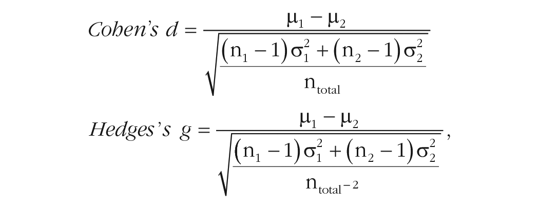
\begin{array}{l} C o h e n^{'} s d = \frac{μ_{1} - μ_{2}}{\sqrt{\frac{(n_{1} - 1) σ_{1}^{2} + (n_{2} - 1) σ_{2}^{2}}{n_{t o t a l}}}} \\ H e d g e s' s g = \frac{μ_{1} - μ_{2}}{\sqrt{\frac{(n_{1} - 1) σ_{1}^{2} + (n_{2} - 1) σ_{2}^{2}}{n_{t o t a l} - 2}}}, \end{array}

in which σ = sample standard deviation and µ = sample mean. Subscripts refer to two independent groups.

Between these two approaches, Glass’s g (alternatively called Glass’s Δ; Glass, 1976) uses the standard deviation of the control group ( $σ_{c})$ as the denominator rather than the pooled standard deviation:

Glass's g = \frac{μ_{1} - μ_{2}}{σ_{c}} .

Glass’s use of the control-group standard deviation follows from the assumption that the control group represents the baseline measure that an intervention is intended to differ from and that the variance is equal to the variance of an active intervention. However, in practice and research, the latter is rarely true—designs that might begin as balanced typically atrophy until they are not. Hedges and Olkin (1985) were among the first to demonstrate that Glass’s g was outperformed by other SMDs but were also able to establish that as sample size increases, the difference between Cohen’s d and Hedges’s g become increasingly negligible.

Alternative SMDs for Between-Groups Pretest–Posttest Designs

Although standard SMDs are routinely used to describe between-groups differences, effect estimates that account for both between- and within-subjects differences are more complex. Morris (2008) described three different approaches based on the difference between the standardized mean change for the treatment and control groups divided by a suitable standard deviation and adjusted by a bias-correcting element. The general form of the effect (called “PPC” for pretest–posttest-control) is familiar:

P P C = \frac{(μ_{E p o s t} - μ_{E p r e}) - (μ_{C p o s t} - μ_{C p r e})}{σ},

in which the numerator is the difference of the change in mean scores between experimental (E) and control (C) conditions.

The three alternative effect sizes differ (primarily) according to how the standard deviation in the denominator is calculated, either (a) calculating the pretest standard deviation separately for the experimental and control conditions (Becker, 1988; later corrected in Morris, 2000), (b) pooling the pretest standard deviations for both experimental and control conditions (Carlson & Schmidt, 1999), or (c) pooling the pre- and posttest standard deviations across both conditions (Dunlap et al., 1996; Taylor & White, 1992).

The latter two effects represent attempts to overcome statistical inefficiencies in Becker’s (1988) work—predominantly, that the assumption that the standard deviations are homogeneous between groups should allow researchers to pool them and increase precision. The SMD effect sizes proposed by Carlson and Schmidt (1999) and Dunlap et al. (1996) differ according to how posttest variance is used. Carlson and Schmidt observed that the estimated effect size can be inflated because of likely heterogeneous posttest variance, that is, the combination of intervention effects and attrition tend to inflate the variance of outcomes compared with pretest measures. Earlier, Dunlap et al., observed that the correlation between repeated measurements strongly influenced both the precision and size of the estimate—strong correlations between pretest and posttest measures will yield smaller error terms and greater statistical significance, whereas failing to account for the correlation in measures will result in an overestimated effect.

A close comparison of all three measures by Morris (2008) suggested that all three methods provide generally similar results, although Carlson and Schmidt’s (1999) method appeared least influenced by biased estimates and smaller samples. Carlson and Schmidt’s approach may be more appropriate in contexts in which heterogeneity in postintervention variance is more pronounced. Even so, each of these approaches is insensitive to potential mean differences at baseline and may thus provide an incomplete picture of level and direction of change attributable to the intervention.

Our Proposal

Selection of a suitable effect size to meta-analyze from between-groups pretest–posttest designs for RCTs is complicated and can be computationally complex without clear, practical benefit to a researcher or clinician (see e.g., Lin & Aloe, 2021). Although the relative impact of one SMD approach over another can at times be quite small (e.g., those detailed in Morris, 2008), awareness of alternative approaches and their suitability across different contexts can be beneficial for researchers. There is need to understand and articulate assumptions underlying one’s choice of method, including consideration of the plausibility of these assumptions for these data.

We propose an alternative to Morris’s (2008) three approaches, which seeks to explicitly account for differences in group means over time and within-subjects variance when investigating causal inference in between-groups pretest–posttest designs. Here, we demonstrate the utility of this meta-analysis approach using both pre- and postintervention standard deviations to calculate the standard deviation of the change, coupled with mean difference scores. Such an approach has numerous desirable qualities, including (a) accounting for the correlation between measurements over time, (b) maintaining independence of standard deviations between groups, (c) being a computationally straightforward approach that can be informed by researcher estimates, and (d) having easy calculations for use in most meta-analysis software packages.

As we elaborate shortly, neither the Morris (2008) approaches nor this alternative method are necessarily better across all research contexts. The PPC effect sizes, for instance, may not fully account for differences at baseline in means, and the two computable approaches might overlook the subtleties in postintervention heterogeneity in variance. Although our approach strives to address these concerns, it is also not without its own imperfections. Primarily, the necessity to estimate correlations over time, a parameter rarely reported in studies, poses a challenge that is met with varying degrees of success by substituting a reliability coefficient. Given these complexities, it is useful to cultivate an awareness of these differences and to possess the capability to conduct analyses using various approaches. This versatility allows evaluation of the sensitivity of research results to underlying assumptions—a pivotal aspect of our middle-ground solution, one that encourages both testable and contemplative exploration.

Example: nonsignificant baseline differences at postintervention using a random-effects model

Larun et al. (2019) performed a random-effects meta-analysis for the efficacy of exercise therapy compared with treatment as usual for fatigue in chronic fatigue syndrome and calculated the postintervention fatigue scores for seven studies. The overall between-groups effect size is SMD = −0.66 (95% CI = –1.01, –0.31), favoring the exercise-therapy condition at 12 weeks, I² = 80%. We performed a recalculation based on published data from these seven RCTs (omitting combined outcomes and unpublished data). The extracted means, standard deviations, and Ns for each study at baseline and 12 weeks are shown in Table 1. To imitate the calculations of Larun et al., we used the Cochrane Collaboration’s free Review Manager software (Version 5.4; Review Manager, 2020). The default SMD used by Review Manager is Hedges’s g.

Table 1.

Extracted and Derived Descriptive Statistics for Fatigue in Randomized Controlled Trials Analyzed by Larun et al. (2019)

	Exercise						Control
	Time 1			Time 2			Time 1			Time 2
Study	M	SD	N	M	SD	N	M	SD	N	M	SD	N
Fulcher & White (1997)	28.90	7.10	33	20.5	8.90	29	30.50	5.60	33	27.4	7.40	30
Moss-Morris et al. (2005)	24.45	8.79	25	13.91	10.88	22	25.35	8.05	24	24.41	9.69	21
Powell et al. (2001)	10.20	2.60	38	4.30	5.30	38	10.60	2.08	34	10.40	2.46	34
Wallman et al. (2004)	11.60	5.01	34	8.10	4.30	29	11.40	4.34	39	9.60	4.38	29
Wearden et al. (1998)	35.90	5.11	33	30.2	7.67	33	34.00	5.43	34	32.00	5.89	34
Wearden et al. (2010)	10.49	1.12	95	8.39	3.67	85	10.34	1.17	100	9.32	3.18	92
White et al. (2011)	28.20	3.80	160	22.8	7.50	153	28.30	3.60	160	24.30	6.50	154

Table 1 presents the input exactly as entered into Review Manager, and our output is comparable to Larun et al.’s (2019); we observed a between-groups difference of SMD = −0.58, 95% CI = [–0.90, –0.26] at 12 weeks (I² = 76%). We also examined the within-groups change of the experimental (–0.92, 95% CI = [–1.07, –0.78], I² = 0%) and control conditions (–0.43, 95% CI = [–0.63, –0.23], I² = 43%). Finally, we observed negligible differences in preintervention fatigue scores (0.01, 95% CI = [–0.12, 0.15], I² = 0%). The temptation, then, is to conclude that the effect of the intervention approximates the difference in postintervention effect sizes, ≈0.92 − 0.43 = 0.49. However, this approach fails to account for the pre-post intervention correlation as an estimate of variability that might be accounted for by systematic effects (i.e., within-subjects correlations are expected to be stronger in shorter follow-ups than in longer follow-ups).

Adjustment for the Repeated Measurement in a Between-Groups Pretest–Posttest Design

To incorporate both within-groups change with between-groups differences in effect estimation for between-groups pretest–posttest designs, we calculated the effect sizes using the within-subjects mean difference and the standard deviation of the change, adjusted by a suitable estimated correlation. If estimates of correlation coefficients between measurements within a study are not readily available for meta-analysis, the test–retest reliability coefficient will suffice. For this purpose, we used the reported test–retest reliability coefficient of the Chalder Fatigue Scale, which was used for all included studies (estimated as around .58 over 10 weeks but may be even higher over shorter periods; Chilcot et al., 2016; Jelsness-Jørgensen, 2012). For simplicity’s sake, we used a single correlation estimate for all studies in the meta-analysis, although, in practice, different studies and scales will require different correlations. In meta-analysis in which different scales are pooled, the test–retest reliability coefficient should be used for each scale, and the reliability coefficient should match the pre-to-post time period as closely as possible. We note, as well, that the test–retest reliability is likely to be an overestimation and that the true correlation between measurements tends to decrease over time. Therefore, the test–retest reliability coefficient should be considered the upper limit of the correlation and used if no other information is available.

We calculated the variance of the difference according to the formula from Abrams et al. (2005), in which σ = standard deviation and ρ = the correlation between measurements. The standard deviation of the change is obtained by the square root of the resulting variance:

{σ^{2}}_{change} = σ_{p r e}^{2} + σ_{p o s t}^{2} - 2 ρ \sqrt{σ_{p r e}^{2} \times σ_{p o s t}^{2}} .

We calculated the difference in means and standard deviation of the change for each study and present the result in a forest plot (Table 2 and Fig. 1). We used the values from the first study (Fulcher & White, 1997) as our example calculation and used the 10-week test–retest reliability coefficient.

First, the average preintervention score for the exercise group was 28.9, and the average for the same group at postintervention was 20.5. Subtracting one from the other gives the difference in means (−8.4). Note that the directionality is arbitrary but must be consistent throughout all calculations (i.e., Time 1 − Time 2 or Time 2 − Time 1). Because in our example the outcome is fatigue severity, we used negative direction to indicate an improvement, that is, a reduction in fatigue. We repeated the process for the control condition (27.4 − 30.5 = −3.1).

Table 2.

Mean Differences and Standard Deviation of the Change

	Exercise		Control
Study	Mean difference	σ_change	Mean difference	σ_change
Fulcher & White (1997)	–8.40	7.50	–3.10	6.16
Moss-Morris et al. (2005)	–10.54	9.20	–0.94	8.25
Powell et al. (2001)	–5.90	4.34	–0.20	2.10
Wallman et al. (2004)	–3.50	4.31	–1.80	3.99
Wearden et al. (1998)	–5.70	6.28	–2.00	5.20
Wearden et al. (2010)	–2.10	3.15	–1.02	2.67
White et al. (2011)	–5.40	6.13	–4.00	5.29

Fig. 1.

Forest plot of adjusted between-groups pretest–posttest analysis.

Second, we then calculated the standard deviation of the change using the formula proposed by Abrams et al. (2005). The pre- and postintervention standard deviations for the experimental group are squared and summed (7.10² + 8.90² = 129.62). From this value, we subtracted the product of twice the pre-post correlation (2 × .58 = 1.16) to the square root of the product of the squared standard deviations (7.10² × 8.90² = 3,992.98; √3,992.98 = 63.19; 1.16 × 63.19 = 73.3). This second result was subtracted from the first (129.62 − 73.3 = 56.31). This is the variance of the change, and so taking the square root will provide the standard deviation (√56.31 = 7.5). The process was then repeated for the control group and, mercifully, can be expedited with simple calculators (for the R script, see the Supplemental Material available online; for the script text, see Appendix A).

Third, the resulting values were then entered into a suitable meta-analysis software package, such as Review Manager.

Observations

We first observe that the obtained between-groups pretest–posttest effect size is larger than the original estimate (SMD = −0.68, 95% CI = [–1.02, –0.35]). We also observe an increase in heterogeneity, from I² = 76% to I² = 78%. The rejection of the null hypothesis is also slightly more decisive, from an overall z score of 3.52 (p = .0004) to a z score of 3.99 (p < .0001).

Heterogeneity

Even when there is little preintervention difference between groups, the overall postintervention difference varies considerably at different correlation estimates. Such variation in postintervention effect is termed “heterogeneity,” which refers to the variability in results across studies attributable to differences in study characteristics, populations, interventions, or outcomes (Higgins et al., 2019b). Because variance is the square root of the standard deviation and the standard deviation is the denominator for the standardized effect size, it follows that the weaker the correlation is, the smaller but more homogeneous the effect size becomes. For example, if all else in the above were kept equal but the test–retest coefficient were to drop to 0.3, the effect size becomes SMD = −0.54, 95% CI = [–0.82, –0.27], I² = 69%. If the correlation (or test–retest coefficient) is increased to 0.8, the effect size becomes SMD = −0.92, 95% CI = [–1.35, –0.50], I² = 86%. In a meta-analysis in which numerous scales are combined and the test–retest reliability coefficient varies between studies, the extent of the heterogeneity will depend on the approximate average of the coefficients. Figure 2 provides a visual representation of how the effect size and heterogeneity increase according to correlation strength while the estimate’s precision decreases. We show that the effect size increases in a logarithmic fashion, as do the widths of the confidence intervals around the effect size. In contrast, we observe a linear increase in heterogeneity. The effect size approximately doubles over the period in which r = .05 and r = .8 (a wide disparity in estimated r value), but differences in effect size are more gradual in cases in which estimated and population r values differ by smaller amounts. In instances in which prior studies provide estimates of correlation, one may thus have some confidence in the r value used for calculations. In other cases, in which prior literature is unable to inform there is a wide range of possible r values to choose from, estimating effect sizes across this range may be useful for understanding robustness of an observed (pooled) effect to inaccuracies in estimating the population r value. Our provided script will be helpful for meta-analysts in this regard (see Appendix A).

Fig. 2.

Effect size, precision, and heterogeneity as correlation approaches r = 1.

Comparison with the PPC approaches outlined in Morris (2008)

For comparison’s sake, we also performed the same between-groups pretest–posttest meta-analysis using the first two adjustments proposed by Morris (2008). The third effect size proposed by Dunlap et al. (1996) is expected to have a smaller sampling distribution than the others described by Morris (2008), but no reliable method of estimating this has been produced yet. We omit the third from our comparison here for this reason. For the relevant code for replicating our findings, see the Supplemental Material; the steps for performing these analyses are broadly like the approach detailed earlier.

Several things are clear to us—each of the three approaches differ to some extent, and the two PPC approaches yield larger effect sizes with greater heterogeneity compared with the current approach (See Table 3). Although we observe larger effects using the preintervention standard deviation PPC effects, we note that these are likely to be an overestimation of the true effect of the intervention. As we show in the descriptive statistics for the extracted studies (Table 1), the standard deviations for both groups of participants tend to expand from pre- to postintervention measures. The central-limit theorem posits that scores tend to increasingly cluster around the population mean as sample sizes increase, shrinking the degree of variability. Thus, preintervention standard deviations are likely to be smaller than their postintervention counterparts as natural attrition removes participants from studies, which, in turn, shrinks the denominator used for calculating the SMD while retaining the numerator. This change in the sample sizes is not directly accounted for by PPC1 or PPC2 but is in our current approach.

Table 3.

Comparisons With Alternative SMD Calculations

	SMD	CILL	CIUL	SE	Z	p	τ²	I ²	H²
PPC1	–0.863	–1.23	–0.42	0.21	–4.00	< .001	0.238 (SE = 0.183)	81.51%	5.41
PPC2	–0.920	–1.33	–0.51	0.21	–4.38	< .001	0.261 (SE = 0.202)	88.06%	8.37
Current	–0.686	–1.02	–0.35	0.17	–3.98	< .001	0.152 (SE = 0.128)	78.01%	4.55

Note: SMD = standardized mean difference; PPC1 = pretest standard deviation separately for the experimental and control conditions; PPC2 = pooling the pretest standard deviations for both experimental and control conditions; CILL = 95% confidence interval lower limit; CIUL = 95% confidence interval upper limit.

Indeed, these examples serve to demonstrate specific circumstances in which the current approach might be a more accurate estimate of the true intervention effect: when postintervention variance differs from preintervention. Meta-analysts should be vigilant for such disparity when participant dropout is observed, especially when dropout is uneven between treatment conditions, and when heterogeneous responses are suspected. For example, a treatment condition with a smaller subset of “responders” but otherwise no attrition would likely have greater variance than another treatment condition with substantial dropout aside from a small subset for whom the intervention worked and was well tolerated. These factors (and others, such as regression to the mean) should be investigated by meta-analysts before any decision around effect-size calculation is made (see Hewitt et al., 2010; Leon et al., 2006).

Weighting in meta-analysis

Given that the proposed formula for adjusting study estimates requires adjusting the variance of the study effect sizes, examining the impact of study variance on the summary effect-size calculation in meta-analysis is useful. Studies included in meta-analyses should be weighted by the precision of their estimates. Here, we briefly show the calculations of study weight in a fixed-effects meta-analysis before generalizing to random effects. Our treatment of weighting in meta-analysis here is intended to provide context to the manner in which adjustments to effect sizes will affect the final outcome of a meta-analysis, including our adjustment to the variance of effect sizes. For a comprehensive discussion of weighting in meta-analysis, including consideration for fixed or random effects and cases in which the desired effect metric is not the mean difference between two groups, the reader is referred to the seminal work by Borenstein et al. (2010).

In fixed-effect meta-analysis, weight of a study is the inverse of the within-studies variance, given by the formulae:

\frac{σ^{2}}{n}

Fixed - effects weight (as inverse variance) = \frac{n}{σ^{2}} .

Because the numerator is the squared standard deviation, it follows that as the standard deviation increases in size, so does the variance. The same is true as N decreases. Consequently, as the variance increases in size, the study weight is penalized through the inversion. Assuming that the meta-analyst wants to estimate the mean difference between two groups as the target effect size, the summary effect size in meta-analysis is then given as the ratio of the sum of product of the study weights (w) to effect size (ES) to the sum of the study weight, or:

Summary effect size = \frac{\sum^{​} (w \times E S)}{\sum^{​} (w)} .

The precision of the estimate of the effect sizes is proportional to the weight (or inversely proportional to the precision), and so smaller, imprecise studies are de-emphasized when calculating the summary effect size. In random-effects meta-analysis, the estimate of between-studies variance (τ²) is included in the denominator of the weighting reciprocal, and so, the precision of random-effects effect sizes will always be a minimum of the fixed-effects meta-analysis.

Random-effects weight (as inverse variance) = \frac{n}{σ^{2} + τ^{2}} .

A second example: in which increased precision for within-studies estimates avoids a Type II error

We use a second example inspired by Larun and colleagues (2019), in which between-groups differences in depressive symptoms at 1 year fail to reach statistical significance; SMD = −0.32, 95% CI = [–0.82, 0.18], I² = 86%. The effect size is driven primarily by a large observed effect in favor of exercise in Powell et al. (2001); the other three studies reported null findings (Jason et al., 2007; Wearden et al., 2010) or borderline significance favoring exercise (White et al., 2011; Time 2 between-groups comparison is p ≈ .0496). However, for all studies excluding Powell et al., each exercise group started with higher mean values and ended lower—the standard between-groups comparison fails to account for the heterogeneity of change and erroneously fails to reject the null hypothesis. The extracted descriptive statistics are shown in Table 4.

Table 4.

Descriptive Statistics for 1-Year Between-Groups Comparison

	Exercise						Control
	Time 1			Time 2			Time 1			Time 2
Study	M	SD	N	M	SD	N	M	SD	N	M	SD	N
Jason et al. (2007)	21.11	11.22	21	16.94	11.82	21	17.45	6.97	24	13.50	9.97	24
Powell et al. (2001)	9.00	3.77	38	4.20	4.08	38	10.40	4.31	34	10.10	4.91	34
Wearden et al. (2010)	9.67	4.08	95	7.88	4.45	81	9.26	4.25	100	8.06	4.75	85
White et al. (2011)	8.20	3.60	160	6.10	4.10	144	8.00	3.90	160	7.20	4.70	151

Each of the four studies above used the Hospital Anxiety and Depression Scale (HADS), except for Jason et al. (2007), in which the Beck Depression Inventory-II (BDI-II) was used. The HADS has a test–retest reliability that diminishes rapidly over time from excellent over 2 weeks (r = .85), reasonable between 2 and 6 weeks (r = .75), and adequate at 6 weeks (r = .70; Herrmann, 1997). The BDI-II is similar in form, function, and test–retest reliability over the same time (r = .7; Erford et al., 2016). Given the rapid decline in test–retest reliability and the dynamic of mood measurement, it seems unlikely that the test–retest reliability would remain suitably robust for measurements made a year apart. It is also fanciful that the correlation between measurements would increase in strength, so one can reasonably assume that the true correlation is bound between a trivially weak r = .1 and the theoretical r = .7.

First, we assume the worst-case scenario, in which there is a trivially weak correlation between depressive symptoms between measurements over time. As expected, the standard deviations for each study are maximized, decreasing the overall between-studies variances and reducing the overall heterogeneity (Table 5 and Fig. 2). The smaller studies are penalized heavily, and the weight assigned to these studies is minimized. The net result is that the overall summary effect size is simultaneously the smallest of the adjusted values and also the most precise. The overall pooled effect is now SMD = −0.26, 95% CI = [–0.53, –0.00], I² = 51%. The null hypothesis is just rejected (z = 1.98, p = .048), favoring the experimental condition. As we show, when the correlation between measurements is increased, the effect size and heterogeneity increase, and the precision reduces.

Table 5.

Mean Difference and Standard Deviation of the Change Assuming a Reported Correlation of r = .1

	Exercise		Control
Study	Mean difference	σ_change	Mean difference	σ_change
Jason et al. (2007)	–4.17	15.46	–3.95	11.58
Powell et al. (2001)	–4.80	5.27	–0.3	6.2
Wearden et al. (2010)	–1.79	5.73	–1.2	6.05
White et al. (2011)	–2.10	5.18	–0.8	5.8

Next, we show the result of assuming that the observed 6-week reliability coefficient will endure for 12 months. The smaller, less precise studies are afforded slightly more influence over the summary effect through increased weights, which decreases the overall precision of the estimate while also increasing the effect size favoring the exercise condition (Table 6 and Fig. 3). Thus, there is almost certainly a Type I error. The overall effect after adjustment is SMD = −0.47, 95% CI = [–0.91, –0.03], I² = 82% (See Figure 4).

Table 6.

Mean Difference and Standard Deviation of the Change Assuming a Reported Correlation of r = .7

	Exercise		Control
Study	Mean difference	σ_change	Mean difference	σ_change
Jason et al. (2007)	–4.17	8.94	–3.95	7.12
Powell et al. (2001)	–4.80	3.05	–0.30	3.61
Wearden et al. (2010)	–1.79	3.32	–1.20	3.52
White et al. (2011)	–2.10	3.02	–0.80	3.41

Fig. 3.

Forest plot for 1-year comparison with weak correlation.

Fig. 4.

Forest plot for 1-year comparison assuming reported correlations.

A third example: a cautionary tale about the dangers of interpreting the postintervention effect without consideration of the baseline values

Finally, we finish with an example in which reliance on interpreting the overall result without carefully examining the baseline values in a between-groups pretest–posttest design leads to incorrectly rejecting the alternative hypothesis. For this purpose, we have created some sham data from our previous examples. First, we swapped the control postintervention scores for the baseline scores of the experimental condition. In this case, we see that substantial change has occurred in the control group, whereas the experimental group has remained relatively stable (Table 7; all study names removed).

Table 7.

Descriptive Statistics for the Third Example, Using Sham Data

	Time 1			Time 2					Time 1			Time 2
	Experimental			Experimental					Control			Control
	M	SD	N	M	SD	N	Mean difference	σ_change	M	SD	N	M	SD	N	Mean difference	σ_change
Study 1	28.90	7.10	33	30.50	5.60	33	1.60	5.97	20.50	8.90	29	27.40	7.4	30	6.90	7.59
Study 2	24.45	8.79	25	25.35	8.05	24	0.90	7.75	13.91	10.88	22	24.41	9.69	21	10.50	9.49
Study 3	10.20	2.60	38	10.60	2.08	34	0.40	2.19	4.30	5.30	38	10.40	2.46	34	6.10	4.36
Study 4	11.60	5.01	34	11.40	4.34	39	–0.20	4.33	8.10	4.30	29	9.60	4.38	29	1.50	3.98
Study 5	35.90	5.11	33	34.00	5.43	34	–1.90	4.84	30.2	7.67	33	32.00	5.89	34	1.80	6.41
Study 6	10.49	1.12	95	10.34	1.17	100	–0.15	1.05	8.39	3.67	85	9.32	3.18	92	0.93	3.17
Study 7	28.20	3.80	160	24.30	6.50	154	0.10	3.40	28.3	3.60	160	22.80	7.5	153	1.50	6.48

We performed the previous calculations (again using the correlation of r = .58) and obtained a moderate to large effect favoring the experimental group: SMD = −0.71, 95% CI = [–1.04, –0.38], I² = 77%. Only when we examined the descriptive statistics did we see that the effect is entirely due to the control group reporting greater fatigue over time rather than any positive influence of the experimental condition. Although lack of change in an experimental condition is not universally evidence of a null intervention (e.g., medical intervention in neurodegenerative disease would interpret long-term symptom stability in a positive manner), it further reinforces the necessity of carefully examining baseline data when interpreting results. We also see that this risk was not removed by using our technique, although our technique does make the baseline values more prominent, and the calculation of the mean difference highlights the within-studies change.

Discussion

As we have shown, the meta-analysis of between-groups pretest–posttest design data need not be limited to within-subjects or postintervention between-groups comparisons and can be extended to account for preintervention differences with minimal additional effort. Benefits of adjusted meta-analyses that account for both between-groups and within-groups components include a more valid representation of true effects, especially for cases in which baseline differences exist; improved understanding of the heterogeneity of effects that are attributable to baseline differences; and improved statistical power through the inclusion of within-studies change.

We also examined a handful of alternative approaches for calculating SMDs in between-groups pretest–posttest studies and considered the relative strengths of each. The PPC approaches detailed extensively by Morris (2008) have excellent statistical properties for studies of all sizes, particularly larger studies in which the risk of heterogeneous variances over time might be low. If heterogeneity cannot be assumed or is clearly absent, the current approach represents a viable alternative to improve the precision of summary effect sizes. Furthermore, we have shown that appropriate adjustment by the pre-post reliability coefficient allows researchers to navigate away from Type I and II errors in some plausible research scenarios. Although all meta-analysis can benefit from improved precision, early phase or small-sample research will find greatest benefit.

Given the strengths and weaknesses of the different effect-size-estimation methods tested in the present tutorial, our strongest recommendation is for authors to articulate the assumptions for the analytic approach they have chosen for effect-size estimation and the plausibility of these. In cases in which evidence for plausibility is mixed or uncertain, a combination of the demonstrated effect-size methods may provide sensitivity analyses to understand the robustness of observed effects. To facilitate straightforward investigation, our supplied code can be deployed (see Appendix A).

Supplemental Material

sj-rar-1-amp-10.1177_25152459231217238 – Supplemental material for Calculating Repeated-Measures Meta-Analytic Effects for Continuous Outcomes: A Tutorial on Pretest–Posttest-Controlled Designs

Supplemental material, sj-rar-1-amp-10.1177_25152459231217238 for Calculating Repeated-Measures Meta-Analytic Effects for Continuous Outcomes: A Tutorial on Pretest–Posttest-Controlled Designs by David R. Skvarc and Matthew Fuller-Tyszkiewicz in Advances in Methods and Practices in Psychological Science

Footnotes

Appendix A

Acknowledgements

We gratefully acknowledge the authors of our exemplar article, Lillebeth Larun, Kjetil G. Brurberg, Jan Odgaard-Jensen, and Jonathan R. Price.

Transparency

Action Editor: Yasemin Kisbu-Sakarya

Editor: David A. Sbarra

Author Contributions

David R. Skvarc: Conceptualization; Data curation; Formal analysis; Investigation; Methodology; Writing – review & editing.

Matthew Fuller-Tyszkiewicz: Formal analysis; Investigation; Methodology; Supervision; Validation; Writing – original draft; Writing – review & editing.

ORCID iD

David R. Skvarc

Supplemental Material

Additional supporting information can be found at

References

Abrams

K. R.

Gillies

C. L.

Lambert

P. C.

(2005). Meta-analysis of heterogeneously reported trials assessing change from baseline. Statistics in Medicine, 24(24), 3823–3844.

Altman

D. G.

(1985). Comparability of randomised groups. Journal of the Royal Statistical Society: Series D (The Statistician), 34(1), 125–136.

Altman

D. G.

Dore

C. J.

(1990). Randomisation and baseline comparisons in clinical trials. The Lancet, 335(8682), 149–153.

Becker

B. J.

(1988). Synthesizing standardized mean-change measures. British Journal of Mathematical and Statistical Psychology, 41(2), 257–278.

Borenstein

Hedges

L. V.

Higgins

J. P.

Rothstein

H. R.

(2010). A basic introduction to fixed-effect and random-effects models for meta-analysis. Research Synthesis Methods, 1(2), 97–111.

Carlson

K. D.

Schmidt

F. L.

(1999). Impact of experimental design on effect size: Findings from the research literature on training. Journal of Applied Psychology, 84(6), 851–862. https://doi.org/10.1037/0021-9010.84.6.851

Chilcot

Norton

Kelly

M. E.

Moss-Morris

(2016). The Chalder Fatigue Questionnaire is a valid and reliable measure of perceived fatigue severity in multiple sclerosis. Multiple Sclerosis Journal, 22(5), 677–684.

Cohen

(1970). Approximate power and sample size determination for common one-sample and two-sample hypothesis tests. Educational and Psychological Measurement, 30(4), 811–831.

Dalmaijer

E. S.

Nord

C. L.

Astle

D. E.

(2022). Statistical power for cluster analysis. BMC Bioinformatics, 23(1), Article 205. https://doi.org/10.1186/s12859-022-04675-1

10.

De Boer

M. R.

Waterlander

W. E.

Kuijper

L. D.

Steenhuis

I. H.

Twisk

J. W.

(2015). Testing for baseline differences in randomized controlled trials: An unhealthy research behavior that is hard to eradicate. International Journal of Behavioral Nutrition and Physical Activity, 12(1), 1–8.

11.

Dunlap

W. P.

Cortina

J. M.

Vaslow

J. B.

Burke

M. J.

(1996). Meta-analysis of experiments with matched groups or repeated measures designs. Psychological Methods, 1(2), 170–177.

12.

Erford

B. T.

Johnson

Bardoshi

(2016). Meta-analysis of the English version of the Beck depression inventory–second edition. Measurement and Evaluation in Counseling and Development, 49(1), 3–33.

13.

Feingold

(2009). Effect sizes for growth-modeling analysis for controlled clinical trials in the same metric as for classical analysis. Psychological Methods, 14(1), 43–53.

14.

Ferguson

C. J.

(2009). An effect size primer: A guide for clinicians and researchers. Professional Psychology: Research and Practice, 40(5), 532–538.

15.

Fulcher

K. Y.

White

P. D.

(1997). Randomised controlled trial of graded exercise in patients with the chronic fatigue syndrome. BMJ, 314(7095), 1647–1652. https://doi.org/10.1136/bmj.314.7095.1647

16.

Glass

G. V.

(1976). Primary, secondary, and meta-analysis of research. Educational Researcher, 5(10), 3–8.

17.

Hedges

L. V.

(1981). Distribution theory for Glass’s estimator of effect size and related estimators. Journal of Educational Statistics, 6(2), 107–128.

18.

Hedges

L. V.

Olkin

(1985). Statistical methods for meta-analysis. Academic Press.

19.

Herrmann

(1997). International experiences with the Hospital Anxiety and Depression Scale: A review of validation data and clinical results. Journal of Psychosomatic Research, 42(1), 17–41.

20.

Hewitt

C. E.

Kumaravel

Dumville

J. C.

Torgerson

D. J.

, & Trial Attrition Study Group. (2010). Assessing the impact of attrition in randomized controlled trials. Journal of Clinical Epidemiology, 63(11), 1264–1270.

21.

Higgins

J. P.

Deeks

J. J.

(2019a). Choosing effect measures and computing estimates of effect. In Higgins

J. P. T.

Thomas

Chandler

Cumpston

Page

M. J.

Welch

V. A.

(Eds.), Cochrane handbook for systematic reviews of interventions (pp. 143–176).

22.

Higgins

J. P.

Deeks

J. J.

(2019b). What is heterogeneity? In Higgins

J. P. T.

Thomas

Chandler

Cumpston

Page

M. J.

Welch

V. A.

(Eds.), Cochrane handbook for systematic reviews of interventions.

23.

Jason

L. A.

Torres-Harding

Friedberg

Corradi

Njoku

M. G.

Donalek

Reynolds

Brown

Weitner

B. B.

Rademaker

Papernik

(2007). Non-pharmacologic interventions for CFS: A randomised trial. Journal of Clinical Psychology in Medical Settings, 14(4), 275–296. https://doi.org/10.1007/s10880-007-9090-7

24.

Jelsness-Jørgensen

L. P.

(2012). The Fatigue Questionnaire has a good test-retest profile in IBD. Alimentary Pharmacology & Therapeutics, 35(5), 621–622.

25.

Larun

Brurberg

K. G.

Odgaard-Jensen

Price

J. R.

(2019). Exercise therapy for chronic fatigue syndrome. Cochrane Database of Systematic Reviews. https://doi.org/10.1002/14651858.CD003200.pub7

26.

Leon

A. C.

Mallinckrodt

C. H.

Chuang-Stein

Archibald

D. G.

Archer

G. E.

Chartier

(2006). Attrition in randomized controlled clinical trials: Methodological issues in psychopharmacology. Biological Psychiatry, 59(11), 1001–1005.

27.

Lin

Aloe

A. M.

(2021). Evaluation of various estimators for standardized mean difference in meta-analysis. Statistics in Medicine, 40(2), 403–426.

28.

Lovibond

S. H.

Lovibond

P. F.

(1995). Manual for the depression anxiety stress scales (2nd ed.). Psychology Foundation.

29.

McGrath

R. E.

Meyer

G. J.

(2006). When effect sizes disagree: The case of r and d. Psychological Methods, 11(4), 386–401. https://doi.org/10.1037/1082-989X.11.4.386

30.

Montgomery

S. A.

Åsberg

(1979). A new depression scale designed to be sensitive to change. The British Journal of Psychiatry, 134(4), 382–389.

31.

Morris

S. B.

(2000). Distribution of the standardized mean change effect size for meta-analysis on repeated measures. British Journal of Mathematical and Statistical Psychology, 53(1), 17–29.

32.

Morris

S. B.

(2008). Estimating effect sizes from pretest-posttest-control group designs. Organizational Research Methods, 11(2), 364–386.

33.

Moss-Morris

Sharon

Tobin

Baldi

J. C.

(2005). A randomised controlled graded exercise trial for chronic fatigue syndrome: Outcomes and mechanisms of change. Journal of Health Psychology, 10(2), 245–259.

34.

Powell

Bentall

R. P.

Nye

F. J.

Edwards

R. H.

(2001). Randomised controlled trial of patient education to encourage graded exercise in chronic fatigue syndrome. BMJ, 322(7283), 387–390. https://doi.org/10.1136/bmj.322.7283.387

35.

Review Manager (RevMan) (Version 5.4) [Computer program]. (2020). The Cochrane Collaboration.

36.

Steeger

C. M.

Buckley

P. R.

Pampel

F. C.

Gust

C. J.

Hill

K. G.

(2021). Common methodological problems in randomised controlled trials of preventive interventions. Prevention Science, 22(8), 1159–1172.

37.

Taylor

M. J.

White

K. R.

(1992). An evaluation of alternative methods for computing standardized mean difference effect size. The Journal of Experimental Education, 61(1), 63–72.

38.

Wadhwa

Cook

T. D.

(2019). The set of assumptions randomised control trials make and their implications for the role of such experiments in evidence-based child and adolescent development research. New Directions for Child and Adolescent Development, 2019(167), 17–37.

39.

Wallman

K. E.

Morton

A. R.

Goodman

Grove

Guilfoyle

A. M.

(2004). Randomised controlled trial of graded exercise in chronic fatigue syndrome. Medical Journal of Australia, 180(9), 444–448.

40.

Wearden

A. J.

Dowrick

Chew-Graham

Bentall

R. P.

Morriss

R. K.

Peters

Riste

Richardson

Lovell

Dunn

, & Fatigue Intervention by Nurses Evaluation (FINE) Trial Writing Group and the FINE Trial Group. (2010). Nurse led, home based self help treatment for patients in primary care with chronic fatigue syndrome: Randomised controlled trial. BMJ, 340, Article c1777. https://doi.org/10.1136/bmj.c1777

41.

Wearden

A. J.

Morriss

R. K.

Mullis

Strickland

P. L.

Pearson

D. J.

Appleby

Campbell

I. T.

Morris

J. A.

(1998). Randomised, double-blind, placebo-controlled treatment trial of fluoxetine and graded exercise for chronic fatigue syndrome. The British Journal of Psychiatry, 172(6), 485–490. https://doi.org/10.1192/bjp.172.6.485

42.

White

P. D.

Goldsmith

K. A.

Johnson

A. L.

Potts

Walwyn

DeCesare

J. C.

Baber

H. L.

Burgess

Clark

L. V.

Cox

D. L.

Bavinton

Angus

B. J.

Murphy

O’Dowd

Wilks

McCrone

Chalder

Sharpe

, & PACE Trial Management Group. (2011). Comparison of adaptive pacing therapy, cognitive behaviour therapy, graded exercise therapy, and specialist medical care for chronic fatigue syndrome (PACE): A randomised trial. The Lancet, 377(9768), 823–836. https://doi.org/10.1016/S0140-6736(11)60096-2

Supplementary Material

Please find the following supplemental material available below.

For Open Access articles published under a Creative Commons License, all supplemental material carries the same license as the article it is associated with.

For non-Open Access articles published, all supplemental material carries a non-exclusive license, and permission requests for re-use of supplemental material or any part of supplemental material shall be sent directly to the copyright owner as specified in the copyright notice associated with the article.

0.00 MB