Interacting With Curves: How to Validly Test and Probe Interactions in the Real (Nonlinear) World

Abstract

Hypotheses involving interactions in which one variable modifies the association between another two are very common. They are typically tested relying on models that assume effects are linear, for example, with a regression like y = a + bx + cz + dx × z. In the real world, however, few effects are linear, invalidating inferences about interactions. For instance, in realistic situations, the false-positive rate can be 100% for detecting an interaction, and a probed interaction can reliably produce estimated effects of the wrong sign. In this article, I propose a revised toolbox for studying interactions in a curvilinear-robust manner, giving correct answers “even” when effects are not linear. It is applicable to most study designs and produces results that are analogous to those of current—often invalid—practices. The presentation combines statistical intuition, demonstrations with published results, and simulations.

Studying interactions in which a variable moderates the relationship between two other variables is common in psychology. For instance, 71% of articles in the March 2020 issues of Journal of Personality and Social Psychology, Journal of Experimental Psychology: General, and Psychological Science tested for interactions. The general approach to studying interactions is the same for the majority of statistical models commonly used by social scientists (e.g., linear and logit regression, multilevel models, structural equation modeling), and it consists of three steps. For concreteness, I discuss them relying on a stylized scenario in which one wishes to examine the interaction between the effects of age and gender on people’s weight. In the first step, one estimates a model that imposes the assumption that all predictors (including possibly nonlinear terms) and including the interaction have linear associations with the (latent, if applicable) dependent variable. ¹ For example, in the first step, one estimates the following regression: weight = a + b female + c age + d age × female + ε. In the second step, one tests the interaction, evaluating whether the estimate of d is significantly different from zero. In the third step, one probes the interaction, assessing how much the effect of gender changes as a function of age, combining the point estimates of b and d. In psychology, the most common procedure for probing interactions consists of computing “simple slopes” (Aiken & West, 1991; Preacher et al., 2006) and reporting the effect (“slope”) of gender at specific values of the moderator age, for example, 1 SD away from the mean. ²

In this article, I am concerned with the consequences of violating (the often implausible) linearity assumption in the first step on the validity of the results in the second and third steps. A useful perspective for thinking about the consequences of nonlinearities on testing interactions is “omitted variable bias”: how estimates in a regression are biased if relevant covariates are left out.

Studying interactions assuming the effects of x and z on y are linear is equivalent to omitting the nonlinear portions of the effects of x and z from the regression. This highlights the key role that the association between x and z plays on the validity of the interaction term. In experiments, in which x or z are randomly assigned, any omitted nonlinear effects of x or z are expected to be uncorrelated with the interaction x × z, and thus incorrectly assuming linearity does not actually invalidate the testing of the interactions in experiments. ³ This is why the proposed toolbox (see Table 1) indicates that it is OK to test interactions in experiments with linear models. It is the same intuition for why it is OK to analyze experiments without controlling for covariates; the variables researchers are omitting will not bias their estimates of the effect of a randomly assigned treatment.

Table 1.

Proposed Toolbox for Curvilinear-Robust Analysis of Interactions

	Testing interactions(Does z modify the effect of x on y?)	Probing interactions(What is the effect of x for a given value of z?)
Case 1: experiments, r(x, z) = 0	- Linear model is OK.	- Good: Discretize z (e.g., median split) - Better: GAM simple slopes
Case 2: observational data, r(x, z) ≠ 0	- Often OK: linear model, control for x2 and z2 - More reliable: GAM	- GAM simple slopes

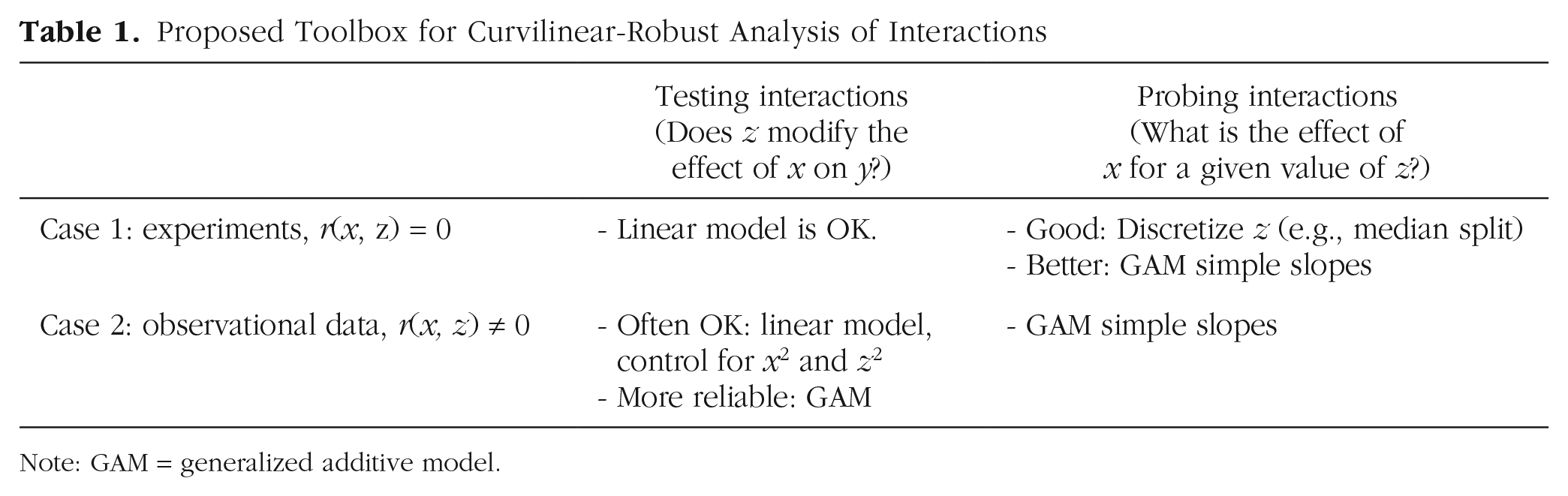
Note: GAM = generalized additive model.

In observational data, in contrast, one typically expects (most) variables to be correlated (Meehl, 1990), especially pairs of variables that are not chosen arbitrarily but, rather, are chosen because it is believed that both are associated with the same dependent variable. With observational data, then, one expects the omitted nonlinearities of x and z to correlate with x × z. In other words, when variables are measured rather than manipulated, incorrectly assuming linearity introduces bias in the interaction term (see e.g., Ganzach, 1997). ⁴

The preceding paragraphs involved Step 2, testing the interaction. When it comes to Step 3, to probing interactions, nonlinearities invalidate results both for data from experiments and from observational data. Figure 1 illustrates with the weight and gender example from before. Figure 1b highlights that there is a complex interaction between gender and age such that males get heavier than females starting at age 14 or so. A linear model cannot represent such a nonlinear interaction, and Figure 1c shows how when one relies on the linear model, one ends up projecting an incorrect sign reversal for babies such that baby girls are estimated to be heavier than baby boys.

Fig. 1.

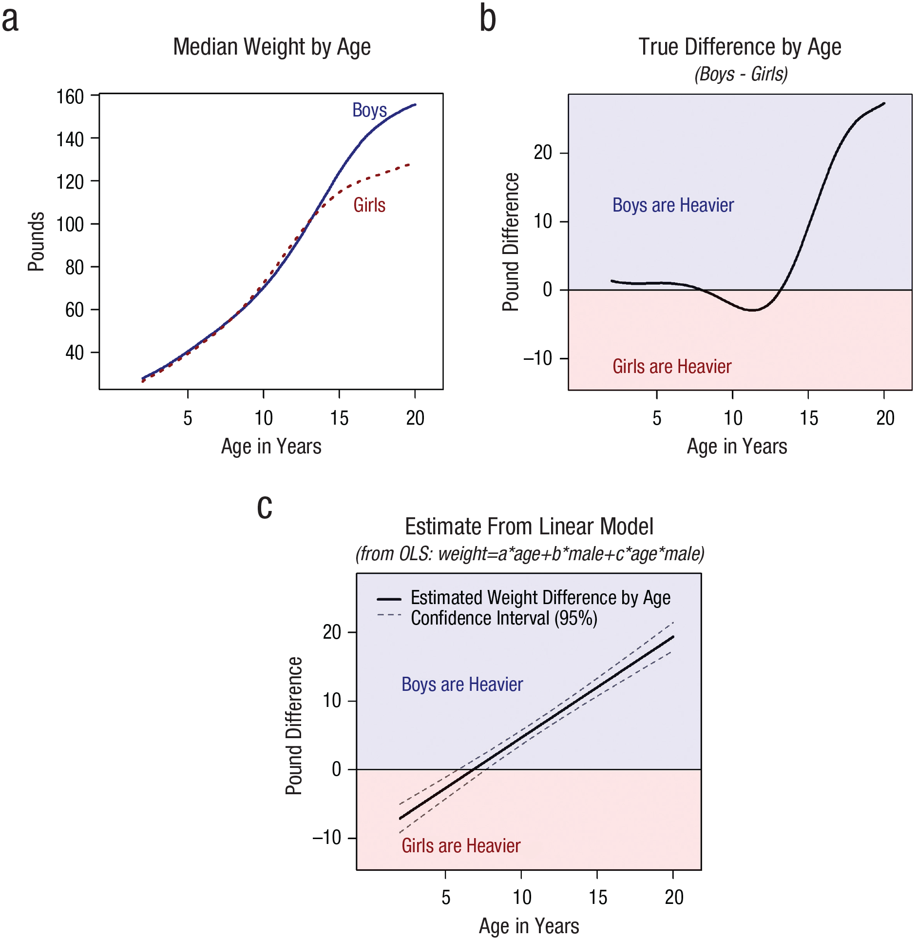
Nonlinear effects lead to misleading interaction results. R code to reproduce figure is available at https://researchbox.org/1569.2.

Figure 1c shows, then, that probing the interaction by plotting the effect of gender for all ages, that is, relying on the Johnson and Neyman (1936) procedure, one falsely but confidently concludes that baby girls are substantially heavier than baby boys.

In sum, nonlinearities invalidate the testing of interactions with observational data (in which x and z in x × z are expected to be correlated) and invalidate the probing of interactions in both experimental and observational data (i.e., even if x and z are expected to be uncorrelated).

There are good reasons to expect that nonlinearities, such as those depicted in Figure 1, are common in data collected by social scientists. From psychology, it is known that perception of change in physical and numerical stimuli exhibits diminishing rather than constant sensitivity (Fechner, 1860; Kahneman & Tversky, 1979). From economics, it is known that marginal benefit is diminishing rather than constant and that marginal cost is increasing rather than constant. In addition, many of the variables collected by social scientists consist of bounded scales that inevitably show diminishing rather than constant effects because some participants hit the ceiling or floor of the scale and can no longer be affected by further changes of the predictor of interest.

Any study that involves the perception of physical or numerical stimuli, the presence of costs or benefits, or measurement through scales, then, is likely to involve nonlinear relationships. Figure 2 provides some concrete examples of the kinds of nonlinear relationships observed in real data. A reviewer of this article remained skeptical of the proposition that one should generally expect nonlinear effects; readers sharing this skepticism can consult Supplement 6 in the Supplemental Material available online (http://researchbox.org/1569.82) and the excellent discussion by Ganzach (1997, pp. 244–245).

Fig. 2.

Examples of nonlinear associations in real data. In all figures, the lines are formed by fitting the data with flexible models (GAM for a and d; third-degree polynomials for b and c). (a) N = 47,729 survey responses from the General Social Survey (GSS). (b) N = 501 respondents to survey run by authors on attitudes toward genetically modified foods. (c) N = 956 survey respondents from the National Longitudinal Survey of Youth. (d) N = 12,427 interviews of applicants to an MBA program. This latter panel involves an article I coauthored with Francesca Gino, who was found guilty of academic misconduct after a near 2-year investigation by Harvard (for up-to-date information on this paper see https://manycoauthors.org/gino/95). R code to reproduce the figure is available at https://researchbox.org/1569.5.

Prior Work on Nonlinearities and Interactions

Just a handful of books and peer-reviewed tutorials appear to account for the vast majority of references social scientists use to guide the testing and probing of interactions (Aiken & West, 1991; Brambor et al., 2006; Cohen et al., 2003; Preacher et al., 2006; Spiller et al., 2013). Aiken and West (1991) alone accumulated, as of May 2023, more than 54,000 Google citations, and Preacher et al. (2006) accumulated another 5,500. These go-to references do not include discussions on how strong the linearity assumptions are (i.e., how at odds they are with what one should expect real-world data to look like) or how consequential the violation of such assumptions is. Possibly for this reason, few empirical articles have considered the impact of nonlinearities on the interpretability of the interactions they have reported. Although largely ignored by these tutorial pieces and most empirical work, some prior methodological articles have been concerned with the issues raised here.

Focusing on testing interactions, on establishing whether there is a statistically significant interaction, at least three articles (Cortina, 1993; Ganzach, 1997; Lubinski & Humphreys, 1990) have warned that if the effect of x or z on y are not linear and x is correlated with z, then the estimate of the interaction is biased, and its false-positive rate (FPR) is inflated. Throughout this article, I refer to this as the problem of “correlated nonlinear predictors.” The authors of these 1990s articles assumed that all nonlinearities are essentially quadratic and thus considered true models only of this form: y = a + bx + cz + dx × z + ex² + fz² + ε (see Note 5 for relevant quotes from these articles). ⁵

Upon assuming a true model that is quadratic, to address the problem of correlated nonlinear predictors, these articles naturally proposed researchers estimate quadratic regressions, that is, including x² and z² as covariates. In relation to this work, I relaxed the assumption that all nonlinear relationships are quadratic and relaxed the assumption that when x and z are correlated, their association is linear. Moreover, I empirically evaluated how well the proposal of including x² and z² as covariates performs for testing the x × z interaction with nonlinear correlated predictors and found it performs surprisingly well but not best; having higher FPRs and lower power than the generalized additive model (GAM)-based alternative proposed here.

In terms of probing interactions, on estimating the effect of x on y for different values of z, Hainmueller et al. (2019) discussed two problems with current practice (in political science). First, researchers sometimes probe interactions at moderator values for which no data exist, and second, sometimes interaction effects are nonlinear. ⁶ They introduced the “binning estimator” as an alternative to the linear probing of interaction to addresses these two shortcomings. The binning estimator splits the data into segments based on the moderator (e.g., low, medium, and high values of the moderator) and estimates separate linear models within segments. ⁷ The most important contrast between their work and the present article is that dichotomizing in general and the binning estimator in particular do not address the threat posed by correlated nonlinear predictors, a problem that was not mentioned by Hainmueller et al. Indeed, with observational data, the results obtained with the binning estimator are often as invalid as they are with the simple linear model it is designed to improve on (Simonsohn, 2023).

Finally, in terms of interpreting interactions, in terms of assessing whether a validly tested and probed interaction has the implications for the theory that motivated the study, Loftus (1978) made the important observation that when the variables one studies are proxies for the latent variables of interest, an observed interaction with measured variables need not imply an interaction among the latent variables (see also Krantz & Tversky, 1971). This observation is important and unfortunately has been largely ignored by researchers (Wagenmakers et al., 2012), but it is separate from the issues that concern this current article. Loftus’s observation is about the interpretation of statistically valid interactions, whereas this article is about the statistical (in)validity of interaction terms in linear models.

Alternatives to Assuming Linear Effects

I consider three main approaches for relaxing linearity assumptions: dichotomization, adding quadratic terms to a linear regression, and relying on GAMs. I provide overviews of the three approaches next and pay more attention to the more novel approach: GAMs.

Approach 1: dichotomization

The first and simplest approach for handling nonlinearities is to force linearity by dichotomizing the moderator. Rather than taking age as a continuous variable, one classifies boys and girls into, for example, above and below median age and carries out a simple 2 × 2 comparison of the four means. With dichotomization, the intuition goes, the linearity assumption (for the moderator) cannot be violated because two points always form a straight line. Dichotomization has long been relied on by social scientists, usually on grounds of its “analytical ease and communication clarity” (Iacobucci et al., 2015, p. 652). Dichotomization has also long been objected to by methodologists on grounds that it has lower statistical power (Cohen, 1983). ⁸ Considerations of lower statistical power aside, dichotomization has a subtler but more serious problem. As I demonstrate in a later section, when the two predictors in the interaction are correlated (e.g., what one generally expects when neither x nor z were randomly assigned), underlying nonlinearities in x can invalidate interactions with median splits of z as much as they invalidate interactions with continuous z. Thus, for testing interactions between correlated nonlinear factors, median splits suffer from elevated Type 2 and Type 1 errors.

Approach 2: adding quadratic controls (x² and z²)

As mentioned above, a few authors have advocated for including quadratic terms of x and z when estimating regressions with the purpose of testing an x × z interaction (Cortina, 1993; Ganzach, 1997; Lubinski & Humphreys, 1990). They conjectured that quadratic controls were sufficient to deal with any nonlinearity (see Note 5 here), but they did not evaluate such conjecture. They did not carry out simulations assessing how well quadratic controls work if real functional forms are neither exactly linear nor exactly quadratic. I carried out that evaluation here. As I show later, I found that quadratic controls perform surprisingly well under a broad range of (nonquadratic) functional forms but that they are on occasion insufficiently flexible to ensure valid inferences in the presence of realistic nonlinearities. Quadratic controls, moreover, can lead to substantially lower statistical power than do the procedures proposed in this article. Finally, when it comes to probing interactions, to assessing how big the effect of x on y is for different values of z, quadratic controls lead to correct estimates only if the true functional form is quadratic, an arbitrary and (practically speaking) untestable assumption.

Approach 3: GAMs

A third approach moves one away from arbitrary assumptions about functional from (quadratic) and arbitrary dichotomizations (median split) and toward estimating the functional form of interest. A few procedures allow flexible functional form estimation (e.g., locally estimated scatterplot smoothing, kernel regression), but the one that seems most applicable to a broad range of data structures, in terms both of analytical flexibility and computational efficiency, while providing interpretable enough estimates is GAMs (Hastie & Tibshirani, 1987; Wood, 2017).

Although GAMs were developed decades ago, they have not been used much in psychological research yet. ⁹ I hope this article will change that. GAM is conceptually similar to linear regression in that they both estimate the relationship between predictor variables and a dependent variable. The key difference is that regressions assume all entered effects are linearly associated with the (sometimes latent) dependent variable, whereas GAMs estimate the functional forms of each effect. ¹⁰

From a user perspective, relying on GAMs can be quite similar to relying on linear regressions. I next illustrate with a simple example, written in R, in which data are analyzed with a linear regression and with a GAM side by side. I start simulating data, making variables x, z, and e be (standard) normal and making y depend linearly on them:

One can estimate a linear regression with:

And one can estimate a GAM with:

In the GAM, s() indicates a “smooth” (flexible functional form) main effect, and ti() indicates a flexible interaction term. The output for lm1 is one researchers are familiar with: four point estimates. The GAM, like the linear model, produces four p values: for the intercept, the two predictors, and their interaction. But when it comes to the coefficient estimate, interpretation is more difficult. For the example above, for instance, GAM produces 35 instead of four coefficients. I argue here one should tolerate GAMs’ harder to interpret output for two key reasons. First, GAMs’ output is more likely to be statistically valid and descriptively accurate. As I show later in this article, the linear model’s easy to interpret results can be extremely misleading and statistically invalid, especially for interactions. One can more easily read the output from a regression, then, but that easy to read output from the regression is also too easily wrong. The second reason I think one should tolerate GAMs’ harder to interpret output is that one can make it interpretable without much effort, relying on the same techniques researchers rely on to make regression coefficient estimates for interactions interpretable, the aforementioned simple slopes (Aiken & West, 1991).

As interpretable as the output for a linear regression seems, when interactions are involved, it is actually not that easy to interpret. As researchers, we want to know “the” effect of x on y, but when an interaction is involved, there may be infinite effects of x on y, one for each possible value of z. This is why to interpret regressions, researchers probe them (Aiken & West, 1991). With simple slopes in particular, researchers compute the expected value of y for all values of one predictor, keeping the other predictor(s) fixed at a given value.

Returning to the simple example above, the estimated regression equation is y = .02 + 1.06x + 1.06z + .975x × z. If one is interested in “the” effect of x on y, that regression equation gives a different estimate for every possible value of z. With simple slopes, one would fix z at some point, for example, z = 1, and plot the relationship between y and x for z = 1. With GAMs, researchers can do the same calculation, reducing the interpretability disadvantage that GAMs suffer from. Moreover, simple slopes for the linear model and for GAM can be estimated with the same (wrapper) function in R, “predict.” ¹¹ The code below carries out simple-slope calculations for the linear model and for GAM:

The first line of code generates the values of x that are of interest for probing, going from −2 to 2 in increments of .1. The second line of code produces the expected value of y, given the linear model results, for x values between −2 and 2 when z = 1. The third line does the same given the GAM results.

An (older) alternative to simple slopes is the Johnson and Neyman (1936) procedure (also known as “floodlight analysis” and “regions of significance”). It estimates the marginal effect of one variable for every possible value of the other. In this article, I focus on and advocate for GAM simple slopes rather than GAM Johnson Neyman because depicting the levels of the dependent variable, rather than the marginal effects, makes it easy to give results a proper contextualized interpretation. But GAM Johnson Neyman is easy to implement as well. For an example with R code, see Supplement 5 in the Supplemental Material (https://researchbox.org/1569.82).

GAMs can be applied to a wide range of data structures. One can estimate a GAM when the dependent variable is binary or categorical (in lieu of probit or logit regressions). One can also include random effects into GAMs (Simpson, 2021; Wood, 2013, 2017) and estimate multilevel models (see e.g., the gamm4 package in R).

GAMs’ estimation procedure includes a penalty for overfitting; in practice, this means that if an association is best described by a linear model, GAMs will tend to deliver a linear model, but if it is best represented by a cubic function, sine function, or combination of the two, it will tend to deliver that instead. The performance of GAMs in recovering functional form is impressive for researchers who still rely on the 19th-century technology of fitting data with straight lines. See Figure 3.

Fig. 3.

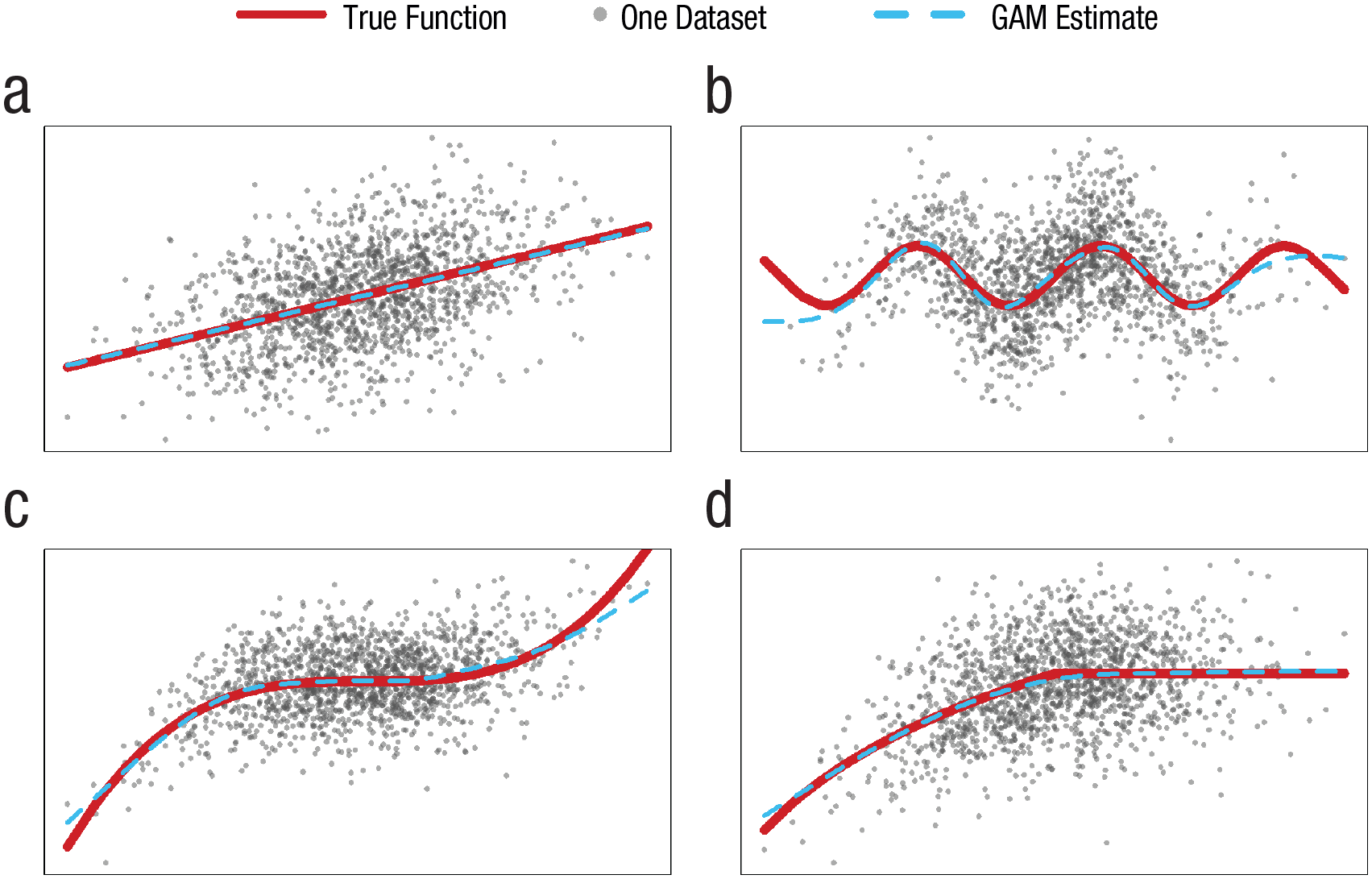
Examples of GAM correctly recovering underlying functional forms. The four figures are based on the same draw of N = 1,500 x values dawn from N(0, 3), with the y values corresponding to (a) y = x, (b) y = sin(x), (c) y = x³ – x², and (d) min(log(x + 14),log(14)). Random noise N(0, SD) was added, with SD equal to twice the standard deviation of Y caused by x. R code is available at https://researchbox.org/1569.15.

In the next section, I demonstrate the application of GAM simple slopes to data from psychology articles, but first, in a short subsection, I provide a quick summary of the proposed toolbox I put forward in this article for testing and probing interactions in social science.

Toolbox preview

The goal of this article is to deliver a curvilinear-robust toolbox for studying interactions in social science. In the remaining sections, I motivate and demonstrate the tools in the proposed toolbox by reanalyzing published data. I then evaluate the validity of the tools, for a broad range of scenarios, via simulations. Anticipating the conclusions of these analyses, I provide a summary of the proposed toolbox in Table 1.

Examples of GAM Simple Slopes With Data From Psychology Articles

In this section, I report simple slopes, both linear and GAM, constructed using data from two published articles. I first return to the MBA interview data from Figure 2d. The data set includes applicants’ work experience and country of origin. A linear regression using these variables to predict interview score results in: score = 2.2 + .013 × Experience – .166 × American + .005 × American × Experience.

Figure 4 shows the linear simple slopes implied by that equation. We learn that Americans benefit more from experience and that the gap grows, linearly of course, with experience. The narrow confidence bands imply statistically significant differences for almost every level of experience. ¹²

Fig. 4.

Linear versus GAM simple slopes reanalyzing data from Simonsohn and Gino (2013). N = 11,740 interviews of applicants to an MBA program. Applicants were rated on a scale from 1 to 5. The figure reports results of predicted scores for the interview based on models with two independent variables: work experience of applicant (M = 44.9 months) and whether they are American (M = 61%). Because of outliers in terms of experience, corresponding to possible coding errors, data were truncated at 200 months of experience. GAMs were estimated separately for American and non-American applicants: gam(y ~ s(x,k = 5)). A Johnson-Neyman version of this figure and robustness simple-slopes plots with different cutoffs and k values are presented in, respectively, Supplements 1 and 2 in the Supplemental Material available online. R code to reproduce figure is available at https://researchbox.org/1569.18.

To accompany the visual display of simple slopes, I report also statistical contrasts comparing the predicted y value of the two plotted curves for a few values in the x-axis. I use as defaults the median and the 15th and 85th percentiles; the latter two correspond roughly to the mean ±1 SD for a normally distributed variable. One can think of those three contrasts as points in the Johnson and Neyman (1936) curve. ¹³ For instance, the first such contrast in Figure 4a indicates that the estimated effect of being an American applicant, among participants with very little experience, is negative and highly significant in the linear model and much smaller and with a higher p-value in the GAM.

Although the three contrasts are of the same sign across the linear model and GAM, quantitatively, the linear model’s contrast are substantially larger (between 50% and 100% larger). Much more interesting in this case, however, is the qualitative comparison of the overall shape of the simple slopes.

Note that the GAM suggests that (a) scores do not continue to diverge by more and more with greater experience, (b) the two lines are essentially identical up to 3 years of experience, and (c) overall, the benefit of experience plateaus rather than continues to increase at a constant rate throughout. The picture that arises from the GAM simple slope is richer, and it is based on the data rather than on arbitrary assumption about the data. If one assumes the impact of experience on interview scores is linear, the model will show that the effect of experience on interview score is linear, but one is not really learning from the data (in this regard); one is, instead, imposing on the data.

Figure 5 provides a second example, this one based on data collected by Lawson and Kakkar (2022). Their core hypothesis was that “the sharing of fake news is largely driven by low conscientiousness conservatives [italics added]” (p. 1154). Note that here, the dependent variable is binary, and thus the “linear” simple slopes is linear in the “generalized linear models” sense, in which a logit regression is considered a linear model.

Fig. 5.

A hypothesis receiving stronger support with GAM simple slopes. (a) Reproduction of the probed interaction reported by Lawson and Kakkar (2022; see their Figure 5, but see Note 12 here). It was generated by estimating a logistic regression on 967 participants, with 24 observations each (N = 23,208) and then plotting predicted probabilities to share news; simple were slopes computed at 2.5 and 4 of conscientiousness (for justification, see Note 20). (b) Equivalent calculations relying on a GAM (gam(y~s(x,k = 4), method = “REML,” family = “binomial”). Contrasts comparing the two simple slopes are reported at 1, 4, and 7 in the political orientation scale (there are 127, 176, and 74 respondents at each of those three buckets, respectively). The confidence bands were computed via bootstrapping, by randomly resampling participants, rather than rows, to maintain the dependence across observations in the resamples. For an alternative approach, see Note 21. The confidence bands depict the values obtained in the 95% less extreme resamples. R code to reproduce the figure is available at https://researchbox.org/1569.35.

The GAM simple slopes allow for a more focused and supportive, in this case, evaluation of the prediction that the effect of interest is driven by conservatives. Looking again first at the contrast at the 15th quantile of the focal predictor, one sees that although the linear model indicates a reversal for very liberal participants, the GAM suggests such reversal may be spurious, arising from imposing linearity on all effects (like the heavier baby girls in Fig. 1).

Lin et al. (2023) noted that Lawson and Kakkar’s (2022) result should not be interpreted as supporting an effect on the sharing of fake news because low-conscientiousness conservatives were more prone to sharing in general, not only fake news. They also reported five conceptual replications of the studies by Lawson and Kakkar that did not replicate the interaction. I have chosen to keep this example here despite its apparent lack of robustness because only upon producing GAM simple slopes on the data collected by Lin et al. did I become convinced of their failure to replicate. It does, therefore, illustrate the practical use of GAM simple slopes: providing more informative descriptions of interaction results. Not being an expert, I do not take a position on the substance of this debate on the sharing of fake news.

Having illustrated the similarities and differences between linear and GAM simple slopes, in the next subsection, I rely on simulations to contrast their performance for probing interactions when at least one of the two variables in the interactions was randomly assigned (i.e., in experiments).

Probing Interactions in Experiments (When at Least One Factor in x × z Is Randomly Assigned)

FPRs for probed interactions

In this section, I rely on simulations to evaluate the performance of three alternative tools that can be used to probe interactions: (a) dichotomization (median split), (b) linear simple slopes, and (c) GAM simple slopes.

For the simulations in this section, I considered experiments in which treatment x is randomly assigned (x = 1 or x = 0) and the true association between x, z, and y involves an attenuating interaction: The effect of x on the dependent variable, y, is reduced but never reversed by a moderator variable, z. For example, the true model y = x/z, with z > 0, meets this description; bigger z values reduce the effect of x but never reverse it. Focusing on attenuating interactions simplifies the reporting of results: I report how often each tool used to probe interactions falsely concludes the effect of x on y flips in sign with high enough zs when in fact it never does.

In terms of the true associations, as is detailed in the caption for Figure 6, I considered two baseline scenarios: a linear effect with a ceiling and concave smooth function. For each, I created 36 variations with different sample sizes, functional forms, and distributions of the moderator variable. Each of the resulting 72 variations were used to run 5,000 simulations, which kept track of how often a false-positive sign reversal was detected.

Fig. 6.

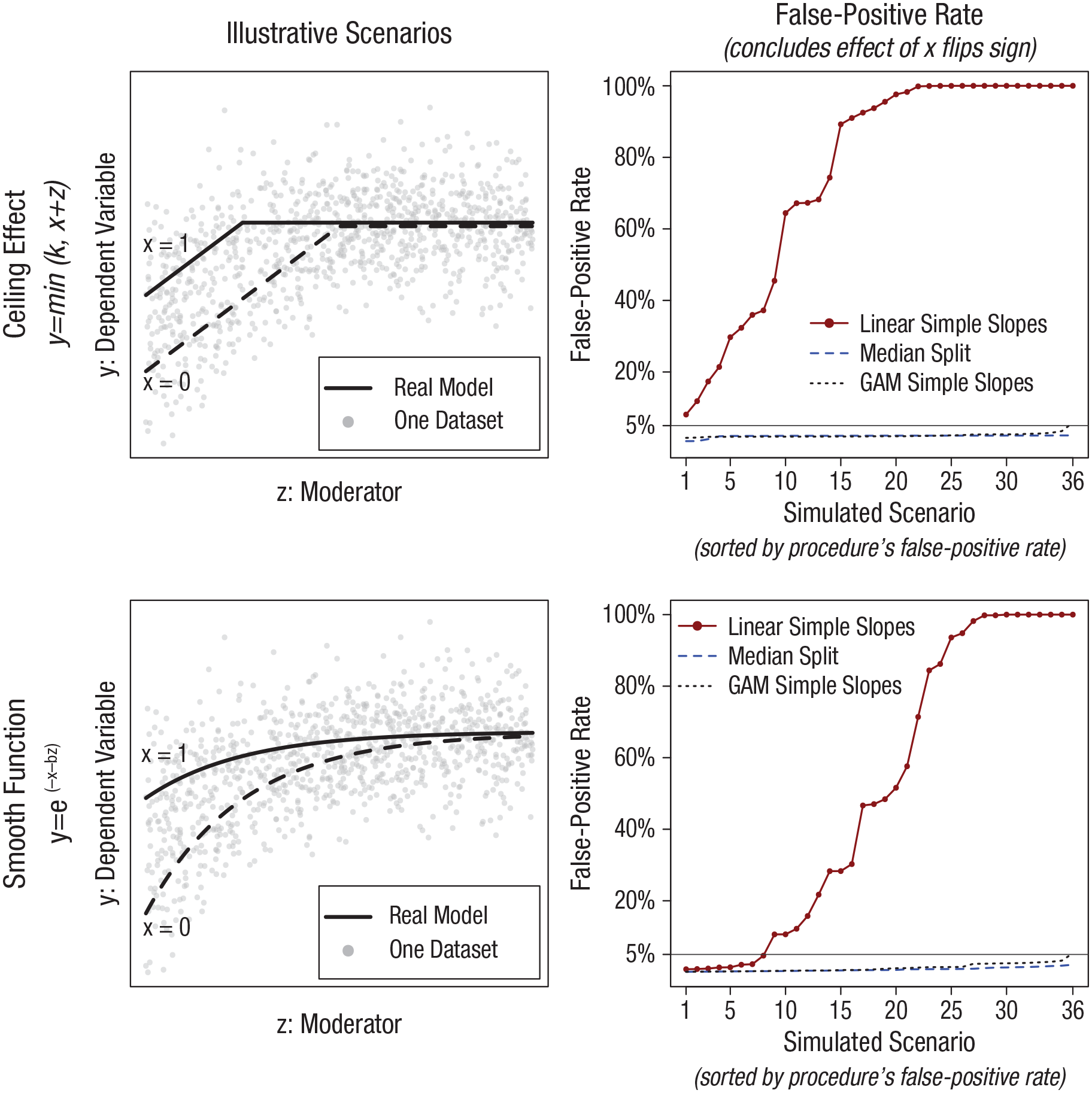
False-positive rates for effect of x on y being negative for high z; true effect is never negative. The y-axes depict the percentage of 5,000 simulations, run for each of 72 scenarios, in which the probing of an interaction between x and z lead to an estimated negative effect of x on y, with p < .05, for a high z value despite the true effect never being negative. In all simulations, x is binary, and scenarios are generated by varying the distribution of z (standard normal, left-skewed, right-skewed, uniform; the latter three range between z > –2 and z < 2) and sample size per condition ns = 100, 200, or 500. Figures in the left show scenarios that vary the ceiling for the effect of x and z on y to –.5, 0, or +.5 (a ceiling effect before adding random noise). Figures in the right show scenarios that vary the coefficient of b to be 1, 2, 3. These operationalizations lead to the 4 × 3 × 3 = 36 scenarios in each figure. The plotted false-positive rates are adjusted by expected simulation error (deviation from a true rate of 5%) for 1st, 2nd, . . . 36th most extreme post hoc value of simulation error. R code to reproduce the figure is available at https://researchbox.org/1569.80.

For linear and GAM simple slopes, I consider a result to be false-positive when the effect of x is estimated as significantly negative, p < .05, when the moderator is at 85th percentile of its observed values (again, the true effect of x is never negative no matter what value z takes). For the median split, I consider a result to be false-positive when the slope for the above-median moderator values is negative and p < .05.

Valid statistical tests have a FPR, for p ≤ .05, no greater than the nominal 5%. The poor performance of linear simple slopes depicted in Figure 6 is striking. For many scenarios, the approach that is the current “gold standard” for much of social science for probing interactions achieves a 100% FPR; it always arrives at statistically significant evidence of something that does not, in fact, exist. The two alternative approaches, in contrast, are slightly conservative for most scenarios and close to the 5% nominal rate even in the most extreme ones. ¹⁴

Going beyond p values and FPRs for comparing statistical approaches, I note that if a procedure has an inflated FPR, then one knows its confidence interval will not have proper coverage; thus, deciding which model to estimate based on confidence interval performance, rather than FPR, would also discourage relying on linear simple slopes. In terms of model fit, the mean squared error for the linear model is, across the 72 scenarios, between 3 times and 13 times larger than for GAM. Because these are simulated data, one can compare fit in terms of the ground truth. That is, instead of asking how well a model fits the (simulated) data, one can ask how close to the truth is each estimated model. In addition to its intuitive appeal, this approach to assessing model fit builds in protection against overfitting. GAMs could have lower MSE by overfitting the data, but they cannot get closer to ground truth by overfitting the data. If a model is reading random error as signal, then it is going to get further from the ground truth. I thus also computed a “truth-MSE,” the average squared error between each observation’s true y value and the fitted value based on the models. It is not close. Across the 72 scenarios, “true-MSE” is between 10 times and 382 times higher with the linear model.

Why do GAM simple slopes outperform?

To illustrate why GAM simple slopes outperform linear simple slopes, Figure 7 depicts results for one of 5,000 simulations for one of the 72 scenarios depicted in Figure 6. It illustrates how the arbitrary linearity assumption forces a spurious sign reversal for the estimated effect of x on y. This is again analogous to the heavier baby girls from Figure 1 and the apparently spurious reversal of the impact of conscientiousness for very liberal respondents in Figure 5.

Fig. 7.

Example of simulated scenario in Figure 6 with high false-positive rate for linear model. The three figures depict the same simulated 500 observations per condition (x = 1 vs. x = 0). The true functional form is y = 1 − e^-(x+b×z). R code to reproduce the figure is available at https://researchbox.org/1569.26.

Statistical power for probing interactions in experiments

Here, I consider the power properties of GAM simple slopes for experimental data (in which either x or z in x × z was randomly assigned). The FPRs of the linear simple slopes shown in the previous subsection seem sufficiently high to justify abandoning the approach even if it provided higher statistical power than the alternatives. But note that linear simple slopes can easily have lower statistical power than even the median split. To appreciate this, one does not need new simulations. Look back at the right figure of Figure 6. For high values of z, simple slopes estimate the effect of x as negative, in the most extreme cases with FPRs of 100%; thus, the model has a 0% chance of detecting the actual positive effect.

In other words, although median splits have been justifiably criticized for decades for having lower power than the linear model to test interactions (Cohen, 1983), they can have greater power for probing those interactions. Just to be safe, I state this again. The long-standing claim that dichotomization lowers power for testing an interaction is correct. What does not follow from this true fact, however, is that a linear simple slope is a more powerful approach for probing an interaction. By avoiding specification error, the median split can outperform linear models when probing interactions (again, in experiments, when one factor in x × z is randomly assigned). Nevertheless, it is generally the case that the median split will have lower power for probing interactions than will GAM simple slopes. Unless one is unable to implement a GAM simple slope, then, a median split is not the best option for probing interactions.

It is interesting to consider, as a boundary case, the unlikely scenario in which the true model is perfectly linear. How much less power do GAM simple slopes have to probe such interactions in experiments compared with linear simple slopes? Figure 8 reports encouraging results. Across 16 scenarios, varying the distribution of the moderator and the slopes involved in the linear interaction, GAM simple slopes achieve a very similar level of precision/power as do the linear simple slopes. The intuition is that GAMs build in protection against overfitting, and thus, they report linear effects when true effects are linear. After paying a small penalty in power for the functional-form flexibility, one gets linear-model estimates with GAM when the true model is linear. ¹⁵

Fig. 8.

Relative power for linear versus GAM simple slopes. The bar plots depict the statistical power, obtained by GAM simple slopes, testing the null that the effect of x is zero when the moderator z is at its 85th percentile. The simulated functional form is perfectly linear and calibrated across scenarios to have 50% or 80% power for linear simple slopes. Across the 16 scenarios, the simulations vary the distribution of the moderator z (to be uniform, beta, or normal), the size of the interaction (true coefficient for x × z), and the sample size. R code to reproduce the figure is available at https://researchbox.org/1569.30.

In sum, switching from linear to GAM simple slopes to evaluate experimental results would (a) eliminate the threat of possibly high FPRs when effects are not linear, (b) substantially increase power in some cases when the true effect is not linear, (c) improve the qualitative overall characterization of the relationship of interest, and (d) not meaningfully reduce power in the unlikely scenario of an actual linear relationship. There do not seem to be any reasons to continue relying on linear rather than GAM simple slopes.

Testing Interactions With Observational Data (With Measured Rather Than Manipulated Variables)

In the previous section, I covered the probing of interactions composed of predictors expected to be uncorrelated (e.g., where x or z in x × z was randomly assigned in an experiment). In this section, I move on to (a) testing rather than probing and (b) interactions in which x and z could be correlated (e.g., when both x and z are measured rather than manipulated).

As explained in the introduction, the challenge curvilinear relationships pose to testing interactions is a special case of the challenge omitted variables pose to testing regression coefficients more generally. When one omits a relevant variable from a regression, coefficients for included variables that correlate with the omitted variable can be biased, and thus omitting the nonlinear portions of x and z bias the estimate of x × z. This is why incorrectly assuming linearity when testing the x × z interactions is OK in experiments in which x or z was randomly assigned (because x × z will not correlate with omitted nonlinear terms), but it is not OK when x and z could be expected to be correlated because the omitted nonlinear portions of x and z are expected to correlate with x × z and thus bias its estimate.

Example of an invalid interaction test in data from a published article

Preacher et al. (2006) probably constitutes the most cited peer-reviewed article giving researchers guidance on how to probe regression interactions. I reanalyze here the only example in that article (see their section, “An Example,” pp. 444–446). The data set, from the National Longitudinal Survey of Youth, involves 956 children as the unit of analysis; performance on a math test as the dependent variable, y; and measures of children’s antisocial tendencies, x, and hyperactivity, z, as the key predictors. Preacher et al. used this data set to illustrate the use of (linear) simple slopes. Here, in contrast, I am not interested in probing the interaction but in testing it. Despite being a tutorial on the interpretation of interactions, Preacher et al. did not discuss the issue of interest here, the invalidating impact of correlated nonlinear predictors.

Estimating the linear model in their article, I perfectly reproduced the reported point estimate and p value for the focal interaction (b = −0.3977, p = .0055). ¹⁶ Figure 9, however, shows that for this data set, one should expect and actually observes the linear model having an inflated FPR for the interaction.

Fig. 9.

Correlated nonlinear predictors in Preacher et al. (2006) invalidate their interaction results. (a, b) Mean values of the dependent variable for each possible value of the predictors. (c) Scatterplot and best fitting regression line for the predictors. (d) False-positive rates for testing the x × z interaction for four alternative models. R code to reproduce the figure is available at https://researchbox.org/1569.33M.

Figure 9a shows that at least one predictor in the interaction has a likely nonlinear effect, and Figure 9c shows that both predictors are correlated. As explained earlier, correlated nonlinear predictors bias the interaction term, which will typically raise the FPR. Figure 9d reports that the estimated FPRs are indeed well above the nominal 5%. I computed FPRs by simulating data under the null, forcing the absence of an interaction, and assessing how often the linear model obtained a statistically significant interaction. For details, see Supplement 3 in the Supplemental Material.

Preacher et al. (2006) used these data to demonstrate the calculations and interpretations of probed interaction; it is likely that the ultimate correctness of the model they estimated was of secondary importance to them. ¹⁷ Thus, my analyses are not meant as a narrow criticism of how they analyzed this data set but as a general point about how we as a discipline have long overlooked the invalidity of linear models to study interactions. Even researchers writing tutorials about interactions have overlooked it.

Having provided the intuition for the problem correlated nonlinear predictors pose for testing x × z interactions, in the next subsection, I explore the performance of alternative tools for testing interactions in the presence of correlated nonlinear predictors.

Simulations and the FPRs testing interactions between correlated nonlinear predictors

The goal of the simulations reported in this subsection is to assess the performance of the alternative tools for testing interactions in a very broad range of scenarios involving nonlinear effects. The alternative tools considered, which I contrast to the traditional approach of testing the coefficient of x × z in the linear regression model, involve (a) dichotomizing the moderator, (b) adding quadratic x² and z² as covariates, and (c) estimating a GAM instead of a linear model. Because I found that the GAM p values are incorrect (I relied on the R package mgcv that comes bundled with R), I also report results for GAMs with bootstrapped p values.^18,19 As a preview of the results, this latter approach, “bootstrapped GAM,” is the only one that performs adequately in all scenarios considered.

To avoid stumbling on a simulated scenario that by chance happens to make one tool work better than the other, I created 3,840 scenarios through the exhaustive combination of several of the key operationalizations behind the simulated data. Figure 10 shows stylized depictions of those operationalizations.

Fig. 10.

Operationalizations for computing false-positive rate of interaction with correlated predictors. R code to reproduce the figure is available at https://researchbox.org/1569.37.

For example, one of the 3,840 scenarios involved x having a skewed-high distribution, while being correlated r = .5 with z through a log-linear relationship, in which x has a cubic effect on y and z has a log-canopy effect on y, studied with 750 observation. In consideration of computing time, I randomly selected 300 of these 3,840 scenarios and simulated 5,000 data sets for each scenario. For each, I tested for an interaction using the five aforementioned analytical tools. Because there is no interaction in any of the scenarios, all obtained p < .05 results are false-positive. A curvilinear robust tool for testing interactions should thus obtain p < .05 in about 5% simulations for each of the 300 scenarios considered. The actual proportions of p < .05 for each tool are depicted in Figure 11.

Fig. 11.

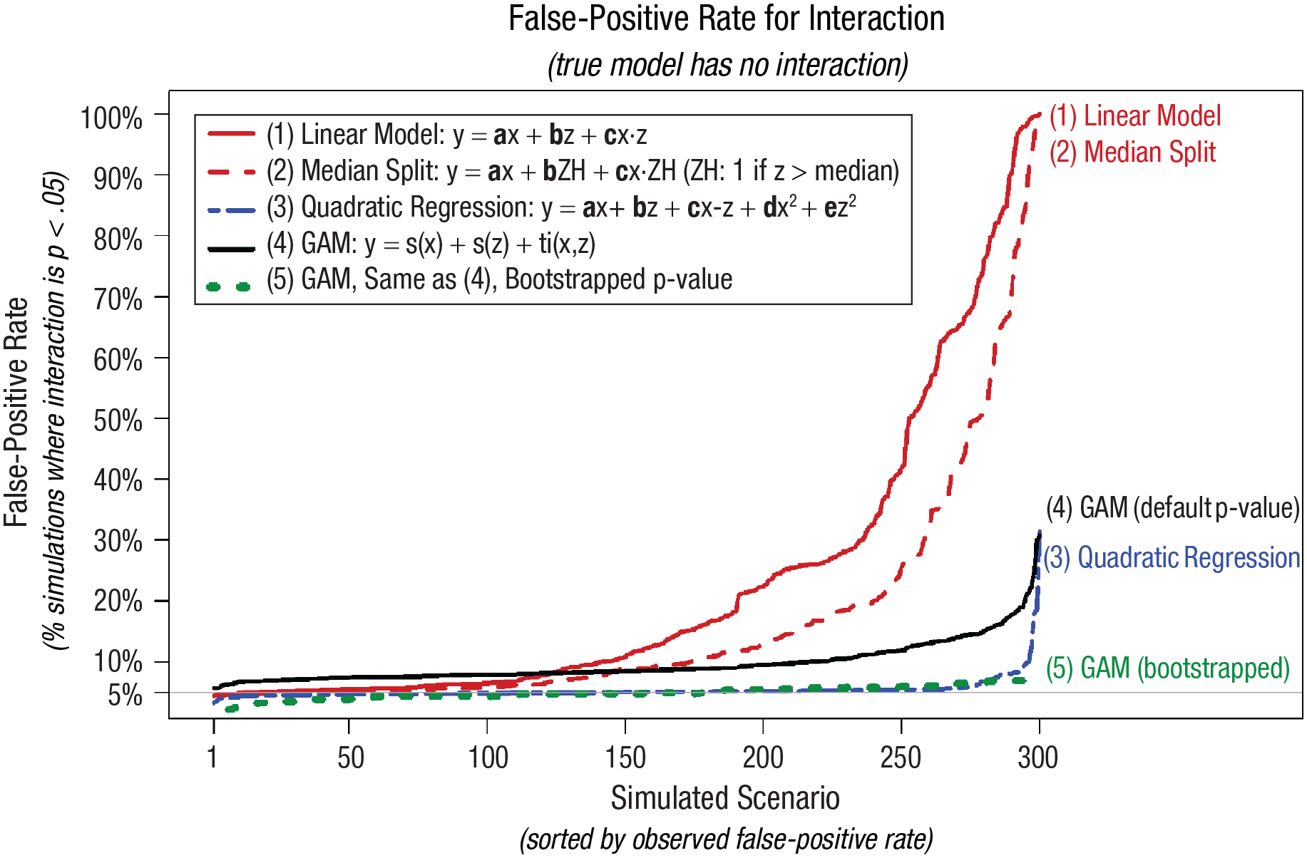
False-positive rates (FPRs) for interactions with nonlinear and correlated x and z predictors. The y-axes depict the percentage, out of 5,000 simulations, for each scenario in which the interaction term obtained a statistically significant result (p ≤ .05) despite the true interaction being zero. The 300 simulated scenarios are generated combining the operationalizations depicted in Figure 10 (a random subset of 300 out 3,840 scenarios were run). The GAM was estimated using R’s “recommended” package, mgcv, with syntax: gam(y~s(x)+s(z)+ti(x,z)). The bootstrapped GAM p value for the interaction smooth is obtained by first estimating a model without the interaction, gam(y~s(x)+s(z)), and then using this “null” model to generate 100 (wild) bootstrapped samples, adding to each predicted value the observed residuals from that model, each multiplied with independently drawn at random 1 or −1. This is repeated 100 times, and the adjusted p value is the share of these bootstrapped samples in which the p value for the interaction, in gam(y~s(x)+s(z)+ti(x,z)), is at least as low as that obtained in the observed data. Given computational costs, a sample of the 300 scenarios were reran with bootstrapping. Specifically, I reran the 20 scenarios with the highest FPR for the GAM model and then every 10th scenario below the 280th (so, the 270th highest FPR for the GAM interaction, the 250th highest, etc.). For more details, see Supplement 4 in the Supplemental Material available online. R code to reproduce the figure is available at https://researchbox.org/1569.42.

First, I show that the linear model and the median split are strikingly invalid for the majority of scenarios considered. It is worth emphasizing that approximately all articles in social science that test interactions rely on one of these two tools. This does not mean, however, that all published interactions are false-positive. In fact, almost surely many are not.

Second, and surprisingly, the simple solution of merely adding x² and z² to the linear model (Cortina, 1993; Ganzach, 1997; Lubinski & Humphreys, 1990) achieves near nominal FPRs in the vast majority of scenarios considered despite the presence of specification error (in none of the models is any true relationship exactly quadratic). It is worth pointing out that although adding quadratic controls has been advocated for in several articles, this seems to be the first effort to systematically evaluate how such solution performs when the assumed functional form, quadratic effects of x and z, is not correct. Although the idea of using quadratic controls is old, evidence that this is a good idea is new.

There are a few specifications, however, in which this approach suffers from markedly inflated FPRs, falsely rejecting the null more than 25% of the time. It is ultimately an empirical and difficult to answer question whether functional forms in the real data sets analyzed by social scientists tend to look like the majority of scenarios in which the quadratic controls fix the problem at hand or like the minority of scenarios in which it does not. For what it is worth, returning to the Preacher et al. (2006) example discussed in the previous section, adding quadratic controls leads to the nominal 5% FPR for the linear model. Returning to the simulation results from Figure 12, I show that although the p value from the GAM overrejects the null, the bootstrapped p value performs well for all scenarios considered, although it does go over 1 to 2 percentage points above 5% for some scenarios.

Fig. 12.

Statistical power to detect an interaction when true functional form is and is not linear. Each row reports estimated power for one scenario, depicted in the first column, varying the correlation between the factors in x × z. Every simulation has 500 observations, and x and z are normally distributed. Negative power indicates the probability of obtaining a p < .05 result for the interaction with the wrong sign.

Note that in the absence of the bootstrapping correction, the quadratic solution outperforms GAMs. I return to the relevance of this poor performance of p values generated by the GAM procedure in the general discussion

Simulations and statistical power for testing interactions with correlated predictors

In the previous subsection, I demonstrated the superior performance of GAMs over linear models, in terms of false-positive rates, when the true functional form is not linear. A relevant question is the price paid in terms of power to achieve this lower Type 1 error rate. As before, I consider the corner case when the true model is linear, but I also consider the case when the true model is not. See Figure 12.

I show that when x and z in x × z are uncorrelated, there is essentially no difference in power across the four procedures. The more correlated x and z are, the higher the consequences of misspecification are (as mentioned before, this is because the omitted nonlinear portion of an effect is then correlated with the interaction and thus biases it). Overall, although there are scenarios for which switching to GAMs imposes power losses, these tend to be small losses. In addition, in more realistic scenarios, in which functional form is not perfectly linear, GAMs offer higher power than the current tools in the social-scientist toolbox do, possibly much higher power. Note that in some of the scenarios in these figures, the linear model has very high “negative” power, a high probability of obtaining p < .05 for an effect of the wrong sign. It is difficult and perhaps impossible to be confident about functional form in social science, and when functional form is uncertain, GAMs offer better expected performance in terms of both Type 1 and Type 2 errors.

GAMs’ Limitations

Having advocated for GAMs through most of this article, in this section, I discuss what I consider to be its four main limitations.

Limitation 1: interpretability

A commonly raised shortcoming for GAMs is that their black-box nature makes them “somewhat less interpretable than linear regression” (G. James et al., 2021, p. 309). This shortcoming, however, is not too difficult to circumvent by expressing GAM results in familiar forms, such as GAM simple slopes. Interactions even in linear models are actually difficult to interpret, which is precisely why researchers probe them, computing linear simple slopes. As I have shown throughout the article, GAM simple slopes are easy to produce and just as easy to interpret as linear ones.

In addition, it seems odd to give any weight to interpretation ease when the alternative, the easier to interpret result, is simply wrong. Imagine a choice between two watches: a digital watch with large and easy to read numerals but broken, permanently stuck at an easy to read “3:45:00 PM” versus an analog watch without any numerals but always showing the correct time of day. One would not give any weight to interpretation ease when choosing between these watches.

Limitation 2: specification ambiguity

Linear regressions have relatively few options in terms of implementation, concerning primarily how standard errors are computed (e.g., relying on robust, clustered, or homoskedasticity-assuming standard errors). GAMs, in contrast, have many options, from the estimation procedure (e.g., REML vs. GCV) to the penalty for overfitting to whether the number of knots is preset or estimated to the flexibility (number of base functions) behind any particular smooth. Software that implements GAMs does make default choices for all of these, but those defaults may change over time and differ across statistical packages. Moreover, any user can opt out from these defaults when analyzing any given data set. This specification ambiguity poses two main challenges, one for authors and one for readers.

In terms of authors, they must somehow make all those decisions, and they may not have a priori basis or sufficient understanding to do so (in fact, probably most GAM users lack both, especially if GAMs become popular as quickly as I hope). In terms of readers, simply reading from an article that a GAM is behind a particular result is not enough to know just what the authors did. This challenge of specification ambiguity, which affects authors and readers, does seem important but is manageable.

First, default values do tend to be sensible and are not often consequential; absent additional information, using the default is a good strategy for most situations. For example, a reviewer asked that I change the estimation procedure for all calculations in this article, from the current default in the R package, GCV, to an alternative that may become the default in the future, REML. I did, and not a single figure or result was perceivably affected by this choice. Second, for transparency’s sake, when a researcher deviates from default settings, it seems advisable to report results for a few alternative settings, ensuring results do not hinge on a specific and possibly arbitrary choice or that if they do hinge, that this fact is shared with readers (e.g., “We find an interaction but only when using REML, not GCV, this may be because . . . ”). Third, in terms of reproducibility, articles that rely on GAM estimation should include in the main text the exact specification ran, for example, a footnote that reads “Using the mgcv package Version 1.8-41, we estimated the model gam(y~s(x)+(z)+ti(x,z)).”

Before moving to the next limitation, I note that specification ambiguity is not unique to GAMs. Although linear regressions do not have much ambiguity, many other methods already popular in social science do, including “mixed models,” structural equation modeling, factor analysis, meta-analyses, and so on. Specification ambiguity is a good reason to show robustness or explicitly justify choices; it is not a good reason to avoid a tool altogether. It would be desirable for articles that rely on those methods to also report the exact specification run so that readers can find out, for example, whether a mixed model included only random intercepts or also random slopes.

Limitation 3: wrong p values

The third GAM limitation I consider is that its p values are often simply wrong, exhibiting much larger than nominal FPRs (see e.g., Fig. 11). This problem appears to be larger when predictors in the GAM are correlated. This problem, moreover, does not seem to be widely known or appreciated by GAM advocates and users. In this article, however, I do provide a promising solution to the inferential problem with GAMs: bootstrapping under the null. In the article, I applied the same bootstrapping approach across all examples and simulations. It would seem worthwhile for statisticians to make progress understanding what is causing the problem with GAMs’ p values and what other (possibly superior) solutions exist. In Supplement 4 in the Supplemental Material, I report the performance of 10 alternative implementations of bootstrapping, including the one implemented in this article.

Limitation 4: accessibility

Despite being more than 40 years old, GAMs are not universally accessible. GAMs are quite accessible to R users; one of the packages that implements GAMs, mgcv, comes bundled with R (which is unusual; only about 20, out of more 15,000, CRAN packages do, highlighting that GAMs are not a niche tool). But GAMs are indeed less accessible in other software used by social scientists. STATA does have a user-contributed GAM module, but it has not been updated in a couple of decades and does not seem to work with current operating systems (Royston & Ambler, 2002; Stata Forum, 2019). GAMs are simply not available with more basic statistical tools such as Excel, JASP, or SPSS (although SPSS users could rely on the R plugin to run mgcv; IBM Support, 2020). I plan on creating an R package that will make creating GAM simple slopes a one-line-of-code job. But to rely on GAM for testing interactions in observational data, researchers will need to learn how to work with GAMs, presumably relying on R or Python. This is in my mind GAMs’ biggest shortcoming, which I return to in the general discussion.

General Discussion

In this article, I proposed that social scientists change how they test and probe interactions. The toolbox proposed in Table 1 constitutes an important departure from current practice. The strength of the case for each of the cells in Table 1, however, is not uniform.

The case is strongest for the top-right cell in Table 1, for abandoning the linear probing of interactions in data from experiments. The case is strongest because going from linear to GAM simple slopes conveys virtually no cost. The statistical power loss of GAM simple slopes, when the true model is exactly linear, is negligible (see Fig. 8), whereas the benefits in terms or reducing FPRs when the true model is not linear can be dramatic (see Fig. 6); the benefits of a richer and more accurate understanding of the relationships researchers collect data to study is evident to the naked eye (see Figs. 4 and 5). It is rare in statistics to have a tool that strictly dominates current practice, especially when current practice has existed for nearly a century, but that is the case for examining interactions with a randomly assigned variable when it comes to choosing GAM simple slopes over linear simple slopes.

With observational data in which neither x nor z was randomly assigned and for which one thus should not expect them to be uncorrelated, the tools proposed in Table 1 are also clear improvements over current practice, but they are not free of meaningful downsides. First, for testing interactions, no tool obtained strictly nominal FPRs for all scenarios (see Fig. 12). The best performing tool, bootstrapped GAM, obtains FPRs around 7% in the worst scenarios considered. Although 7% is higher than the nominal 5%, these excessive rejection rates, by 2 percentage points, pale in comparison with the more than 50% of FPRs obtained by the linear model and median splits for a large number of scenarios and to the 20% to 30% FPRs in the data from Preacher et al. (2006).

Estimating bootstrapped GAMs, however, adds a few levels of complexity over current practice. First, one needs to go from straightforward linear models to sophisticated GAMs. For simple designs, such as those present in most experiments, this is a straightforward endeavor. But for more complex designs, such as nested data, structural equation models, imputation of missing data, and so on, the implementation may be harder, the documentation may be scarcer, and the evidence that those GAM estimates will work properly may be less well established. Moreover, the need to rely on bootstrapping poses a minimal challenge for simple designs (this could be accommodated with an easy-to-use function in an R package), but implementing bootstrapping for more complex and idiosyncratic data structures requires authors to think deeply about the data-generating process and proceeding to create a custom bootstrap procedure, with at least an intermediate level of comfort with programing. Realistically speaking, these technical steps are not accessible to all, perhaps not accessible to most, social scientists. Realistically speaking, then, bootstrapped GAMs will hopefully be used for relatively simple data structures with observational data but probably will not be used for more complex ones, at least not until further work documents, simplifies, and establishes the validity of bootstrapped GAMs for those types of situations.

For those situations, a twofold solution seems to be a promising way forward. First, as indicated in Table 1, simply adding quadratic terms for the factors in the x × z interaction, as was proposed by various authors around 30 years ago (Cortina, 1993; Ganzach, 1997; Lubinski & Humphreys, 1990), obtains a nominal FPR in most but not all cases considered. Second, the main challenge with relying on GAMs for more complicated structures involves obtaining valid statistical inference, calibrated estimates of the standard errors (and thus confidence intervals and p values). The estimate part of the GAM should still be a valid qualitative description of the functional form that researchers should expect to work well in nearly all cases and surely to outperform the arbitrary linear model researchers have been using for more than a century.

In other words, when a data structure makes it difficult to implement the bootstrapped GAM solution, testing the interaction with the statistical tool of choice to the analyst (structural equation model, mixed model, regression with clustered errors, etc.) while simply adding quadratic terms for x and z in the x × z interactions and then probing a documented interaction in a descriptive fashion with GAM simple slopes without paying much attention to the probably too-tight confidence intervals it reports would seem to offer a vast improvement over current practice at minimal implementation cost.

Supplemental Material

sj-docx-1-amp-10.1177_25152459231207787 – Supplemental material for Interacting With Curves: How to Validly Test and Probe Interactions in the Real (Nonlinear) World

Supplemental material, sj-docx-1-amp-10.1177_25152459231207787 for Interacting With Curves: How to Validly Test and Probe Interactions in the Real (Nonlinear) World by Uri Simonsohn in Advances in Methods and Practices in Psychological Science