A Tutorial on Causal Inference in Longitudinal Data With Time-Varying Confounding Using G-Estimation

Abstract

In psychological research, longitudinal study designs are often used to examine the effects of a naturally observed predictor (i.e., treatment) on an outcome over time. But causal inference of longitudinal data in the presence of time-varying confounding is notoriously challenging. In this tutorial, we introduce g-estimation, a well-established estimation strategy from the causal inference literature. G-estimation is a powerful analytic tool designed to handle time-varying confounding variables affected by treatment. We offer step-by-step guidance on implementing the g-estimation method using standard parametric regression functions familiar to psychological researchers and commonly available in statistical software. To facilitate hands-on usage, we provide software code at each step using the open-source statistical software R. All the R code presented in this tutorial are publicly available online.

Longitudinal studies are often used to investigate causal questions. In psychological research, many naturally observed predictors of interest (referred to hereafter as “treatments”) are time-varying. For example, researchers might be interested in examining how consuming coffee at various times of the day influences sleep quality at night, how repeatedly being ostracized at work affects job performance, or how social media use over time can contribute to depression. Questions such as these share the commonality that the treatments change over time. As discussed in depth in the existing public health and medical sciences literature, a central challenge of causal inferences about time-varying treatments is “time-varying confounding” (Daniel et al., 2013; Hernán & Robins, 2008; Keogh et al., 2017; Mansournia et al., 2017). It is well recognized that routine methods for handling confounding are inadequate under such settings and lead to incorrect causal conclusions (Bray et al., 2006; Moodie & Stephens, 2010; Rosenbaum, 1984b). ¹

How should researchers handle time-varying confounding? G-estimation offers a solution. G-estimation is a powerful statistical tool designed to deal with time-varying confounding (Robins, 1997; Vansteelandt & Joffe, 2014; Vansteelandt & Sjölander, 2016). Despite being a well-established and widely implemented analytic technique in public health and medical sciences, it has only recently been introduced to the psychological literature (Loh & Ren, 2023). In this tutorial, we provide concrete guidance on g-estimation to make this method accessible to psychological researchers. We provide software code at each step using the open-source statistical software R (R Core Team, 2021) to facilitate hands-on usage. All the steps implemented in this tutorial are publicly available online. ² Additional references for interested readers are provided throughout the tutorial.

A Brief Introduction of G-Estimation

G-estimation is a well-established causal inferential-based technique for evaluating the effects of a time-varying treatment in the presence of time-varying or treatment-dependent confounding. It is among a broad class of so-called g-methods (where the “g” stands for “generalized”) developed by James Robins, with deep roots in causal inference research, and is widely used in biostatistics, epidemiology, and medical sciences to assess time-varying treatment effects in longitudinal data (for introductions to g-methods, see, e.g., Hernán and Robins, 2020, Part III; Naimi et al., 2016).

Three desirable features motivate the use of g-estimation. First, no models for the (distribution of the) covariates are required, so covariates can be either continuous or noncontinuous and be either time-invariant or time-varying (and thus possibly affected by treatment). Second, unbiased estimation requires correctly specifying a model for the treatment or the outcome but not necessarily both. Finally, it is relatively easy to implement using standard parametric regression functions; these are familiar to psychological researchers and commonly available in statistical software. We exploit these advantageous features to present a tutorial on g-estimation.

Establishing the Causal Effects of Interest

Minimal illustrating example

To illustrate the steps of the g-estimation method, we use a hypothetical example investigating coffee consumption on mood over the course of a day. Researchers may posit fatigue as a confounder of the causal effect of coffee consumption because fatigue affects the decision to consume coffee, and fatigue is likely to be correlated with mood because of hidden common causes. Crucially, fatigue fluctuates over the course of a day, making it a time-varying confounder that should be recorded at each time point.

Now, suppose that researchers prompted participants to take a short survey at three time points during the day: 10 a.m. (t = 1), 1 p.m. (t = 2), and 4 p.m. (t = 3). At each time point t, participants reported whether they were drinking coffee (binary treatment X) and their mood (continuous outcome Y) and fatigue (time-varying confounder L) during the past 3 hr since the previous survey at t−1. Therefore, coffee drinking (treatment) recorded at each survey t was causally and temporally preceded by mood (outcome) and fatigue (confounder) during the previous survey at t−1.

The underlying data-generating process for this example is readily visualized using a “causal diagram” (C. Glymour, 2001; Greenland et al., 1999; Pearl, 2009), such as the one depicted in Figure 1. ³ Subscripts index the time t that a variable is recorded. ⁴ The treatment (coffee), outcome (mood), and time-varying confounder (fatigue) at each time t is denoted by $X_t$ , $Y_t$ , and $L_t$ , respectively. ⁵ Note that within each survey, $L_t$ and $Y_t$ are assumed to causally influence $X_t$ (e.g., fatigue and mood before 10 a.m. can influence coffee consumption at 10 a.m.). Critically, $L_t$ and $Y_t$ are permitted to be affected by the previous treatment $X_{t-1}$ (e.g., fatigue and mood after 10 a.m. can be affected by coffee consumption at 10 a.m.). The node U represents a set of unmeasured time-invariant common causes of the confounder and outcome that induces a correlation between $L_t,t=1,2$ and $Y_s,s=1,2,3$ . For example, the autocorrelation between repeated measurements of mood can be induced by an underlying factor U. For simplicity, we denote measured baseline time-invariant covariates collectively by C.

Fig. 1.

Causal diagram for example with three time points. A circular node denotes the (set of) unmeasured variable(s) U. For visual clarity, arrows emanating from U are drawn in gray, and the causal paths corresponding to the treatment effects are drawn as dashed arrows. Descriptions of the treatment effects are provided in the main text. Note that the treatment at Time 3 ( $X_3$ ) is excluded from the causal diagram and analysis because—as is common in most longitudinal designs—only the outcome at the last time point ( $Y_3$ ) is used to allow time for the causal effect of treatment on the outcome to transpire. For visual simplicity, edges emanating from the baseline time-invariant covariate(s) C to the time-varying variables are reduced and truncated in the causal diagram. This causal diagram using the DAGitty environment (Textor et al., 2017) is available on http://dagitty.net/mGp5szK.

Defining the causal effects of interest

In this example, we focus on three causal effects of interest: the Lag 1 effect of $X_1$ on $Y_2$ , the Lag 1 effect of $X_2$ on $Y_3$ , and the Lag 2 effect of $X_1$ on $Y_3$ . The definitions of these causal effects are codified by a linear structural nested mean model (SNMM; Robins, 1994, 1997; Robins et al., 2000; Vansteelandt & Joffe, 2014). A linear SNMM describes the conditional average difference in potential outcomes from comparing treatment sequences in which the treatment at each time is hypothetically manipulated rather than being allowed to progress naturally over time, as in the observed data. ⁶ In this tutorial, we assume a simple additive SNMM in which the parameters encode causal effects that do not depend on (i.e., are not moderated or modified by) any other variable. ⁷

Continuing our example, our focus is on the causal parameters: (a) ${\psi }_{21}$ that encodes the Lag 1 effect of $X_1$ on $Y_2$ , (b) ${\psi }_{32}$ that encodes the lag 1 effect of $X_2$ on $Y_3$ , and (c) ${\psi }_{31}$ that encodes the Lag 2 (total) effect of $X_1$ on $Y_3$ that does not intersect $X_2$ . To be precise, ${\psi }_{31}$ encodes the conditional average effect on $Y_3$ from manipulating $X_1$ from 1 (treated) to 0 (control) while holding the later treatment $X_2$ fixed at a reference level 0 (control) for all participants. Conceptually, ${\psi }_{31}$ can be interpreted as the effect of treatment at Time 1 on the outcome at Time 3, assuming that treatment did not occur at Time 2. Continuing our hypothetical example, does drinking coffee at 10 a.m. influence mood at 4 p.m., assuming no coffee is consumed at 1 p.m.? Concretely, using standard path-tracing rules (Pearl, 2009; Wright, 1934), it is the combined effect of $X_1$ on $Y_3$ along the causal paths $X_1\to L_2\to Y_3$ , $X_1\to Y_2\to Y_3$ , and $X_1\to Y_3$ in the causal diagram in Figure 1. Broken arrows indicate the causal paths corresponding to these treatment effects in the causal diagram above.

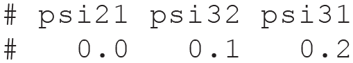
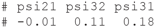
For illustration, the true parameter values are

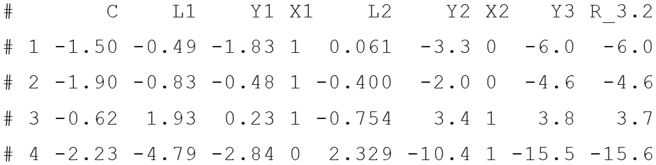
We generate a data set and display the first few rows of the data set below ⁸ :

Selecting pretreatment covariates for confounding adjustment

Before attempting to estimate each causal effect of interest, researchers must first consider putative confounding variables. This warrants selecting a set of pretreatment covariates that suffice to eliminate all noncausal associations when adjusted or statistically controlled for (Imbens & Rubin, 2015; Rosenbaum, 1984a). Extensive discussions of pretreatment confounding adjustment for causal inference have been presented elsewhere (Hernán & Robins, 2020; Morgan & Winship, 2015; Pearl, 2009; Steiner et al., 2010).

In our motivating example, an adjustment set that is sufficient to block all noncausal paths with $X_1$ and either $Y_2$ or $Y_3$ as their end points is $C_1=\{C,L_1,Y_1\}$ . Likewise, the effect of $X_2$ on $Y_3$ is unconfounded given the adjustment set $C_2=\{C,L_1,Y_1,X_1,L_2,Y_2\}$ . It is crucial to note that the covariates in each adjustment set temporally precede a focal treatment. For example, $C_2$ contains pretreatment covariates relative to $X_2$ , notwithstanding $L_2$ and $Y_2$ occurring after $X_1$ . This assumption of “no unmeasured confounding” implies that when there is no causal effect of treatment $X_t$ on outcome $Y_s,s>t$ , it can then be assumed that $X_t$ and $Y_s$ would be conditionally independent given the selected covariates in $C_t$ . Within the causal diagram in Figure 1, this assumption is represented by the absence of unmeasured common causes of treatment ( $X_1$ or $X_2$ ) and outcome ( $Y_1$ , $Y_2$ , or $Y_3$ ) and the absence of arrows between U and treatment ( $X_1$ or $X_2$ ). In this article, we assume that all confounders of the effect of each treatment $X_t$ are known and precisely measured, allowing us to estimate the causal effects of interest consistently. ⁹ Because this unconfoundedness assumption can be difficult to defend in practice, we describe a sensitivity analysis to unmeasured confounding in a later section.

A simplified g-estimation procedure

For ease of understanding, we first present a simplified version of the g-estimation procedure. It uses only regression models for the outcome given treatment and the pretreatment confounders. In a later section, we describe an enhanced version of g-estimation that is robust to biases from certain forms of incorrectly specified models and likely to be better applied in practice. Estimation proceeds by focusing on each outcome measurement in turn and sequentially estimating the treatment effects on that outcome. In particular, estimation follows a sequence starting with the latest treatment and working backward in time to the earliest treatment.

We briefly explain the motivation for such a reverse temporal ordering. The outcome $Y_3$ can be considered conceptually as the result of accumulating the effects of treatments $X_1$ and $X_2$ under the posited causal effects ${\psi }_{31}$ and ${\psi }_{32}$ , respectively. However, it is impossible to unbiasedly estimate ${\psi }_{31}$ in the presence of the time-varying confounders $L_2$ and $Y_2$ . This precludes estimating both causal effects of $X_1$ and $X_2$ on $Y_3$ using a single regression model. As we demonstrate next, in a multiple linear regression of $Y_3$ on both treatments $(X_1,X_2)$ , while controlling for the covariates $(C,L_1,Y_1,L_2,Y_2)$ , the coefficient estimator of $X_1$ will be biased for ${\psi }_{31}$ —even when no unmeasured confounding holds—because of time-varying confounding. ¹⁰ Now consider the following thought experiment. Suppose instead that $X_2$ can be assumed to have no causal effect on $Y_3$ . Then the effect of $X_1$ on $Y_3$ (that does not intersect $X_2$ ) can be estimated by appropriately adjusting for only pretreatment instances of all variables before $X_1$ and simply not adjusting for any variable causally affected by $X_1$ .

To achieve this, rather than consider the observed outcome $Y_3$ , we seek to unveil the counterfactual outcome absent the later treatment $X_2$ . To simulate this counterfactual outcome, we will “peel off” or “blip down” (Robins, 1997; Vansteelandt & Joffe, 2014) the treatment effect of $X_2$ by subtracting ${\psi }_{32}{X}_2$ from $Y_3$ for each individual. Removing the structural variation in $Y_3$ caused by the “blip” of treatment $X_2$ renders a counterfactual quantity devoid of the causal effect exerted by $X_2$ (on average). Conceptually, this step can be viewed as removing the arrow from $X_2$ on $Y_3$ in the causal diagram so that now no causal paths from $X_1$ on $Y_3$ intersect $X_2$ . The resulting counterfactual quantity, denoted by $R_{3,-x2}$ , represents a transformed outcome whose remaining structural covariation with $X_1$ (conditional on the pretreatment variables and assuming no unmeasured confounding) can be attributed to the causal effect of $X_1$ . ¹¹ We can then use $R_{3,-x2}$ in place of $Y_3$ to estimate the effect of $X_1$ on $Y_3$ (not via $X_2$ ). Crucially, only pretreatment confounders (e.g., $C,L_1,Y_1$ ) are adjusted for while excluding all posttreatment variables (e.g., $L_2,Y_2,X_2$ ). Hence, this motivates first estimating the effect of $X_2$ on $Y_3$ and then estimating the effect of $X_1$ on $Y_3$ .

Now we describe each step of the estimation procedure below:

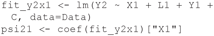
• 1. First, we estimate the Lag 1 effect of $X_2$ on $Y_3$ , parametrized by ${\psi }_{32}$ . Fit a linear regression model for $Y_3$ on $X_2$ and include the pretreatment covariates in $C_2$ . The g-estimator of ${\psi }_{32}$ is the ordinary least squares (OLS) estimator of the coefficient of $X_2$ .

• 2. We can thus use the estimate of ${\psi }_{32}$ , denoted by ${\hat{\psi }}_{32}$ , from the previous step to remove the causal effect of $X_2$ on the outcome $Y_3$ . Subtract the Lag 1 effect of $X_2$ from $Y_3$ as

$$R_{3,-x2}=Y_3-{\hat{\psi }}_{32}{X}_2.$$

Now let’s inspect the first few rows of the data set to ensure the new counterfactual quantity has been successfully created.

We can now use $R_{3,-x2}$ to estimate the Lag 2 effect of $X_1$ on $Y_3$ , which is defined as excluding any causal effect via $X_2$ .

• 3. Fit a linear regression model for $R_{3,-x2}$ on $X_1$ and include the pretreatment covariates in $C_1$ . The g-estimator of ${\psi }_{31}$ is the OLS estimator of the coefficient of X₁.

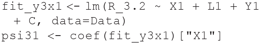
• Finally, we estimate the Lag 1 effect of $X_1$ on $Y_2$ , parametrized by ${\psi }_{21}$ . Fit a linear regression model for $Y_2$ on $X_1$ and include the covariates in $C_1$ . Note that this is the same outcome model for $R_{3,-x2}$ as in the previous step. The g-estimator of ${\psi }_{21}$ is the OLS estimator of the coefficient of $X_1$ .

Having carried out all the steps above, we can now inspect the estimates of the three causal effects below. The estimates were almost identical to the true values, with differences only at the second decimal place.

Finally, note that if we merely used the coefficient of $X_1$ in the regression model for $Y_3$ (in Step 1) as an estimator of ${\psi }_{31}$ , it would be biased, as shown below:

G-Estimation Using Lavaan

We illustrated the steps of a simplified g-estimation procedure using the linear regression functionality (lm) in R. We now describe how to carry out the above procedure using the R package lavaan (Rosseel, 2012). There are two critical advantages conferred by using lavaan for g-estimation. First, regression models for outcomes at multiple times can be evaluated simultaneously within the same lavaan model. This renders a more compact and coherent presentation of the estimation procedure. Second, equality constraints on the (regression) model parameters can be easily implemented during estimation. We provide examples of why such constraints are advantageous later.

• 1. First, we estimate both Lag 1 effects ${\psi }_{21}$ and ${\psi }_{32}$ simultaneously. We do this by fitting both linear regression models for $Y_3$ and $Y_2$ (from Steps 1 and 4 above) in the same joint model.

The g-estimators of ${\psi }_{21}$ and ${\psi }_{32}$ are then the estimators of the coefficients of $X_1$ on $Y_2$ and of $X_2$ on $Y_3$ , respectively.

• 2. Similar to Step 2 above, remove the Lag 1 effect of $X_2$ from $Y_3$ as

$$R_{3,-x2}=Y_3-{\hat{\psi }}_{32}{X}_2.$$

• 3. Similar to Step 3 above, fit a model for $R_{3,-x2}$ on $X_1$ and include the covariates in $C_1$ . The g-estimator of ${\psi }_{31}$ is the estimator of the coefficient of $X_1$ .

Having carried out all the steps above, we can now inspect the estimates of the three causal effects below. The estimates were almost identical to the true values, with differences only at the second decimal place.

Standard errors and confidence intervals can be estimated using a nonparametric percentile bootstrap procedure (Efron & Tibshirani, 1994) that randomly resamples individuals with replacement and then repeats all the above steps for each bootstrap sample. We advise against merely using the standard errors for ${\psi }_{31}$ from the fitted model in Step 3 alone because they do not adequately capture the variability in the estimates ${\hat{\psi }}_{32}$ used to determine the transformed outcome in Step 2 and may lead to biased statistical inferences.

Benefits of using constraints in lavaan

A major advantage of using lavaan for g-estimation is the ease with which parameter constraints can be introduced in the lavaan model syntax. We describe two examples relevant to g-estimation. Suppose researchers postulate a constant Lag 1 (i.e., stationary or time-invariant) effect that is equal across all treatment time points (i.e., ${\psi }_{32}={\psi }_{21}$ ). Then they merely need to add a simple line of code psi21 == psi32 to the model syntax in model_lag1 to ensure that the estimates of ${\psi }_{32}$ and ${\psi }_{21}$ are constrained to be exactly equal to each other. Alternatively, they may specify a model with the same Lag 1 effect by using the same label for the coefficients of $X_1$ on $Y_2$ and $X_2$ on $Y_3$ .

A fundamental yet empirically untestable assumption for valid causal inference is the absence of unmeasured treatment-outcome confounding. This assumption can be challenging to justify defensibly in practice, thus warranting a sensitivity analysis. Because unmeasured confounding can manifest in correlated treatment and outcome residual errors, we propose a sensitivity analysis for unmeasured confounding. We briefly summarize the steps. First, we fix the residual correlations at a given value. Next, we estimate the treatment effects under this fixed constraint. Both steps are then repeated using different fixed values of the residual correlations. This lets us systematically investigate how the effect estimates change depending on the given strength of unmeasured confounding. ¹² Stronger correlations indicate more severe violations of the unconfoundedness assumptions, whereas a zero correlation corresponds to the assumption of no unmeasured confounding.

The correlations can be readily parametrized in lavaan as follows:

A sensitivity analysis then entails fixing the residual correlations to different (nonzero) values in turn (e.g., by replacing rho in the model syntax above by a value between –1 and 1) and then carrying out the g-estimation procedure for each fixed value to gauge how different the effect estimates can be. ¹³

Doubly Robust G-Estimation

In the simplified version presented in the preceding sections, estimation was carried out using only outcome models given treatment and the pretreatment confounders. A crucial shortcoming of such an approach is that unbiased estimation is predicated on correctly specifying the statistical relations between the outcome and the covariates. ¹⁴ Hence, the estimators can be (severely) biased because of incorrectly specified outcome models. To illustrate the biases, we generated a new data set with the same values of the treatment effects but with outcomes that depended on nonlinear functions of the covariates. Using the simplified estimation procedure (i.e., with outcome models that depended linearly on main effects of the covariates) thus yielded biased estimates, as shown below:

To offer protection from this shortcoming, the estimation procedure can be supplemented with a model for the distribution of treatment to endow the g-estimators with a doubly robust property (Hernán & Robins, 2020; Kang & Schafer, 2007; Robins, 2000; Vansteelandt & Daniel, 2014). The g-estimators are unbiased when both the treatment model and the outcome model are correctly specified and consistent when either model is correctly specified (in addition to a correctly specified SNMM and unconfoundedness being satisfied). No knowledge of which model is correctly specified is required. For example (as we have done here), suppose that the outcome was generated, unbeknownst to the researcher, based on nonlinear or complex functions of the covariates. But an incorrectly specified outcome model with only main effects of the covariates is assumed for estimation. A correctly specified treatment model can ensure that the probability of the empirical estimate getting closer to the true value converges to 1 as sample size increases, thus reducing the reliance on correctly specifying the outcome model for valid statistical inference (Vansteelandt & Joffe, 2014). ¹⁵ We now describe how to carry out the doubly robust g-estimation procedure:

• 1. Fit a model for $X_1$ given the confounders in $C_1$ and a model for $X_2$ given the confounders in $C_2$ . Because treatment is binary in our simulated data set, we use a logistic regression model for each treatment. ¹⁶ This model for the treatment given the covariates is commonly termed a “propensity score” (PS; Rosenbaum & Rubin, 1983) model.

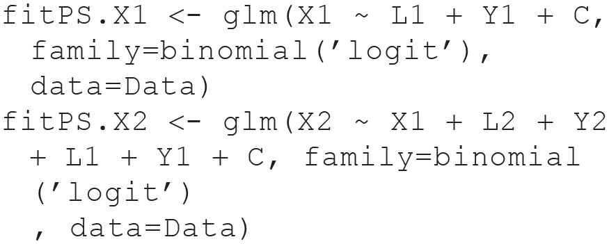
• 2. Calculate the predicted treatment or PS given the fitted models above.

Now let’s inspect the data set’s first few rows to ensure the predicted treatments have been successfully created.

• 3. Carry out the steps in the previous section but now include the predicted treatment or PS as an additional predictor in each outcome model. For example, the model for estimating the Lag 1 effects is:

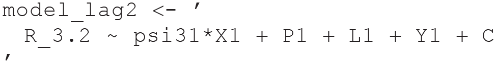
Likewise, the model for the Lag 2 effect is

Having carried out all the steps above, we can now inspect the estimates of the three causal effects below. The estimates were almost identical to the true values, with differences only at the second decimal place.

In this article, we presented a simple example of g-estimation as described in Hernán and Robins (2020, Section 21.3) and Vansteelandt and Sjölander (2016). We focused on leveraging lavaan (Rosseel, 2012) to implement g-estimation. In doing so, we hope to make g-estimation more accessible to psychology researchers who are already familiar with the features and functionalities of the widely used lavaan platform. Readers interested in alternative g-estimation procedures designed to deal with a broad variety of research settings and using other software packages or platforms as further points of investigation are referred to Picciotto and Neophytou (2016), Sterne and Tilling (2002), Tompsett et al. (2022), and Wodtke (2018); for closely related approaches, although framed slightly differently, see Ertefaie et al. (2021) and Simoneau et al. (2018). For example, g-estimation has been extended to noncontinuous outcomes, such as binary outcomes (Dukes & Vansteelandt, 2018) and time-to-event data with censored outcomes (Seaman et al., 2021; Vansteelandt and Sjölander, 2016).

Summary

Time-varying (or treatment-dependent) confounding poses unique challenges to valid causal inferences using longitudinal data. G-estimation of linear SNMMs provides a well-established solution to this problem. In this tutorial, using a linear and simple SNMM, we demonstrated how to implement g-estimation using standard parametric regression functions familiar to psychological researchers. The resulting g-estimators have a double robustness property that ensures valid inferences even under certain model misspecifications. In summary, g-estimation is flexible, practical, robust, and relatively straightforward. We encourage psychology researchers to employ g-estimation when testing the causal effects of a time-varying treatment in longitudinal studies.