Sage Journals: Discover world-class research

Abstract

Containers have become increasingly popular in computing and software engineering and are gaining traction in scientific research. They allow packaging up all code and dependencies to ensure that analyses run reliably across a range of operating systems and software versions. Despite being a crucial component for reproducible science, containerization has yet to become mainstream in psychology. In this tutorial, we describe the logic behind containers, what they are, and the practical problems they can solve. We walk the reader through the implementation of containerization within a research workflow with examples using Docker and R. Specifically, we describe how to use existing containers, build personalized containers, and share containers alongside publications. We provide a worked example that includes all steps required to set up a container for a research project and can easily be adapted and extended. We conclude with a discussion of the possibilities afforded by the large-scale adoption of containerization, especially in the context of cumulative, open science, toward a more efficient and inclusive research ecosystem.

Keywords

reproducibility containerization replication software research workflow open materials

Together with preregistration, one of the primary solutions to address the replication crisis in psychology has been to encourage open data and materials (Levenstein & Lyle, 2018). Facilitated by the rise of open-source programming languages (R, Python), free repositories (e.g., OSF, GitHub), and incentive journal policies (e.g., open science badges; Kidwell et al., 2016), the field of psychology has made important progress toward reproducible results in recent years. These incentives enable stronger foundations for future research—as of early 2019, about 35% of faculty researchers in psychology embrace open science practices compared with a mere 5% just 5 years earlier (Nosek, 2019). Yet, although necessary, sharing data and materials remains insufficient to fully ensure reproducible results (Epskamp, 2019) because results can differ significantly depending on software versions or operating systems (Glatard et al., 2015; Gronenschild et al., 2012). To alleviate these problems, it has been suggested that software version numbers and details about computing environments (e.g., operating system) should be included in the methods of scientific articles. However, obtaining previous software versions can be cumbersome, especially if the software is proprietary or relies on system dependencies (other software installed on the computer that the current software needs to work) of a specific operating system that might not be at one’s disposal.

More effective solutions have been proposed. For example, the package renv (Ushey, 2021), superseding packrat (Ushey et al., 2018), manages dependencies in R (R Core Team, 2020) by storing the source code of all R packages used in a project. These can then be recompiled for later use, which ensures consistency in R package versions across users. However, this approach does not handle system dependencies or dependencies of other programming languages and software packages. For example, the package rJava (Urbanek, 2020) needs a specific Java version to be installed on the computer; it is therefore possible that rJava works for a given user but not another—even if the project is managed by renv and operating systems are identical.

Ideally, we want to “package up” (isolate) our whole computing environment in a way that anybody on any computer can examine and replicate our work, independently of installed software, drivers, and operating systems (see Fig. 1). A popular way to achieve this goal is with virtual machines (VMs). A VM is a computer program that creates a virtual computer running inside the physical computer with its own operating system, software, and files. Using VMs, all software and their system dependencies (and sometimes scripts and/or data) used for a particular project can be bundled up and then shared with others. Yet VMs can get very large and slow, which can make sharing and using them impractical.

Fig. 1.

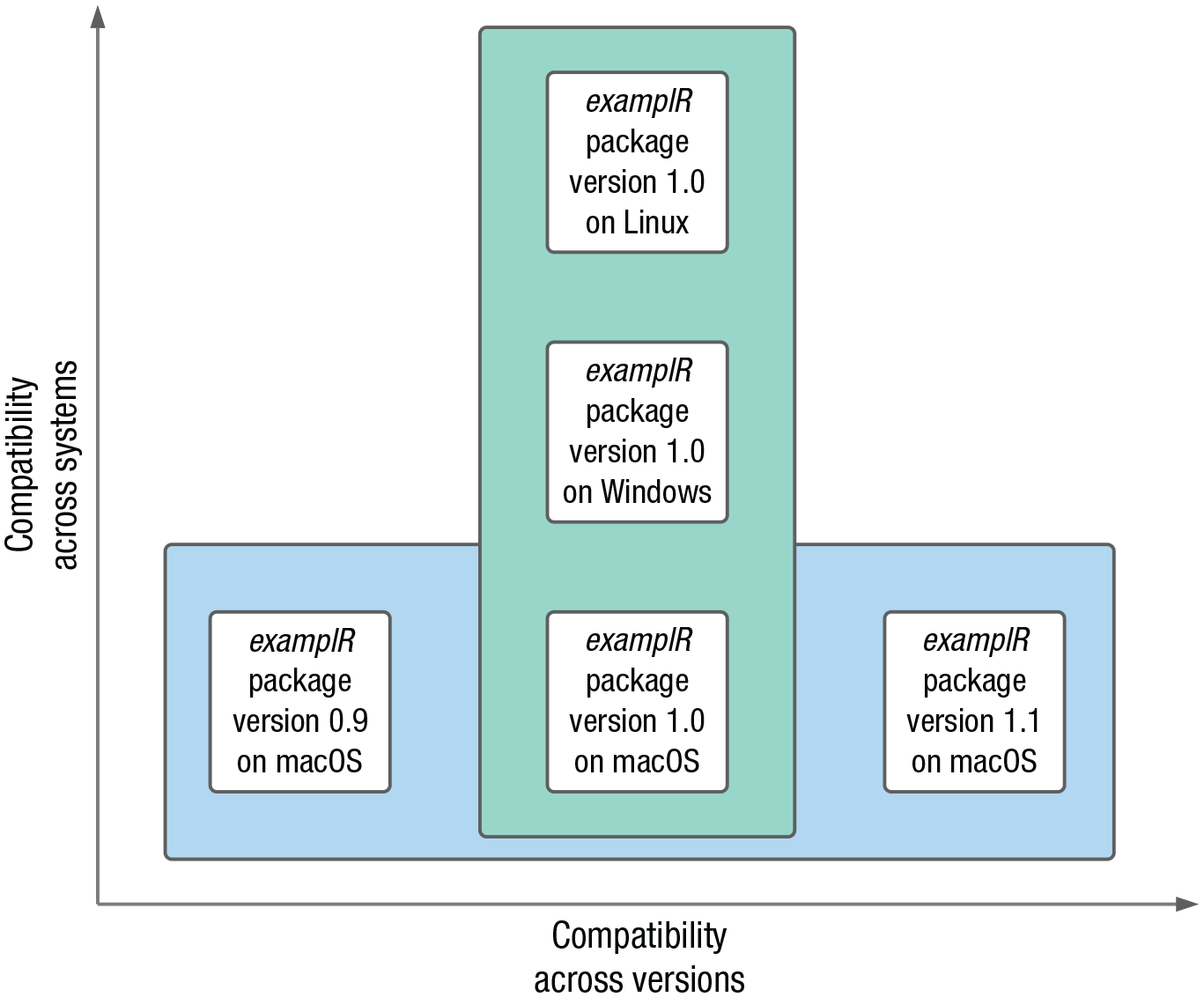
Two dimensions of compatibility enabled by containerization. Compatibility across systems relates to differences in system dependencies within or across operating systems; here, we chose to depict an example of compatibility across operating systems. Compatibility across versions relates to differences between software releases.

An alternative approach that has gained traction recently is containerization. Containers also isolate computing environments but use fewer resources than VMs. Containers are thus a lightweight alternative to VMs that make more efficient use of the underlying computing system and can more easily be shared. Originally mainly used in computer science as a way to develop and test applications in an isolated environment, containers have recently been adopted for scientific computing (Boettiger, 2015). Containerization in this context is a way to not only support reproducibility once a project is completed but also to facilitate working efficiently and collaboratively while the project is ongoing, by ensuring everything related to a research project runs smoothly and identically across all computers used across the life span of a project independently of collaborators’ individual setups.

Despite the advantages of containers and their prevalent use in fields such as computing, software engineering, and, more recently, neuroscience, containerization remains rarely used in psychology, perhaps because of a lack of awareness or because using—and especially building—containers can seem daunting for those of us lacking a computer science background. This tutorial aims to remove this barrier and demystify containerization by providing a step-by-step guide to using, building, and sharing containers within a research workflow. We use the container platform Docker and focus on the R language. After some background information on Docker, we provide an overview of basic Docker commands and of how to run R in Docker containers (Tutorial Part I: Docker Basics and the Rocker Project). In the section Tutorial Part II: Building and Sharing Personalized Docker Containers, we provide a step-by-step worked example of building, using, and sharing a personalized container for a research project. This worked example includes all required steps from start to finish and is designed to be easily adoptable and extendable by readers. We conclude with a brief summary of the tutorial and an overview of more advanced containerization workflows.

Brief Introduction to Docker

Docker (docker.com; Merkel, 2014) is an open-source containerization project based on Linux; that is, Linux is running inside the containers even though we might be on a Windows or Mac computer. Docker consists of three components: the Docker software, Docker objects, and an online Docker registry (see figure in Box 1). The Docker software consists of the Docker client and the Docker daemon. The Docker client is a command-line tool that you use to tell Docker what you want to do. When you type a command, the Docker client talks to the Docker daemon in the background, which then does all the work, such as building, running, and distributing containers. In our case, the Docker client and the Docker daemon are both on our computer, but it is possible to connect a Docker client to a remote Docker daemon.

Box 1.

Glossary of Docker Terminology

Docker engine: The containerization technology that Docker uses. The Docker engine manages containers, images, builds, and so on. It consists of the Docker daemon running on the computer and the Docker client that communicates with the daemon to execute commands.

Docker client: The command line tool that allows the user to interact with the Docker daemon.

Docker daemon: The background service running on the computer that manages Docker objects and processes, such as building, running, and distributing containers.

Dockerfile: A file containing the instructions to build a Docker image. Once the Dockerfile is set up, the docker build command can be used to build a docker image from the Dockerfile.

Docker image: The blueprint of a Docker container. Contains instructions for creating a container and defining the content, its dependencies, and the startup behavior. The docker run command creates a Docker container from the Docker image.

Docker container: A runnable instance of a Docker image. Docker containers can be created (docker run), stopped (docker stop), restarted (docker start), deleted (docker rm), or connected to storage (using the -v flag). The same container can be created and run in any environment.

Docker Hub: Registry for Docker images. Docker images can be downloaded (using docker pull) and shared (using docker push) for free on Docker Hub.

Docker ID: Username on Docker Hub.

Volumes: Used to manage data inside containers. By default, data created in a container do not persist when a container is removed. Volumes are used to give the container access to files on the computer (e.g., scripts or data) and can also be used to save files to the computer. Volumes are initialized when a container is created by using the -v flag in the docker run command.

The main Docker objects are Docker images and Docker containers. A Docker image is a read-only, unmodifiable blueprint of the desired computing environment. The image contains all instructions to create the computing environment and can be shared if others want to use the same environment. From the image, Docker can create a container—a runnable version (instance) of the image, that is, the actual computing environment that can be used to run applications or conduct analyses. An unlimited number of containers can be created from one image, and, in contrast to images, containers can be modified while running. These changes, however, are not saved back into the image. This desirable property means that each time a container is run from a particular image, it is exactly the same; you cannot “break” the image, no matter what you do in the container. If you want changes you made in the container to be saved, you need to create a new image that incorporates these changes. You can think of a Docker image as a cake recipe and the corresponding Docker container as a finished cake. The recipe contains the instructions to make the cake, it can be used to make as many cakes as you like, and it can be shared to enable others to make the same cake. Everyone using the recipe ends up with the same kind of cake, which can then be modified by adding, for instance, icing or sprinkles. However, your addition of icing and my addition of sprinkles will not change the recipe, and the next time we use the recipe, we get the same reproducible cake as before.

Finally, the third Docker component is an online repository of Docker images called Docker Hub, from which existing images can be downloaded and to which you can upload your own images if you want to share them. We illustrate all these concepts in practice throughout the tutorial, which will further clarify them. Box 1 contains additional details about the Docker architecture and definitions of Docker-related terms.

Even though other containerization platforms exist, such as CodeOcean (described in detail in Clyburne-Sherin et al., 2019) and Singularity (sylabs.io), we chose to use Docker for this tutorial for five main reasons. First, Docker is one of the leading container platforms and has been established as best practice in several research fields (Boettiger, 2015). Second, Docker runs on all major operating systems (Linux, macOS, and Windows). Third, Docker containers are easy to use, very lightweight, and fast. Fourth, Docker images can be stored and shared for free on the central registry Docker Hub. Finally, and thanks to its growing popularity, Docker benefits from a large user community and a rich ecosystem of related tools, such as Rocker (rocker-project.org; Boettiger & Eddelbuettel, 2017), which provides containers with R environments, and Neurodocker (github.com/ReproNim/neurodocker), which facilitates setting up customized containers for neuroimaging projects. Familiarity with Docker is also helpful because major tools in neighboring fields have moved to using the Docker format, such as the standardized functional MRI preprocessing pipeline fmriprep (fmriprep.org; Esteban et al., 2019). In psychology, similar trends are emerging with projects like the Experiment Factory, which allows creating Docker containers to ensure behavioral experiments can run smoothly across platforms (expfactory.github.io; Sochat, 2018).

Disclosures

All materials (Dockerfiles, data, scripts) used in this tutorial are available at osf.io/z85k3; the corresponding Docker images can be found at hub.docker.com/u/kwiebels. A wiki with commonly encountered Docker errors is also available at osf.io/z85k3. We designed this tutorial to be accessible for novices, but we do assume basic knowledge of computers (e.g., knowledge of terms such as path). If you want to learn more about basic command-line usage, see the Software Carpentry lesson on the Unix shell (swcarpentry.github.io/shell-novice). For the interested reader wanting to go beyond the material covered in this tutorial, a comprehensive general Docker guide can be found at docker-curriculum.com.

Tutorial Part I: Docker Basics and the Rocker Project

Preparations

Before starting the tutorial, go to osf.io/z85k3 and download the folder tutorial_project to a chosen location on your computer. Make a note of where you saved this folder because you will need the path to this location in the tutorial (for us, the path is /Users/kwiebels, so the path to the content of the folder is /Users/kwiebels/tutorial_project). The folder contains two files, an R script called script.R and a csv file called study2_summaryData.csv, which contains data openly available as part of a published study by our group (Wiebels et al., 2020).

Installing Docker

Docker is available for a variety of Linux distributions, for Mac, and for Windows. On Linux, you will install Docker directly; if you are on Mac or Windows, Docker is installed through Docker Desktop, an application that includes all features needed to build and share containers. To download and install Docker, follow the detailed instructions listed at docs.docker.com/get-docker in the section for your operating system. If you are using Windows, see Box 2 for Windows-specific considerations.

Box 2.

Windows-Specific Considerations

Installation

There are two ways to run Docker on Windows, either using the Hyper-V backend or using the Windows Subsystem for Linux (WSL) 2 backend (available for Windows 10 Version 1903 or higher). WSL is a full Linux kernel built by Microsoft and allows Docker containers to run natively without the need for emulation. Using the WSL 2 backend is recommended because it makes more efficient use of resources and greatly increases speed. If possible on your system, Docker will automatically select this option during the installation process (see screenshot of the Docker settings below, “Use the WSL 2 based engine” tick box). Depending on the computer setup, the WSL 2 feature on Windows might need to be enabled and the Linux kernel update package installed. Docker Desktop will alert you to this if these steps are necessary, in which case you can follow Steps 1 through 5 at docs.microsoft.com/en-us/windows/wsl/install-win10 (for further details about the WSL 2 backend, see docs.docker.com/docker-for-windows/wsl). Older versions of Windows will automatically use the Hyper-V backend (i.e., the box in the screenshot will be unticked), for which no additional steps are required.

Usage

We recommend using the Windows PowerShell. If you are using WSL 2 and prefer the WSL 2 bash terminal, you will need to prepend all commands with ‘sudo.’

Paths

Paths in Windows are different from the ones on Linux and Mac (which is used in this tutorial), so you will need to adapt the paths slightly. If your path is C:\Users\kwiebels\tutorial_project, for example, you need to change it to /c/Users/kwiebels/tutorial_project. If you are using the WSL 2 bash terminal, the path needs to be changed to /mnt/c/Users/kwiebels/tutorial_project.

Running Docker containers

Once Docker is installed, it is time to launch it! You should see the Docker icon in the taskbar, indicating that Docker is running. Docker is then accessible from the terminal (on Mac, open the terminal by opening the Applications folder, then opening Utilities and double-clicking on Terminal; on Windows, open the PowerShell by clicking Start, typing PowerShell, and then clicking Windows PowerShell). Once a terminal window is open, you can type commands and execute them using the return/enter key.

The general syntax for running a Docker container is:

An IMAGE, from which the container is derived, must be specified; the rest of the terms are optional. OPTIONS can be used to constrain the container’s behavior; we describe a range of them throughout the tutorial. The TAG instructs Docker to use a specific version of an image, and finally, the COMMAND tells Docker which command to execute when the container starts. Most of the time, the Docker image developer specifies this start-up behavior (e.g., a typical command of an R container is simply to start R), but it can be overridden, for example to get the R version instead of starting R (R –version) or to run an R script that reproduces all analyses used in an article (e.g., Rscript run_all.R).

To test your Docker installation, open a terminal window and run the line below:

If your installation works correctly, you should see the text output shown in Figure 2.

Fig. 2.

Screenshot of the hello-world container output.

If you see this output, you just ran your first Docker container! The container is called hello-world and is not overly useful—it does not do anything beyond printing text. The image from which the container was created is stored on—and was downloaded from—Docker Hub (you can look at the hello-world Docker image online at hub.docker.com/_/hello-world). docker run automatically downloads (pulls) Docker images from Docker Hub if they cannot be found locally (i.e., on your computer). You can also explicitly do this by running docker pull hello-world (which pulls the image from Docker Hub) before docker run hello-world (which creates a container from the image and runs it).

Once you have downloaded a Docker image, you can run

to get a list of Docker images available on your computer. You will see the hello-world image along with a tag (version), the ID of the image, and its creation date and size (see Fig. 3).

Fig. 3.

Screenshot of the docker images command output.

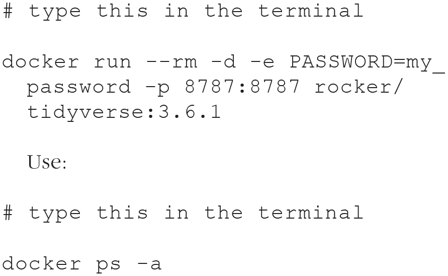
In addition to a list of images, you can also get a list of all containers on your computer using

The -a flag means that all containers will be displayed, independent of their status (a flag is an option appended to a command; for a list of all available flags for docker ps, type docker ps –help or check the documentation online at docs.docker.com/engine/reference/commandline/ps). You should see a list of all containers you have created so far as well as additional information about each container—including the container ID, the name of the corresponding image, and the container’s status (see Fig. 4).

Fig. 4.

Screenshot of the docker ps -a command output.

The container’s status indicates for how long the container has been running or how long ago it was stopped (exited). Some containers stop automatically (as was the case with the hello-world container), but some have to be stopped manually.

By default, after a container is stopped, it is not removed from the computer, and every time you use docker run, a new container is created. This means that if you run docker run hello-world again, you will end up with two hello-world containers on your computer. Keeping all created containers on your computer unnecessarily takes up disk space given that we typically create a new container for each use to start with the same clean environment. The only thing we need to keep is the image, from which a new container can be created any time. To remove an existing container, use the following command, replacing <container_ID> with the container ID from the docker ps -a output (e.g., 796e9ec1e334 for the hello-world container in our case):

Note that you can copy and paste the container ID instead of having to write it out manually (in the terminal on Mac, copying and pasting works as usual; in the Windows PowerShell, highlight what you want to copy and use right click to paste). To remove all containers from your computer at once, the shortcut docker rm $(docker ps -a -q) can be used (see Box 3 for a list of other useful Docker commands).

Box 3.

Glossary of Common Docker Commands

docker pull <image_name> downloads an image from DockerHub.

docker run <image_name> runs a container.

docker run -it <image_name> runs a container interactively.

docker run –rm -it <image_name> is the same as above but causes the container to be removed after it has been stopped.

docker run –rm -it -v <path_on_computer>:<path_in_container> <image_name> additionally mounts a local folder into the Docker container (in this case, <path_on_computer> is mounted into the container and is accessible in the container under <path_in_container>).

docker exec -it <container_id> bash opens a terminal inside a running Docker container (e.g., to install additional libraries in a container that is already running).

docker build -t <image_name> . builds a Docker image called <image_name> in the current folder.

docker images or docker image ls returns a list of all Docker images stored on the computer.

docker ps or docker container ls returns a list of currently running containers.

docker ps -a returns a list of currently running and stopped containers (i.e., all created containers).

docker stop <container_ID> stops a running container.

docker start <container_ID> restarts a stopped container.

docker rm <container_ID> removes a stopped container.

docker rm $(docker ps -a -q) is a shortcut to remove all stopped containers.

docker rmi <image_ID> removes an image.

docker rmi $(docker images -a -q) is a shortcut to remove all images.

To avoid having to manually remove containers, it is possible to specify at the time a container is created that the container should be removed automatically after it is stopped. This is achieved with the –rm flag:

This time, the container was automatically removed from the computer after exiting. Note that if you use Docker Desktop, you can also start, stop, and remove containers and images in the Docker Desktop interface.

The Rocker project

Thanks to the Rocker project (rocker-project.org), running R inside a Docker container is just as easy. Rocker maintains Docker images with R or RStudio preinstalled, which means that we do not have to create R Docker images from scratch. There are different images suited for different needs (see all images at hub.docker.com/u/rocker). Some images only include R or RStudio, whereas others already have some R packages preinstalled, for example the rocker/tidyverse image, which includes the tidyverse (Wickham, 2017), devtools (Wickham & Chang, 2016), and remotes (Hester et al., 2019) packages, or rocker/ml, which includes common machine learning packages.

Rocker base R containers

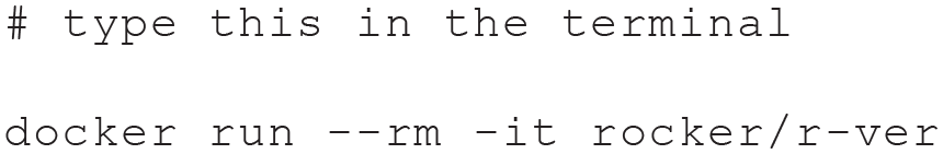
To run a container with a base R environment, simply type the line below:

rocker/r-ver here refers to the image r-ver in the repository of the Docker Hub user rocker. In the terminal, you should see R start, but then exit again straight away. This happens because to interact with R, you need to use the -it flag. The -it flag lets you interact with the R console in the terminal; that is, you can use the keyboard to provide inputs, and outputs are returned to the terminal. Change the above command to

An interactive R session is now running in Docker (see Fig. 5), and you can use R as you usually would. For example, typing mean(c(2,4)) will return 3. When you are done, type q() to quit the R session, stop the container, and get back to the terminal.

Fig. 5.

Screenshot of an interactive base R session in Docker running in the terminal.

By default, Docker pulls and runs the latest version of an image from Docker Hub. At the time of writing, the latest Rocker image uses R version 4.0.4 (see Fig. 5). When Docker is used for reproducibility reasons, a versioned—instead of the latest—image should be used to ensure that everyone using the container will get the same R version independently of when the container is created. To use a specific R version, tags can be specified. To use R version 3.6.1, for instance, the previous command needs to be adapted as follows:

Rocker RStudio containers

Rocker also maintains RStudio images, which might provide a more comfortable analysis environment than accessing R through the command line. These containers run an instance of RStudio server, which can be accessed from—and interacted with—a web browser. As with the base R container, you can choose the R version you want to use. Running the following command will start an RStudio container with R version 3.6.1 (note that the command has to be written on one line):

There are three additional flags this time. The -d flag means that the container will run in the background (detached) so that the terminal can still be used for other commands. The RStudio server instance needs a username (rstudio by default) and a password, set using the environment variable PASSWORD with -e PASSWORD=my_password. We have chosen my_password for this example, but this can be changed to any password you want. -p 8787:8787 maps a port from inside the container to the computer (in the form of -p <port_computer>:<port_container>). A port enables communication between the computer and anything connected to the Internet, in this case the RStudio server. To enable the connection to RStudio server, RStudio is assigned a port number inside the container. Given that the container is isolated from the rest of your computer, this port number needs to be passed from inside the container to the computer so that RStudio can be accessed from a Web browser outside the container.

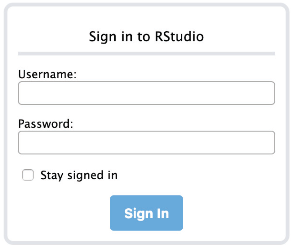
After typing the command, Docker will print the container ID to the terminal. To use the containerized RStudio, open a browser window and enter localhost:8787 as the URL. You will be redirected to a login page (see Fig. 6) and prompted to enter the username (rstudio) and the password you set (my_password unless you changed it).

Fig. 6.

Screenshot of the RStudio server login screen.

Upon login, you will be running RStudio in the browser (see Fig. 7). This RStudio instance can be used just like RStudio running locally on your computer. To quit the session, click the red button on the top right and close the browser tab.

Fig. 7.

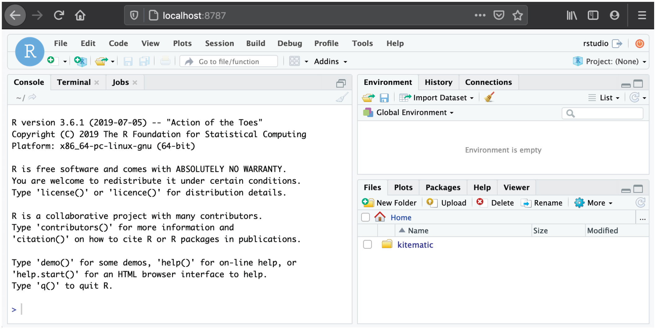
Screenshot of an RStudio session running in Docker.

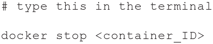
When you are done, you need to stop the Docker container manually in the terminal because it will still be running in the background (because of the -d flag in the initial docker run command). Get the container ID with docker ps -a and type the following command, replacing <container_ID> with the ID of the RStudio container:

Once stopped, the container is automatically removed because we used the –rm flag in our initial command. You can confirm this using docker ps -a.

Accessing files in Docker containers

By default, Docker does not have access to any files on the computer; however, we might want to load a local data set or write results to a specified folder on the computer. To give access to a local folder, the -v (volume) flag is used in the docker run command along with details about which folder on your computer you want to access and the location inside the container at which you want the folder to be available (the format for this is <path_on_computer>:<path_in_container>).

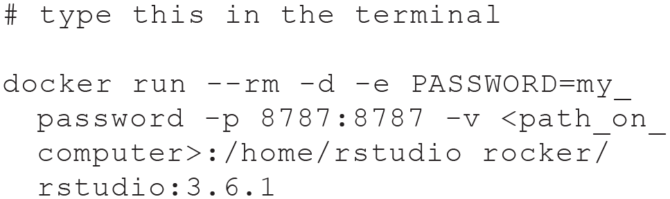
The command below will map the folder at <path_on_computer> to the path /home/rstudio inside the Docker container (/home/rstudio is the default working directory inside RStudio Rocker containers, so this is the folder in which you land when you open RStudio). Replace <path_on_computer> with the path to the folder on your computer that you downloaded for this tutorial (e.g., /Users/kwiebels/tutorial_project). If you are using Windows, you will need to adapt the path slightly to make it work in the Linux environment inside the container (see Box 2):

After running the command, open RStudio in the browser, as before. You should now see the content of the folder in the RStudio Files tab (see Fig. 8). Remember to stop the container when you are done using docker stop <container_ID>.

Fig. 8.

Screenshot of an RStudio session with access to a local folder.

If your research project does not require packages beyond the ones provided by Rocker, you can use one of the Rocker images without any modifications. If you need additional packages—which will likely be the case—it is possible to install them in RStudio while the container is running. The problem with this approach, however, is that the packages need to be reinstalled every time a new container is created, which also means that they will not be available automatically for other researchers who use your container. To build a personalized computing environment that can be used and shared with collaborators and other researchers, you can build your own Docker image with all required packages. That way, the packages will automatically be available in each container that is created from the image. In the following section, we provide a worked example of how to create and use a personalized container and how to share it. The guide includes all required steps so that it can easily be adopted and extended for your own research.

Tutorial Part II: Building and Sharing Personalized Docker Containers

In this section, we aim to provide a step-by-step guide on how to build, use, and share a personalized container for your research project. Building a personalized container involves several steps but is a straightforward process, especially if only R is required. In the following sections, we demonstrate how to (a) build your own personalized Docker container with RStudio and additional R packages; (b) load a local data set inside your personalized container, create summary statistics and a plot, and write results to a local folder; and (c) make the container available on Docker Hub or OSF (osf.io).

Building a personalized Docker container

Building a personalized container involves two main steps. We first need to write a Dockerfile—a file with a set of instructions in which we specify everything that we want to include in the container. This Dockerfile is then used to build a Docker image, from which we can then run containers.

For this example, we want to build an RStudio container with R version 3.6.1 and use the R packages psych (Revelle, 2011), ggplot2 (Wickham, 2011), and gghalves (Tiedemann, 2020) to generate summary statistics and a plot. As described previously, thanks to the Rocker project, we do not need to build our container from scratch, which would involve installing R on the Linux system inside the container. Instead, we can simply use a suitable Rocker image as a starting point and then add the packages we need. Given that we need ggplot2, which takes quite a long time to install, and remotes (Hester et al., 2019) to install gghalves from GitHub, we will start with the rocker/tidyverse:3.6.1 image, which has both packages preinstalled.

To start building your container, open the terminal and move into the tutorial_project folder (replace <path_to_folder> with your path):

You can check that you are in the right location by typing pwd (print working directory). Next, create a file called Dockerfile in that folder. This file needs to have that specific name and must not have an extension, such as “.txt,” otherwise the building process will fail. On Linux/Mac, use

On Windows, use

The general format of a Dockerfile is

Instructions do not have to be capitalized, but it is convention to do so. A Dockerfile must start with a FROM <image_name> statement that specifies which Docker image is used as the base image (i.e., which Docker image will be extended; in our case, the Rocker tidyverse image). Other common instructions include COPY (copies files from the computer into the container), ENV (sets an environment variable), and RUN (runs a command). See the Dockerfile reference (docs.docker.com/engine/reference/builder) for a full list. In our example, we just want to add some R packages, so we only need the FROM and RUN instructions. Note that although the COPY instruction can be used to include scripts and data in the image, it is preferable to load these files into the container at runtime so that the size of the image does not increase drastically and sensitive data are not accidentally included in and distributed with the image (for general advice on writing Dockerfiles, see Nüst et al., 2020).

For our Docker container, we are going to start with a versioned Rocker tidyverse image. Open the Dockerfile using your favorite text editor, and add the following line:

After this line, we need to specify which additional R packages we want to install. Before adding this information to the Dockerfile, it is usually a good idea—that can save a lot of time—to test installing the packages first. Most packages should install without any issues, but some packages rely on system libraries that have to be installed first and will throw an error at first try. These errors can be challenging to track down if they are encountered only while building the Docker image. To test the installations, we run a container of the tidyverse image and then—instead of opening RStudio—open a terminal inside the running container. This way, we can install the packages from the command line to ensure those commands will work in the Dockerfile.

A running container can be accessed using the docker exec command, as shown below. First, start a container of the tidyverse image you specified in the Dockerfile:

to get the ID of the running container and type:

Bash is the command language used by the terminal in this container. The command will open a terminal inside the container (see Fig. 9). In this case, root is the user, and 160ed3f1f63c is the ID of the running container.

Fig. 9.

Screenshot of a bash prompt inside a running container.

In the terminal inside the container, you can try out installing the packages you need. Running

will use R’s install.packages() function to install the psych package.¹ The -e flag specifies that the input is an expression that will be evaluated. Given that these are normal R commands, you can do anything you usually do, for example, install a certain package version using the devtools package. The process should finish without errors. Once the psych package has been installed, it will become available in the dockerized RStudio in your browser, and you will be able to load and use it as usual. The process for gghalves is slightly different because it is not available on CRAN (The Comprehensive R Archive Network) and therefore needs to be installed from GitHub. Rocker’s helper function installGithub.r that is available inside the container can be used to achieve this:

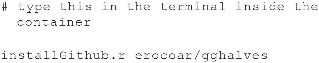
Once those two packages have installed successfully, you can safely add them to the Dockerfile using RUN instructions:

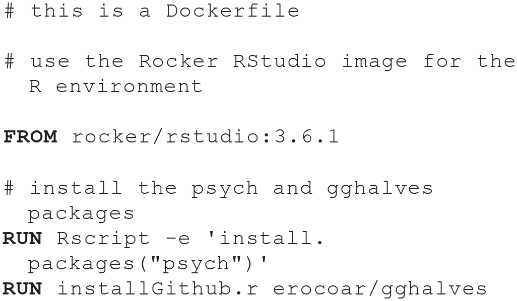
After saving this Dockerfile, exit the terminal inside the Docker container by typing exit, and stop the running RStudio container with docker stop <container_ID>. It is now time to build the Docker image:

-t lets us specify a name for our Docker image (we chose tutorial_project here) and optionally a tag (by default latest is used), and . indicates that the Docker image should be built in the current folder (this needs to be specified so that Docker knows where the Dockerfile is). If you get an error here, make sure you are in the right folder in the terminal, otherwise the Dockerfile will not be found. Depending on your computer, the building process might take a few minutes. Once the Docker image is built, we can use it for analyses, which we show in the next section.

Using the container

Having set up the container, we can now use it to load a data set, compute summary statistics, create a plot, and save the output in a folder on the computer. By now, you are familiar with how to run a container; all that is needed is to replace the image name with the name you gave your personalized Docker image. We use the script and the data you downloaded from OSF, so you need to give Docker access to the folder that contains these downloaded files (replace <path_on_computer> with the path to that folder):

You are now running your first personalized container! After opening RStudio in the browser, you will see the data file (study2_summaryData.csv) and the R script (script.R). You will also see that the packages psych, ggplot2, and gghalves are available.

When looking at the script, you will see that it loads some packages, computes summary statistics using the psych package, creates a plot using ggplot2 and gghalves,² and saves the results in a file. Run the script as you usually would in RStudio, and you will see two new files being created, descriptives.csv and plot_difficulty.png. These files are saved in the folder on your computer that you specified in the command above (the same folder that contains the script and the data), which means that you have access to those files even after stopping and removing the container. Once you have run the script, you can close RStudio and stop the container using the docker stop command.

In some situations, you—or others—might just want to run the container to reproduce and inspect the results instead of interacting with the data or code inside the container. In this case, a slightly adapted command can be used to start the container, run the script, save the output, and then exit and remove the container:

Sharing the container

When you have created and used a personalized container for a research project, you might want to share it, along with the scripts and data, with your collaborators while the project is ongoing or upon completion of the project to make your analysis reproducible for other researchers. Docker containers can be shared either by uploading the Docker image to Docker Hub so that others can download it or by sharing the Dockerfile on a repository such as OSF so that others can build the corresponding Docker image themselves. We demonstrate both options in the next two sections.

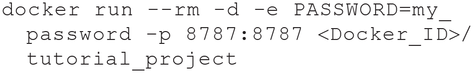
It is good practice to include usage instructions for the container in the Dockerfile and/or in a README file. To do this, open the Dockerfile and add the following information at the bottom of the file:

Sharing the Docker image on Docker Hub

To share the image on Docker Hub, you will need to create a free Docker Hub account. To do this, go to hub.docker.com, click on “Sign up,” and fill out the information. Once your account is created, return to the terminal and log in with your credentials:

For Docker to know to which repository on Docker Hub to upload your image, you need to tag your image with your Docker ID (the username you used when creating the account on Docker Hub) and the image name in the following format:

The image name can remain the same. Given the example above, this would be

You can then upload (push) the container to Docker Hub:

It is important here to use the format <Docker_ID>/<image_name> so that Docker knows where on Docker Hub to publish. Once the image is on Docker Hub, others can easily download and run it using

Sharing the Dockerfile on OSF

If you prefer sharing the Dockerfile on OSF, along with any materials or data you want to share, you can achieve this very easily. If you have never used OSF before to share project-related files, follow Soderberg’s (2018) guide. All that is left to do once the OSF repository is set up is to upload the Dockerfile into that repository. Others can then download that Dockerfile and use the docker build command to build the corresponding Docker image.

These two approaches can also be combined because they both have advantages. Sharing the image on Docker Hub makes it easier for others to download and use it because they do not need to build the image themselves. Sharing the Dockerfile itself has the advantage that others can inspect the file to see exactly what is included and adapt it for their own purpose if desired. Note that there is a slightly more advanced way to upload Docker images to Docker Hub, which will automatically make the Dockerfile available as well (see Box 5, Automated Builds Using GitHub).

Once you have finished the tutorial, you might want to delete all containers and images we used throughout because they can take up quite a lot of disk space. Use the following two commands to achieve this:

Discussion

In this tutorial, we explained the basics of containerization and provided step-by-step guides for building, using, and sharing Docker containers. The first part of the tutorial introduced basic Docker commands and the Rocker project as a way to run R code in containers. In the second part of the tutorial, we showed how to set up a personalized container for a research project, from writing a Dockerfile to sharing the Docker image.

Containerization is an important step toward making research reproducible by providing a consistent computing environment that can be used by all collaborators over the course of a project and that can be shared along with the publication. Throughout the tutorial, we focused on the R language, but we provide a resource below for setting up a Python environment to illustrate the process for projects that require tools beyond R. We aimed to provide a resource that can be easily adapted and extended to one’s own research projects or workflows. Below, we summarize some Docker uses that are beyond the scope of this tutorial but might be of interest to some readers before concluding the tutorial with some general remarks.

Additional steps

Integrating containerization into the research workflow

Sharing a container after a research project has been finalized ensures that your analyses are reproducible. However, containerization can also greatly benefit your collaborators—and yourself—throughout the development of the project by making sure that code does not break over time and that every collaborator works in exactly the same environment without the need to synchronize all pieces of software manually. This aspect might be especially beneficial for collaborators who are not heavily involved in the data analysis part of the project and need to inspect the results only from time to time or give feedback.

Figure 10 depicts an example workflow with containers being used as the computing environment from the start of a research project. At the beginning of the project (purple box), a shared location (e.g., a network drive) is set up where the data and all analysis scripts will be stored (blue box). A Dockerfile for the anticipated computing environment is also created. Using the Dockerfile, a Docker image is built, which is then shared on Docker Hub. From there, all collaborators download the Docker image and use it as the computing environment for the duration of the project. 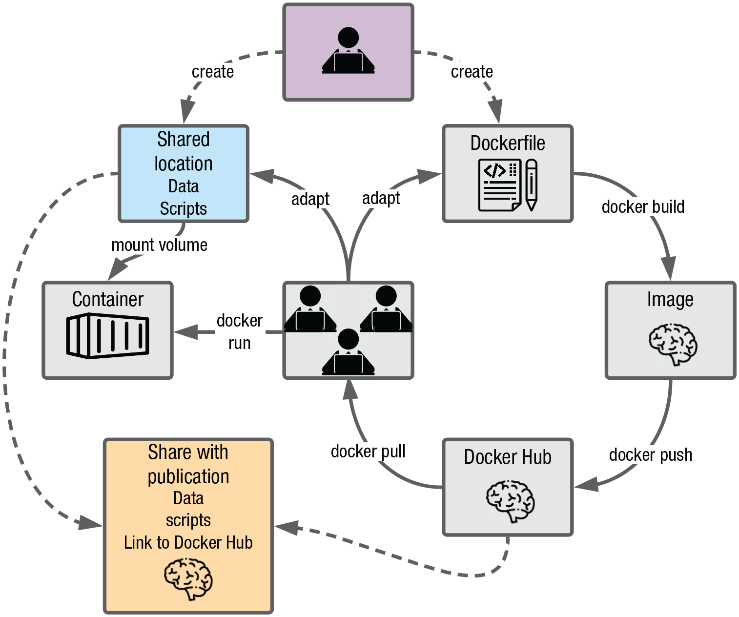Given that the Dockerfile might have to be adapted from time to time (e.g., to make additional packages available), the docker pull command with the tag latest can be used before running the container. The latest tag checks for updates to the image and downloads the newest version if necessary, which means that all collaborators automatically run the most up-to-date container (note that the run command with the latest tag does not check for updates). Using the -v flag in the docker run command will make the files available in the container and ensure that changes made in the container will be saved. At the end of the project, the final versions of the data, scripts, and the Docker container (in the form of a link to Docker Hub or, alternatively, the Dockerfile itself) are then shared alongside the publication (see orange box).

Fig. 10.

Example research workflow using containerization.

More advanced containers and workflows

The image we have built in this tutorial is relatively simple; it includes only R and a few packages. We chose this example to be accessible and easily extendable to suit your purpose. However, some projects require analysis tools beyond R. For instance, if you have electroencephalography (EEG) data and want to use MNE-Python (Gramfort et al.,2013, 2014) in addition to R for data processing and analysis, an R container needs to be extended with a Python environment and the right Python tools need to be installed. We show an example of a Dockerfile for this advanced scenario in Box 4 and provide a step-by-step guide for building this container at osf.io/z85k3.

Box 4.

Docker Containers Beyond R

Sometimes, languages beyond R are required for data analysis. For this example, we want to build a Docker container with RStudio, Python (Version 3.6 or higher), the mne Python package, and the reticulate (Allaire et al., 2018) and mne (Engemann, 2020) R packages.

An example Dockerfile for this scenario is shown below. See osf.io/z85k3 for a step-by-step guide.

# this is a Dockerfile

# use the Rocker tidyverse image for the R environment

FROM rocker/tidyverse:3.6.1

# update Debian package manager

RUN apt-get update

# install Anaconda

RUN echo ‘export PATH=/opt/conda/bin:$PATH’ > /etc/profile.d/conda.sh && \

wget –quiet https://repo.anaconda.com/archive/Anaconda3-2020.07-Linux-x86_64.sh -O ~/anaconda.sh && \

/bin/bash ~/anaconda.sh -b -p /opt/conda && \

rm ~/anaconda.sh

# set Python path

ENV PATH /opt/conda/bin:$PATH

# configure reticulate to point to the conda Python executable

RUN echo “RETICULATE_PYTHON_ENV=/opt/conda/bin” >> /usr/local/lib/R/etc/Renviron

# install MNE

RUN pip install mne

# install reticulate and MNE-R

RUN Rscript -e ‘install.packages(“reticulate”)’

RUN Rscript -e ‘devtools::install_github(“mne-tools/mne-r”)’

Beyond more elaborate containers, there are also a number of additional, more advanced features that can be integrated within the containerization workflow. These are not covered in depth here for simplicity purposes; however, interested readers may refer to Box 5 for examples of more advanced setups and corresponding resources.

Box 5.

Advanced Docker Workflows

There are several more advanced ways Docker can be used to facilitate the reproducibility of the research workflow. Here, we highlight two important ones: automated builds using GitHub and containerization beyond computing environments.

Automated Builds Using GitHub

The Docker build process can be automated by storing the Dockerfile in a GitHub repository and by linking this GitHub repository to Docker Hub. The Docker Hub repository can then be configured such that every time the Dockerfile on GitHub is updated, an updated Docker image is automatically built, tested, and pushed to Docker Hub. Automatic builds therefore render the manual build and push steps in Figure 10 redundant, which is especially useful if the Dockerfile is anticipated to change frequently throughout the project. See docs.docker.com/docker-hub/builds for a guide on how to set up automated builds and Vuorre and Curley (2018) for a tutorial on Git and GitHub.

Containerization Beyond Computing Environments

Although the focus of this tutorial is on containerization for the data analysis part of a research project, Docker can facilitate incorporating other parts of the research process into a reproducible workflow, including running experiments and reporting results.

The Experiment Factory (Sochat, 2018) facilitates creating Docker containers for behavioral experiments. Containerizing experiments ensures that they can be run anywhere and on any computer and that they can easily be shared. This is likely especially useful for decentralized research projects, which are run by several labs, to minimize problems with the setup and compatibility issues. See expfactory.github.io for further details.

Reproducible reporting can be achieved with the R package liftr (Xiao, 2019), which uses Docker to containerize and render RMarkdown documents. An RStudio addin is available to facilitate this process. See liftr.me for further details. See also Peikert and Brandmaier (2019) for a suggested comprehensive workflow, including version-controlled data management, dependency management using Makefiles, containerized computing environments using Docker, and dynamic document generation using RMarkdown.

Concluding remarks

Containers are important components to increase reproducibility, but the advantages of containerization have more widespread ramifications: They facilitate collaboration, especially across global research groups, enabling efficient workflows with a common template of the research project. Another exciting prospect brought about by containers is that of truly cumulative science—sharing practices such as open data and materials have helped shape incremental research tremendously, yet cumulative science can still be hindered by compatibility and dependency issues. Containerization is the next step in that process to ensure robustness across users and time and facilitate secondary data analysis (Weston et al., 2019).

Finally, and beyond advancing scientific research, investing time and effort in learning and working with containers may be a wise professional move for researchers, especially at early stages of a career. This idea perhaps seems to run against mainstream thinking about the cost associated with open practices, especially for early career researchers (C. Allen & Mehler, 2019; Nosek et al., 2012; Poldrack, 2019). Yet given job prospects in research and academia, many researchers may likewise question whether in-depth, systematic knowledge about very specific aspects of psychological science remains valuable or, at the very least, transferable. Thorough expertise on the validity of a specific scale, construct, or paradigm may not generalize well to another professional workplace; in contrast, computational or software skills such as fluency in one or more programming languages (e.g., R, Python) or a practical understanding of version control or containerization (e.g., git, Docker) can easily generalize to professional settings outside of academia. In this context, proficiency with containerization, among the broader set of computational tools required of a modern scientist, may prove to be a worthwhile investment for psychological scientists at all career stages.

Footnotes

Acknowledgements

We thank Matti Vuorre, Erin M. Buchanan, and two anonymous reviewers for their constructive and helpful feedback throughout the reviewing process. We also thank Ding-Cheng Peng and Lenore Tahara-Eckl for comments and feedback on an earlier version of this tutorial.

Transparency

Action Editor: Daniel J. Simons

Editor: Daniel J. Simons

Author Contributions

K. Wiebels and D. Moreau developed the idea for the article and wrote the manuscript. Both authors approved the final manuscript for submission.

ORCID iDs

Kristina Wiebels

David Moreau

Notes

References

Allaire

J. J.

Ushey

Tang

Eddelbuettel

Lewis

Geelnard

(2018). Reticulate: Interface to ‘Python.’ R Package Version, 1(8). https://github.com/rstudio/reticulate

Allen

Mehler

D. M. A.

(2019). Open science challenges, benefits and tips in early career and beyond. PLOS Biology, 17(5), Article e3000246. https://doi.org/10.1371/journal.pbio.3000246

Allen

Poggiali

Whitaker

Marshall

T. R.

Kievit

(2018). Raincloud plots: A multi-platform tool for robust data visualization (No. e27137v1). PeerJ Preprints. https://doi.org/10.7287/peerj.preprints.27137v1

Boettiger

(2015). An introduction to Docker for reproducible research. Association for Computing Machinery, 49(1). https://doi.org/10.1145/2723872.2723882

Boettiger

Eddelbuettel

(2017). An introduction to Rocker: Docker containers for R. The R Journal, 9(2), 527–536.

Clyburne-Sherin

Fei

Green

S. A.

(2019). Computational reproducibility via containers in psychology. Meta-Psychology, 3. https://doi.org/10.15626/mp.2018.892

Engemann

(2020). mne: Fast access to MNE-Python from within R. https://github.com/mne-tools/mne-r

Epskamp

(2019). Reproducibility and replicability in a fast-paced methodological world. Advances in Methods and Practices in Psychological Science, 2(2), 145–155.

Esteban

Markiewicz

C. J.

Blair

R. W.

Moodie

C. A.

Isik

A. I.

Erramuzpe

Kent

J. D.

Goncalves

DuPre

Snyder

Oya

Ghosh

S. S.

Wright

Durnez

Poldrack

R. A.

Gorgolewski

K. J.

(2019). fMRIPrep: A robust preprocessing pipeline for functional MRI. Nature Methods, 16(1), 111–116.

10.

Glatard

Lewis

L. B.

Ferreira

Silva

Adalat

Beck

Lepage

Rioux

Rousseau

M.-E.

Sherif

Deelman

Khalili-Mahani

Evans

A. C.

(2015). Reproducibility of neuroimaging analyses across operating systems. Frontiers in Neuroinformatics, 9, Article 12. https://doi.org/10.3389/fninf.2015.00012

11.

Gramfort

Luessi

Larson

Engemann

D. A.

Strohmeier

Brodbeck

Goj

Jas

Brooks

Parkkonen

Hämäläinen

(2013). MEG and EEG data analysis with MNE-Python. Frontiers in Neuroscience, 7, Article 267. https://doi.org/10.3389/fnins.2013.00267

12.

Gramfort

Luessi

Larson

Engemann

D. A.

Strohmeier

Brodbeck

Parkkonen

Hämäläinen

M. S.

(2014). MNE software for processing MEG and EEG data. NeuroImage, 86, 446–460.

13.

Gronenschild

E. H. B. M.

Habets

Jacobs

H. I. L.

Mengelers

Rozendaal

van Os

Marcelis

(2012). The effects of FreeSurfer version, workstation type, and Macintosh operating system version on anatomical volume and cortical thickness measurements. PLOS ONE, 7(6), Article e38234. https://doi.org/10.1371/journal.pone.0038234

14.

Hester

Csárdi

Wickham

Chang

Morgan

Tenenbaum

(2019). remotes: R package installation from remote repositories, including “GitHub.” https://CRAN.R-project.org/package=remotes

15.

Kidwell

M. C.

Lazarević

L. B.

Baranski

Hardwicke

T. E.

Piechowski

Falkenberg

L. -S.

Kennett

Slowik

Sonnleitner

Hess-Holden

Errington

T. M.

Fiedler

Nosek

B. A.

(2016). Badges to acknowledge open practices: A simple, low-cost, effective method for increasing transparency. PLOS Biology, 14(5), Article e1002456. https://doi.org/10.1371/journal.pbio.1002456

16.

Levenstein

M. C.

Lyle

J. A.

(2018). Data: Sharing is caring. Advances in Methods and Practices in Psychological Science, 1(1), 95–103.

17.

Merkel

(2014). Docker: Lightweight Linux containers for consistent development and deployment. Linux Journal, 2014(239), Article 2. https://www.linuxjournal.com/content/docker-lightweight-linux-containers-consistent-development-and-deployment

18.

Nosek

B. A.

(2019, June 6). The rise of open science in psychology, a preliminary report. https://cos.io/blog/rise-open-science-psychology-preliminary-report/

19.

Nosek

B. A.

Spies

J. R.

Motyl

(2012). Scientific Utopia: II. Restructuring incentives and practices to promote truth over publishability. Perspectives on Psychological Science, 7(6), 615–631.

20.

Nüst

Sochat

Marwick

Eglen

S. J.

Head

Hirst

Evans

B. D.

(2020). Ten simple rules for writing Dockerfiles for reproducible data science. PLOS Computational Biology, 16(11), Article e1008316. https://doi.org/10.1371/journal.pcbi.1008316

21.

Peikert

Brandmaier

A. M.

(2019). A reproducible data analysis workflow with R Markdown, Git, Make, and Docker. PsyArXiv. https://doi.org/10.31234/osf.io/8xzqy

22.

Poldrack

R. A.

(2019). The costs of reproducibility. Neuron, 101(1), 11–14.

23.

R Core Team. (2020). R: A language and environment for statistical computing. R Foundation for Statistical Computing.

24.

Revelle

(2011). An overview of the psych package. Department of Psychology, Northwest University.

25.

Sochat

(2018). The Experiment Factory: Reproducible experiment containers. Journal of Open Source Software, 3(22), Article 521. https://doi.org/10.21105/joss.00521

26.

Soderberg

C. K.

(2018). Using OSF to share data: A step-by-step guide. Advances in Methods and Practices in Psychological Science, 1(1), 115–120.

27.

Tiedemann

(2020). gghalves: Compose half-half plots using your favourite geoms. https://CRAN.R-project.org/package=gghalves

28.

Urbanek

(2020). rJava: Low-level R to Java interface. https://CRAN.R-project.org/package=rJava

29.

Ushey

(2021). renv: Project environments. https://CRAN.R-project.org/package=renv

30.

Ushey

McPherson

Cheng

Atkins

Allaire

J. J.

(2018). packrat: A dependency management system for projects and their R package dependencies. https://CRAN.R-project.org/package=packrat

31.

Vuorre

Curley

J. P.

(2018). Curating research assets: A tutorial on the git version control system. Advances in Methods and Practices in Psychological Science, 1(2), 219–236.

32.

Weston

S. J.

Ritchie

S. J.

Rohrer

J. M.

Przybylski

A. K.

(2019). Recommendations for increasing the transparency of analysis of preexisting data sets. Advances in Methods and Practices in Psychological Science, 2(3), 214–227.

33.

Wickham

(2011). ggplot2. Wires Computational Statistics, 3(2), 180–185.

34.

Wickham

(2017). tidyverse: Easily install and load the “Tidyverse” (R package Version 1.2. 1). R Core Team.

35.

Wickham

Chang

(2016). Devtools: Tools to make developing r packages easier. R Package Version, 1, 9000.

36.

Wiebels

Addis

D. R.

Moreau

van Mulukom

Onderdijk

K. E.

Roberts

R. P.

(2020). Relational processing demands and the role of spatial context in the construction of episodic simulations. Journal of Experimental Psychology: Learning, Memory, and Cognition, 46(8), 1424–1441. https://doi.org/10.1037/xlm0000831

37.

Xiao

(2019). Liftr: Containerize R markdown documents for continuous reproducibility. https://CRAN.R-project.org/package=liftr

Leveraging Containers for Reproducible Psychological Research

Abstract

Keywords

Brief Introduction to Docker

Box 1.

Glossary of Docker Terminology

Disclosures

Tutorial Part I: Docker Basics and the Rocker Project

Preparations

Installing Docker

Box 2.

Windows-Specific Considerations

Running Docker containers

Box 3.

Glossary of Common Docker Commands

The Rocker project

Rocker base R containers

Rocker RStudio containers

Accessing files in Docker containers

Tutorial Part II: Building and Sharing Personalized Docker Containers

Building a personalized Docker container

Using the container

Sharing the container

Sharing the Docker image on Docker Hub

Sharing the Dockerfile on OSF

Discussion

Additional steps

Integrating containerization into the research workflow

More advanced containers and workflows

Box 4.

Docker Containers Beyond R

Box 5.

Advanced Docker Workflows

Concluding remarks

Footnotes

Acknowledgements

Transparency

ORCID iDs

Notes

References