Sage Journals: Discover world-class research

Abstract

Existing click-through rate prediction models employ both a shallow model and a deep neural model for better feature interaction. The former shallow model aims to extract explainable explicit features and the latter deep neural model aims to learn efficient implicit features. Deep neural network is a commonly used deep neural model, which can yield better performance with more neural layers. However, increasing the number of neural layers would lead to problems such as gradient vanishing, gradient explosion, and excessive parameters. In addition, the performance of a deep neural network will also decrease rapidly when it becomes too deep. In this article, we propose a novel click-through rate prediction model by improving the deep neural model part to alleviate the above problems of deep neural network-based models. This article proposes to utilize a dense deep neural network model to strengthen feature propagation, which takes the outputs of all previous layers as the input of the current layer, instead of only one previous layer being used in the deep neural network. In addition, we also utilize an advanced shallow model FmFM for better explicit features in this article, and explicit and implicit features are interacted in our model. Experiments on two data sets (Criteo and Avazu) show that the proposed click-through rate prediction model significantly outperforms existing classical models such as DeepFM, xDeepFM, and DeepLight models.

Keywords

Click-Through Rate Prediction Deep Learning Deep Neural Networks Feature Fusion FmFM

Introduction

Advertising is a very important source of income for most Internet companies. The click-through rate (CTR) is an important indicator in advertising,¹ which is used to evaluate whether the advertising is accurate and efficient. Thus, CTR prediction is becoming more important, which can bring significant benefits to Internet users, advertisers, and advertising media.^2,3

A lot of traditional CTR prediction models have been proposed. Logistic regression (LR)⁴ can conduct a linear combination of individual features, but lacks automatic feature interactions and leads to weak representation ability. The Poly2 model⁵ can benefit from effective feature interactions, but leads to sparse features and thus increases the training complexity. The Factorization Machine (FM)⁶ is different from the Poly2 model in that it models the interaction between two features as the dot product of their corresponding embedding vectors, which greatly reduces the training cost. Field-aware FMs (FFMs)⁷ introduce the concept of field awareness on the basis of the FM to consider the interaction of different field features, which leads to richer representations. However, due to the large number of parameters, FFM is not desirable in real production systems. Field-weighted FMs (FwFMs)⁸ use an additional weight to explicitly capture different interaction strengths of different pairs of field features with only 4% of FFM parameters. Instead of using only one scalar to weight the interaction between two different field features in FwFMs, field-matrixed FMs (FmFMs)⁹ use a matrix to represent the interaction between two different field pairs for a higher degree of freedom and better feature representation.

In recent years, deep learning techniques (i.e. neural network models) has yielded great success in computer vision, speech recognition, and natural language processing with their powerful feature representation learning ability. There are also many neural CTR prediction models proposed. Instead of only using one neural model, neural CTR prediction models generally use both a shallow feature extraction model and a deep neural model to effectively capture low-order and high-order feature interactions and yield better performance while keeping the explanation ability of the model. For example, feed-forward neural network (FNN)¹⁰ pre-trains an FM model for initial explicit features before applying a neural model for more efficient deep features. The FNN model is limited by the weak capability of the FM model and can only learn high-order feature interactions. A product-based neural network (PNN)¹¹ adds a product layer between the first hidden layer and the embedding layer to capture interactive patterns between inter-field categories, and further fully connected layers to explore high-order feature interactions, but its computational complexity is very high and it still can only learn high-order features. To capture low-order and high-order feature interactions at the same time, Google proposed Wide&Deep¹² in 2016, which combines a linear model and a deep neural model, but the input of the linear model still relies on expert feature engineering. In 2017, Huawei further proposed DeepFM,^13,14 which changes the Wide part of the Wide&Deep model into an FM model. The advantage of DeepFM is that it does not need expert feature engineering and has higher training efficiency. In 2017, Google proposed the deep and cross network (DCN),¹⁵ which uses a cross network to avoid expertise feature engineering. The network structure is simple and efficient, but the feature interaction is only at the bit-wise level. Later in 2018, Microsoft proposed xDeepFM,¹⁶ whose compressed interaction network (CIN) part can automatically learn explicit high-order feature interaction, and the interaction is at the vector-wise level, but the complexity is too high to be applicable. In 2020, Google further improved DCN and proposed DCN-V2,¹⁷ whose core is a cross layer, which inherits the simple structure of the cross network from DCN, but performs very well in learning explicit and bounded cross features. In 2021, Purdue University and Yahoo research put forward DeepLight,¹⁸ which uses a high-quality, low-consumption, and low-latency model to increase the model’s inference speed by tens of times without any loss of the prediction accuracy.

In addition, many models introduce an attention mechanism, which can enhance the ability to represent feature information and the importance of dynamic modeling features.^19,20 The earliest model is AFM,²¹ which introduces an attention network between a feature cross layer and an output layer. Most recent models proposed include FiBiNET,²² AutoInt,²³ and InterHAt.²⁴ Existing CTR prediction models still suffer from low performance in real application systems of advertising.

To further improve the accuracy of CTR prediction, a novel neural model DDNNFMFM (dense deep neural network with field-matrixed factorization machine) is proposed in this article. The contributions of this article are summarized as follows:

In this article, a novel dense deep neural network (DenseDNN) model is proposed, which takes the sum of the outputs of all previous layers of DNN as the input of the current layer. The DenseDNN model is constructed aiming to strengthen feature propagation and achieve better feature fusion. It can also alleviate the problem of gradient vanishing caused by increasing the number of layers of DNN, and thus improves the performance of the CTR prediction model with fewer parameters.

In this article, a novel deep learning-based feature fusion model DDNNFMFM is proposed, which employs the matrix field of a shallow feature extraction model FmFM as well as the deep feature fusion ability of a deep model DenseDNN to automatically learn explicit and implicit high-order feature interactions.

Experimental results on two classical data sets of Criteo and Avazu show that the proposed DDNNFMFM model can significantly outperform most existing classical models, such as DeepFM, xDeepFM, and DeepLight.

Related Work

Shallow Feature Extraction Models

FM Models

Compared with previous models, FM can model the interaction between two features by a dot product between their corresponding embedding vectors. The core equation of the FM model is introduced as follows:

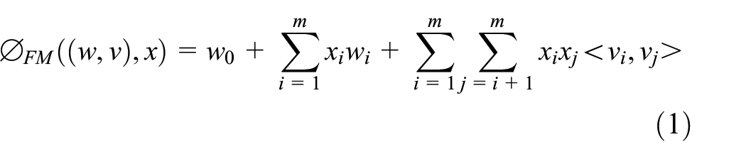
Ø_{FM} ((w, v), x) = w_{0} + \sum_{i = 1}^{m} x_{i} w_{i} + \sum_{i = 1}^{m} \sum_{j = i + 1}^{m} x_{i} x_{j} < v_{i}, v_{j} >

(1)

where w₀ is the global bias; w_i models the strength of the ith variable; x_i and x_j denote the ith and jth features, which are very sparse; and v_i and v_j are the embedding vectors corresponding to the features.

As we can see from equation (1), the equation can be generalized to unobserved cross parameters, making the FM model more robust. However, the FM model ignores the properties of features, such as different fields of features. Different fields of features may show different interaction behaviors.

FFM Models

FFM models such difference explicitly by learning n–1 embedding vectors for each feature, say i, and only using the corresponding one v_i,F_(j) to interact with another feature j from field F(j):

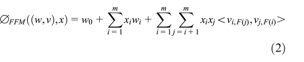
Ø_{FFM} ((w, v), x) = w_{0} + \sum_{i = 1}^{m} x_{i} w_{i} + \sum_{i = 1}^{m} \sum_{j = i + 1}^{m} x_{i} x_{j} < v_{i, F (j)}, v_{j, F (i)} >

(2)

where F(i) and F(j) are the field where features i and j are located, v_i and v_j represent the embedding vector when feature i interacts with feature j, and v_i,F_(j) represents feature i interacting with another feature j from field F(j).

The advantage of FFM is that it fully considers the differences in the interaction of features between different fields. The disadvantage is that the number of parameters is too high and it is too complicated, so it is not suitable for use in actual production.

FwFM Models

Like FFM, FwFM considers the difference in the interaction of features between different fields. The difference is that FwFM uses a scalar weight r to explicitly capture different interaction strengths of different field pairs. The core equation of the FwFM model is introduced as follows:

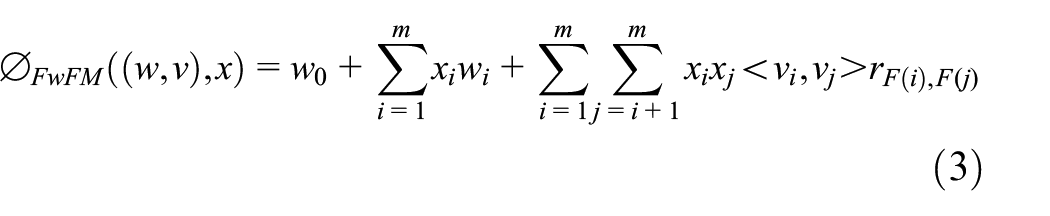
Ø_{FwFM} ((w, v), x) = w_{0} + \sum_{i = 1}^{m} x_{i} w_{i} + \sum_{i = 1}^{m} \sum_{j = i + 1}^{m} x_{i} x_{j} < v_{i}, v_{j} > r_{F (i), F (j)}

(3)

where v_i and v_j are the embedding vectors of feature i and feature j, F(i) and F(j) are the field to which feature i and feature j belong, and r is the weight of interaction strength of field F(i) and F(j).

The advantage of FwFM is to capture the interaction between different field features with only 4% of the parameters of FFM. The disadvantage is that only one scalar is used to express the strength of interaction between different fields, which has insufficient degrees of freedom and limited expression ability.

Deep Neural Network

DNN is an FNN, which includes an input layer, several hidden layers, and an output layer. Generally, the first layer is an input layer, which represents a low-dimensional dense vector. The last layer is called an output layer, which assigns a prediction score for each object. The middle layers between the input layer and the output layer are called hidden layers, which function as an automatic feature extractor. The DNN network takes the output of the previous layer as the input of current layer from the first hidden layer to the output layer. This process is called forward propagation. To make the calculated output fit the sample better, the method of back propagation is adopted to minimize the loss function. Forward propagation and back propagation are iterated many times until the stop criteria is reached.

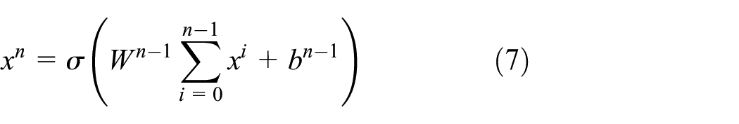
Equation (4) shows the calculation of the output of the kth layer x^k:

x^{k} = σ (W^{(k)} x^{k - 1} + b^{k})

(4)

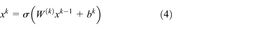
where σ represents the activation function, x^k–1 represents the output of the (k–1)th layer, and W^(k) and b^k are parameters of the kth layer.

DDNNFMFM Model

To meet the above requirements and follow the parallel structure of some mainstream frameworks, such as DeepFM, xDeepFM, DCN, and DeepLight, the DDNNFMFM model is proposed. The deep part of DDNNFMFM uses an improved DNN network, which can perform feature fusion with fewer parameters and improve the effect of implicit feature interaction. We name it the DenseDNN network; FmFM is selected for the shallow part, which uses a field matrix to simulate the explicit interaction between different field features, so as to further improve the accuracy of the model. DDNNFMFM combines deep model DenseDNN and shallow model FmFM in parallel, which can automatically learn implicit and explicit high-order feature interaction efficiently.

This section introduces the proposed neural network-based CTR prediction model, DDNNFMFM. The architecture of the DDNNFMFM model is shown in Figure 1. The model includes (a) an input layer, which represents each user-clicked advertisement data item with designed original features, yielding a high-dimensional sparse feature vector; (b) an embedding layer, which transforms the above high-dimensional sparse feature vector into a low-dimensional dense vector; (c) a deep learning DenseDNN model, which aims to extract effective implicit features from the low-dimensional vector; (d) a traditional FmFM model, which learns explainable explicit features from the low-dimensional vector; and (e) an output layer, which combines the deep implicit features obtained from DenseDNN and the shallow explicit features obtained from FmFM, and output and user-clicked prediction score. Each module will be introduced in the following sections.

Figure 1.

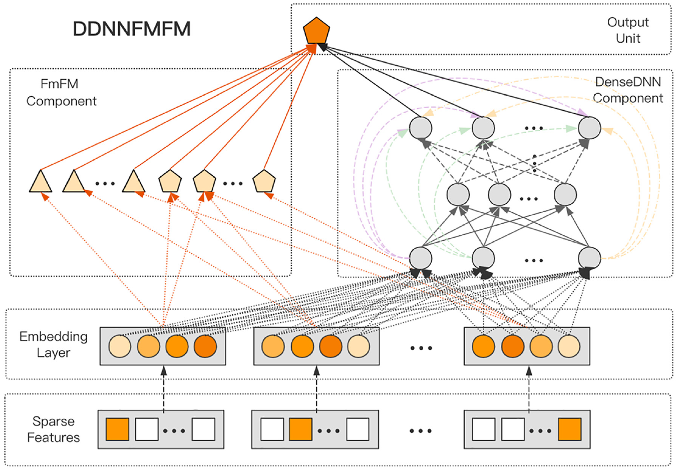
Structure of the DDNNFMFM model.

Input Layer

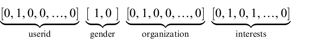
The input layer of the model represents a data item to a vector. In the field of advertising recommendation, the advertising data items clicked by users are usually very sparse, resulting in sparse and high-dimensional input features without temporal or spatial correlations. The original discrete features need to be one-hot encoded and converted into a one-hot vector x, where x is [ x₁, x₂, …, x_f ], and $x \in R^{d}$ , d is the dimension of the one-hot encoding vector, and f is the number of feature fields. Assuming that input data are sparse, the inputs are mostly categorical features [e.g. user_id = s02, gender = male, organization = MSRA, interests = comedy & Rock]. Such features are often encoded as high-dimensional sparse binary features. The aforementioned instance is illustrated as:

\underset{userid}{\underset{︸}{[0, 1, 0, 0, \dots, 0]}} \underset{gender}{\underset{︸}{[1, 0]}} \underset{organization}{\underset{︸}{[0, 1, 0, 0, \dots, 0]}} \underset{interests}{\underset{︸}{[0, 1, 0, 1, \dots, 0]}}

Embedding Layer

Nevertheless, the above one-hot encoding vectors often lead to high-dimensional spaces for large vocabularies; thus, we use an embedding layer to transform these binary features into dense vectors x to reduce the dimensionality (commonly called embedding vectors):

x_{embed, i} = W_{embed, i} x_{i}

(5)

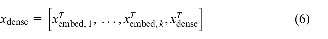
where x_i denotes the binary input in the ith category, x_embed,i denotes the embedding vector, and $W_{embed, i} \in R^{D \times K_{i}}$ is the corresponding embedding matrix.

Then, we stack multiple embedding vectors into one vector along with normalized dense features x_dense

x_{dense} = [x_{embed, 1}^{T}, \dots, x_{embed, k}^{T}, x_{dense}^{T}]

(6)

There are no combination features. We capture the interaction of a feature with a deep network and an FmFM model.

DenseDNN

Existing deep learning-based CTR prediction models can effectively capture high-order feature interactions and significantly improve the performance of the model. In recent years, the industry has proposed many CTR prediction models combined with DNNs in a parallel structure. Most of these parallel structure models improve the model performance by improving the shallow part of the model that studies explicit feature interactions. For example, the DeepFM model replaces the wide part of the Wide&Deep model with an FM model, the xDeepFM model designs a CIN network for shallow feature extraction, and the DeepLight model improves the FM model in DeepFM with an advanced FwFM model. However, the deep part usually uses DNNs in these parallel structure CTR prediction models, and there are few works focusing on improving the implicit feature interactions. To extract better implicit features, we can theoretically use more neural layers in the DNN network or use more neurons in each layer. However, practically, it will lead to problems such as gradient vanishing, gradient explosion, and excessive parameters, and the performance of DNN will decrease rapidly after reaching saturation with the increase of its layers.

To avoid the above problems, the DenseDNN network is proposed. DenseDNN introduces the idea of DenseNet to change the input of each layer of DNN into the sum of the outputs of all previous layers. Its model diagram is shown in Figure 2. Its advantages include: (a) alleviating the vanishing-gradient problem of deep network; (b) strengthening feature propagation; (c) substantially reducing the number of parameters; and (d) reducing the problem of sample over-fitting. Equation (7) is its output, where xⁱ represents the output of layer i, and W⁽ⁿ⁾ and bⁿ are training parameters.

x^{n} = σ (W^{n - 1} \sum_{i = 0}^{n - 1} x^{i} + b^{n - 1})

(7)

Figure 2.

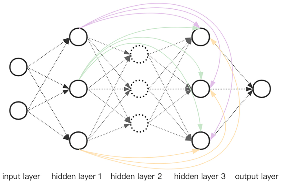
Structure of DenseDNN model.

FmFM models

The FmFM model is in line with the FM-based models, which also include the FM, FFM, and FwFM models. Similar to the FwFM model, we will learn an embedding vector for each feature. We define a matrix M_F_(i),F(j) to represent the interaction between field F(i) and field F(j) as follows:

x_{i} x_{j} < v_{i} M_{F (i), F (j)}, v_{j} >

(8)

where v_i, v_j are the embedding vectors of feature i and j, F(i) and F(j) are the fields of feature i and j, respectively, $M_{F (i), F (j)} \in R^{K \times K}$ is a matrix to model the interaction between field F(i) and field F(j). The complete formula of FmFM model is:

\begin{matrix} Ø_{FmFM} ((w, v), x) = w_{0} + \sum_{i = 1}^{m} x_{i} w_{i} \\ + \sum_{i = 1}^{m} \sum_{j = i + 1}^{m} x_{i} x_{j} < v_{i} M_{F (i), F (j)}, v_{j} > \end{matrix}

(9)

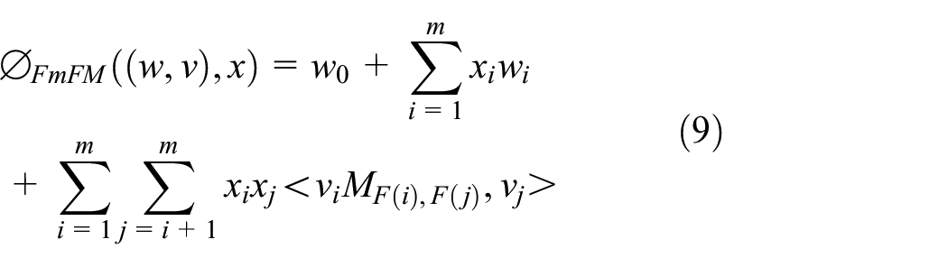
FmFM are extensions of FwFM in that it uses a two-dimensional matrix M_F_(i),F(j) to interact with different field pairs, instead of a scalar weight r in FwFM, which improves the degree of freedom and expression ability of the model. The interaction operation process is shown in Figure 3. The calculation of FmFM can be decomposed into three steps:

Embedding Lookup: the feature embedding vectors v_i, v_j, and v_k are looked up from the embedding table, and v_i will be shared between those two pairs.

Transformation: then v_i is multiplied by the matrices M_F_(i),F(j) and M_F_(i),F(k), respectively. Here we get the intermediate vector v_{i, F}_(j)=v_i×M_F_(i),F(j) for the field F(j), and v_i,F_(k)=v_i×M_F_(i),F(kj) for the field F(k).

Dot Product: the final interaction terms will be a simple dot product between v_j and v_{i, F}_(j), as well as v_k and v_{i, F}_(k), which are the black dots shown in Figure 3.

Figure 3.

An example of FmFM interaction term calculation.

Output Layer

After splicing the results of FmFM and DenseDNN, the output results are obtained through sigmoid function:

y = Sigmoid (y_{FmFM} + y_{DenseDNN})

(10)

where $y \in (0, 1)$ is the predicted CTR, y_FmFM is the output of FmFM component, and y_DenseDNN is the output of DenseDNN component.

Experiments

The experimental environment of this experiment is Windows 10 operating system, based on the Python 3.7.0, Tensorflow 2.3.0 framework. To verify the performance of the proposed model DDNNFMFM, a large number of comparative experiments were carried out on the two data sets of Criteo and Avazu to verify the performance of the model.

Experimental Setup

Data sets

Criteo Data set

This is a well-known benchmark data set for CTR prediction. This experiment uses Sample Criteo, which is the sampling of the Kaggle Criteo data set, with a total of 1 million samples. The first column represents whether the advertisement to be predicted is clicked. Each sample also has 13 columns of digital features, mainly counting features and 26 classification features. For the purpose of anonymity, these 26 classification features have been hashed to 32 bits.²⁵

Avazu Data set

This is used for Avazu CTR prediction competition, which predicts whether mobile advertising will be clicked. The Avazu data set has 40 million samples, and each sample has 23 classification fields. This article makes an experiment on 1 million data randomly sampled from Avazu data set.

Evaluation Metrics

Area Under the Curve

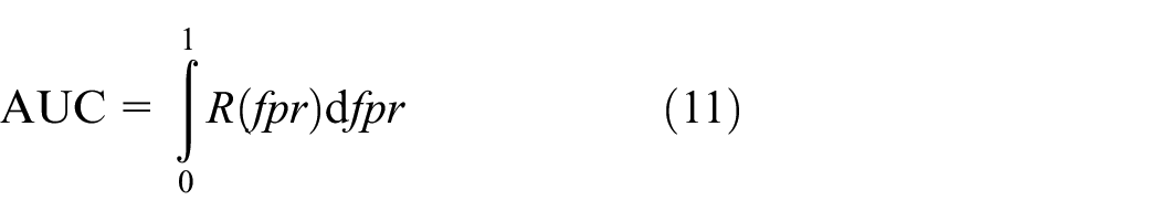
The Area Under the Curve (AUC) is the area under the ROC (Receiver Operating Characteristics) curve and takes a value between 0 and 1. The size of the AUC is positively correlated with the performance of the CTR prediction model. The calculation steps are as follows: (a) solve the values of true positive rate (TPR) and false positive rate (FPR) through the confusion matrix to obtain the coordinate point pair; (b) the curve formed by different coordinate point pairs is the ROC curve; (c) the AUC is the area below the ROC curve. The AUC is considered to be an important index of the CTR prediction problem, and its formula is:

AUC = \int_{0}^{1} R (fpr) d fpr

(11)

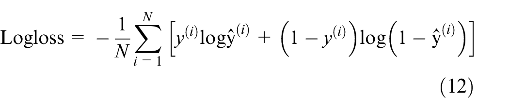
LogLoss

LogLoss is the binary cross-entropy loss function, which is used to evaluate the accuracy of the model and represent the distance between the predicted score and true label for each instance. Generally, we need to use the predicted probability to estimate the benefit of a ranking strategy. The formula is:

Logloss = - \frac{1}{N} \sum_{i = 1}^{N} [y^{(i)} \log {\hat{y}}^{(i)} + (1 - y^{(i)}) \log (1 - {\hat{y}}^{(i)})]

(12)

Data Processing

In the actual production activities, the data generated will be missing and abnormal. If directly used, it is easy to produce adverse results. Therefore, the missing part in the data set is filled in. To verify the performance of the model, the data set is divided into a training set, a verification set, and a test set according to the ratio of 8:1:1.

Model Comparison

In the individual model comparison experiment, LR, FM, CIN, and FwFM are selected as the models for learning explicit feature interaction to compare with FmFM used in DDNNFMFM, because FmFM is developed from LR, FM, and FwFM, and CIN is also used as a comparison model because it is a very classic and efficient model for learning high-order explicit feature interactions; the DNN model is compared with the DenseDNN proposed in this article, because DenseDNN is developed from the DNN model.

In the comprehensive model comparison experiment, shallow models LR, FM, FwFM, and FmFM are selected as the comparison models; the deep model DeepFM, xDeepFM, and DeepLight are selected as the comparison model, because they have similar architectures to DDNNFMFM and they are also the state-of-the-art models for CTR prediction.

Performance Evaluation

Individual Model

To verify the performance of DenseDNN and FwFM in DDNNFMFM, it can be seen from the comparison results of individual models in Table 1 that:

Learning feature interactions can improve the prediction results of the model. LR, as the only model without learning feature interaction, performs at least 1.1% on Criteo data set and 2.3% on Avazu data set worse than other methods in terms of the AUC, which shows that feature interactions are critical to improving the CTR prediction.

Compared with the individual model of explicit feature interaction, FmFM has the best performance on the Criteo data set and Avazu data set. It is proved that modeling the interaction of different field features as a matrix is conducive to the improvement of model performance.

Compared with DNN, the accuracy of DenseDNN proposed in this article improves by 0.29% on the Criteo data set and 0.70% on the Avazu data set in terms of the AUC, and reduces by 0.57% on the Criteo data set and 0.84% on the Avazu data set in terms of LogLoss, which proves that DNN has better performance after feature fusion.

Table 1.

Comparison of individual models on Criteo and Avazu data sets.

	Criteo		Avazu
	AUC	LogLoss	AUC	LogLoss
LR	0.7584	0.4737	0.7492	0.3943
FM	0.7768	0.4586	0.7664	0.3851
CIN	0.7836	0.4541	0.7737	0.3802
FwFM	0.7863	0.4499	0.7724	0.3814
FmFM	0.7880	0.4483	0.7756	0.3801
DNN	0.7817	0.4538	0.7693	0.3827
DenseDNN	0.7840	0.4512	0.7747	0.3795

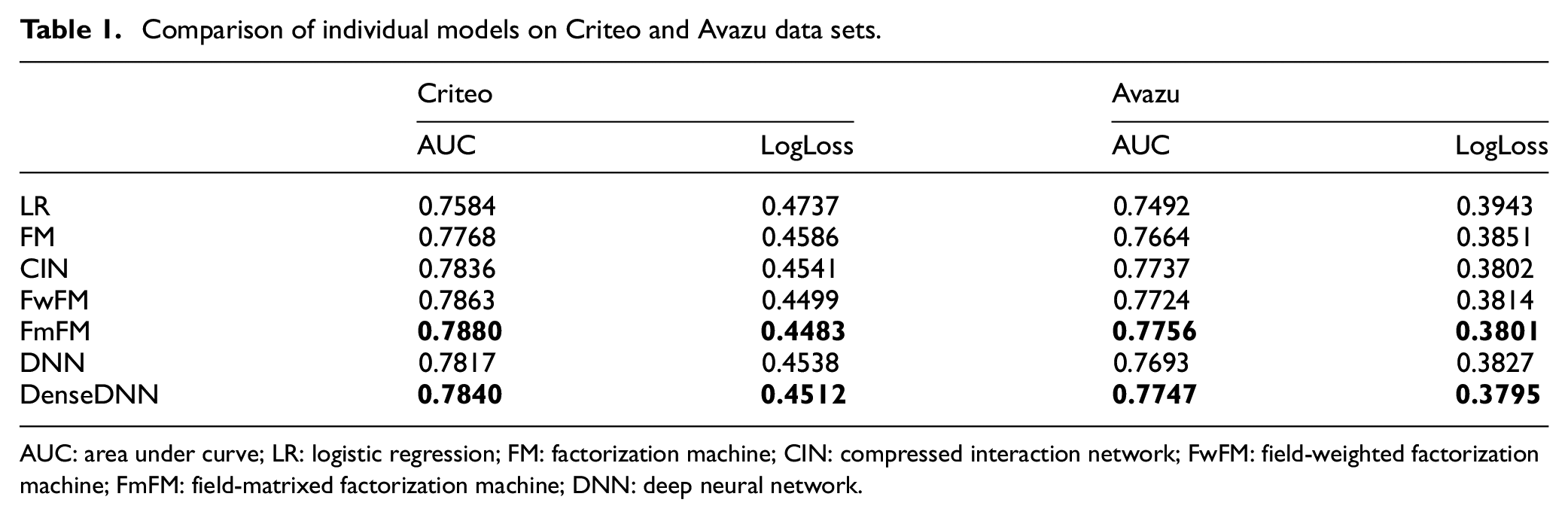
AUC: area under curve; LR: logistic regression; FM: factorization machine; CIN: compressed interaction network; FwFM: field-weighted factorization machine; FmFM: field-matrixed factorization machine; DNN: deep neural network.

Comprehensive Model

To verify the accuracy of DDNNFMFM, it can be seen from the comprehensive model comparison results in Table 2 that:

FmFM is not only a shallow model with the best performance, even in the Criteo data set, but also its performance is better than the classic deep learning models DeepFM and xDeepFM. This once again proves the advantage of the field matrix in the FmFM, which is lighter and faster than the two parallel models DeepFM and xDeepFM.

DDNNFMFM has the best effect among all models based on embedded neural network. As shown in Table 1, in the Criteo data set and the Avazu data set, compared with the classical suboptimal model DeepLight, the AUC of DDNNFMFM proposed in this article is increased by 0.21% and 0.41%, respectively, and the LogLoss is reduced by 0.36% and 0.35%, respectively.

Table 2.

Comparison of comprehensive models on Criteo and Avazu data sets.

	Criteo		Avazu
	AUC	LogLoss	AUC	LogLoss
LR	0.7584	0.4737	0.7492	0.3943
FM	0.7768	0.4586	0.7664	0.3851
FwFM	0.7863	0.4499	0.7724	0.3814
FmFM	0.7880	0.4483	0.7756	0.3801
DeepFM	0.7840	0.4526	0.7785	0.3772
xDeepFM	0.7869	0.4472	0.7793	0.3761
DeepLight	0.7940	0.4449	0.7890	0.3727
DDNNFMFM	0.7957	0.4433	0.7922	0.3714

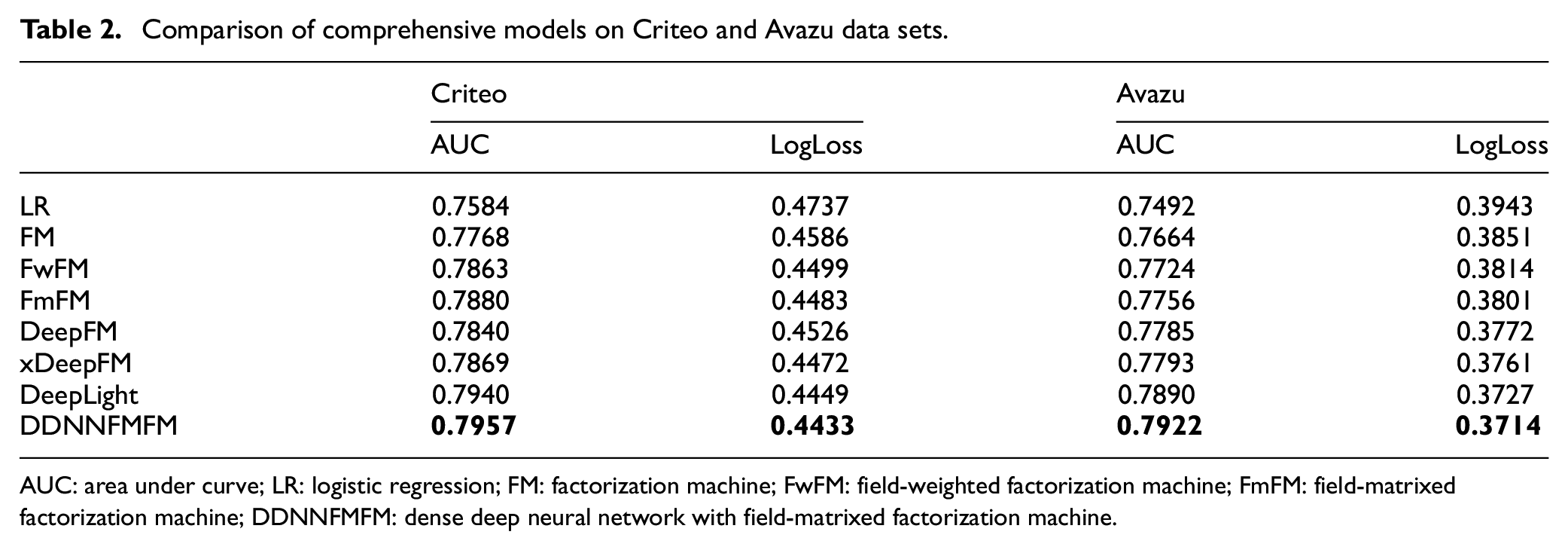
AUC: area under curve; LR: logistic regression; FM: factorization machine; FwFM: field-weighted factorization machine; FmFM: field-matrixed factorization machine; DDNNFMFM: dense deep neural network with field-matrixed factorization machine.

Hyper-Parameter Study

Number of Neurons Per Layer

Figure 4 shows the influence of the number of hidden layers in the Criteo data set on the experimental results. It can be seen that the DDNNFMFM model’s performance increases with the increase in network depth at the beginning, but when the network depth is greater than 5, the model performance declines, which is the result of over-fitting. The comparison models DeepFM, xDeepFM, and DeepLight perform best when the network depth is 3, because DDNNFMFM improves DNN, and feature fusion occurs only when the network depth is three layers and above. As a result, DDNNFMFM has the best result when the network depth of the hidden layer is 5.

Figure 4.

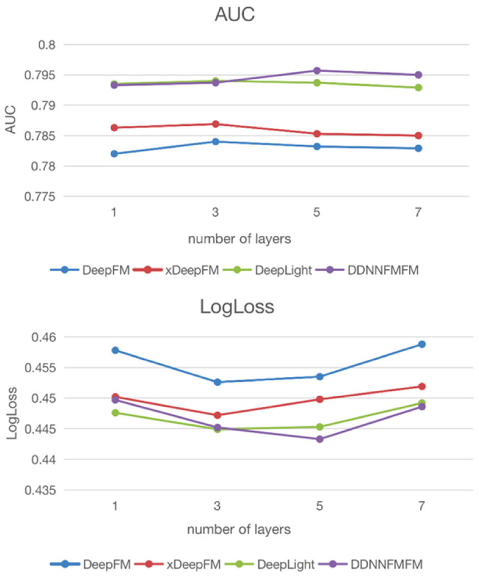
AUC and LogLoss comparison of number of layers.

Number of Hidden Layers

Figure 5 shows the influence of the number of neurons at each layer in the Criteo data set on the experimental results. In this comparative experiment, DDNNFMFM chooses the five layers with the best network depth. It can be seen that when the number of neurons is increased from 200 to 500, the performance of the model gradually improves and then declines, because the overly complex model is easy to overfit. The DDNNFMFM model performs best when the number of neurons is set to around 400.

Figure 5.

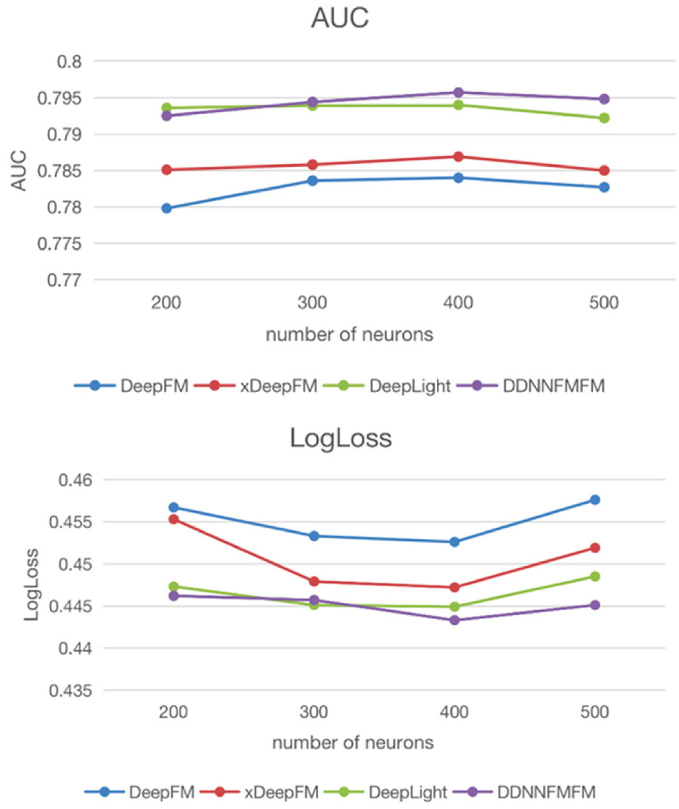
AUC and LogLoss comparison of number of neurons.

Conclusion

This article constructs a deep fusion network, DenseDNN, whose purpose is to deeply fuse features without deepening too many network layers or too many parameters to improve the performance of the model. To further improve the accuracy of CTR prediction model, following the parallel structure of some mainstream frameworks, the shallow model FmFM is combined with the deep model DenseDNN proposed in this article, and it is named DDNNFMFM. DDNNFMFM can automatically learn high-order feature interactions in both explicit and implicit ways, and carry out deep feature fusion while implicitly learning feature interactions, thus improving the accuracy of implicit learning feature interactions with a small cost. In this article, comprehensive comparative experiments are carried out on the Criteo data set and the Avazu data set to prove the effectiveness of DDNNFMFM. Compared with current mainstream deep learning-based models, such as DeepFM, xDeepFM, and DeepLight, DDNNFMFM has a great improvement in performance. In the practical application of advertising recommendation systems with huge data, a small increase in prediction accuracy may significantly increase the online CTR, which verifies the validity of DDNNFMFM in this article. In the future, further research will be done to reduce the complexity of DDNNFMFM by optimizing redundant parameters and network pruning, so as to better apply it to online advertising services.

Footnotes

Declaration of conflicting interests

The author(s) declared no potential conflicts of interest with respect to the research, authorship, and/or publication of this article.

Funding

The author(s) received no financial support for the research, authorship, and/or publication of this article.

ORCID iD

Yanxia Qin

References

Chen

, et al. Attentive capsule network for click-through rate and conversion rate prediction in online advertising. Knowl Based Syst 2021; 211: 106522.

Zhang

Yan

Zhang

CTR prediction models considering the dynamics of user interest. IEEE Access 2020; 8: 72847–72858.

Deng

Liu

Research on click-through rate prediction of advertisement based on GMM-FMs. Comput Eng 2019; 45(5): 122–126.

Chapelle

Manavoglu

Rosales

Simple and scalable response prediction for display advertising. ACM Trans Intell Syst Technol 2015; 5(4): 1–34.

Liu

Zeng

Yue

, et al. A hybrid network based CTR prediction model for online advertising. Chin J Comput 2019; 42(7): 1570–1587.

Wen

Yuan

Qin

, et al. Neural attention model for recommendation based on factorization machines. Appl Intell 2021; 51(4): 1829–1844.

Juan

Y-C

Zhuang

Chin

W-S

, et al. Field-aware factorization machines for CTR prediction. In: RecSys ’ 2016, 2016, pp. 43–50, https://www.csie.ntu.edu.tw/∼cjlin/papers/ffm.pdf

Pan

Ruiz

, et al. Field-weighted factorization machines for click-through rate prediction in display advertising. In: WWW ’18: Proceedings of the web conference, 2018, pp. 1349–1357, https://dl.acm.org/doi/fullHtml/10.1145/3178876.3186040

Sun

Pan

Zhang

, et al. FM2: Field-matrixed factorization machines for recommender systems. In: WWW ’21: Proceedings of the web conference, 2021, pp. 2828–2837, https://dl.acm.org/doi/10.1145/3442381.3449930

10.

Zhang

Wang

. Deep learning over multi-field categorical data: A case study on user response prediction. In: ECIR 2016: Advances in information retrieval, 2016, pp. 45–57, https://link.springer.com/chapter/10.1007/978-3-319-30671-1_4

11.

Cai

Ren

, et al. Product-based neural networks for user response prediction. In: 2016 IEEE 16th international conference on data mining (ICDM), 2016, pp. 1149–1154, https://ieeexplore.ieee.org/document/7837964

12.

Heng-Tze

Levent

Jeremiah

, et al. Wide & deep learning for recommender systems. In: DLRS 2016: Proceedings of the 1st workshop on deep learning for recommender systems, 2016, pp. 7–10, https://dl.acm.org/doi/10.1145/2988450.2988454

13.

Guo

Tang

, et al. DeepFM: A factorization-machine based neural network for CTR prediction. In: Proceedings of the 26th international joint conference on artificial intelligence (IJCAI-17), 2017, pp. 1725–1731, https://www.ijcai.org/proceedings/2017/0239.pdf

14.

. An efficient intrusion detection model based on deepFM. In: 2020 IEEE 4th information technology, networking, electronic and automation control conference (ITNEC), 2020, pp. 778–783, https://ieeexplore.ieee.org/document/9084722

15.

Wang

, et al. Deep & cross network for ad click predictions. In: Proceedings of the ADKDD’ 17, 2017, pp. 1–7, https://dl.acm.org/doi/10.1145/3124749.3124754

16.

Lian

Zhou

Zhang

, et al. xDeepFM: Combining explicit and implicit feature interactions for recommender systems. In: KDD ’18: Proceedings of the 24th ACM SIGKDD international conference on knowledge discovery & data mining, 2018, pp. 1754–1763, https://dl.acm.org/doi/10.1145/3219819.3220023

17.

Wang

Shivanna

Cheng

, et al. DCN V2: Improved deep & cross network and practical lessons for web-scale learning to rank systems. In: WWW ’21: Proceedings of the web conference 2021, 2021, pp. 1785–1797, https://dl.acm.org/doi/10.1145/3442381.3450078

18.

Deng

Pan

Zhou

, et al. DeepLight: Deep lightweight feature interactions for accelerating CTR predictions in ad serving. In: WSDM ‘21: Proceedings of the 14th ACM international conference on web search and data mining, 2021, pp. 922–930, https://dl.acm.org/doi/10.1145/3437963.3441727

19.

Duan

Zheng

, et al. A CTR prediction model based on user interest via attention mechanism. Appl Intell 2020; 50(4): 1192–1203.

20.

Zhang

Wang

. Deep interaction network based CTR prediction model. In: 2020 13th international symposium on computational intelligence and design (ISCID), 2020, pp. 286–289, https://ieeexplore.ieee.org/document/9325800

21.

Xiao

, et al. Attentional factorization machines: Learning the weight of feature interactions via attention networks. In: Proceedings of the 26th international joint conference on artificial intelligence (IJCAI-17), 2017, pp. 3119–3125, https://www.ijcai.org/proceedings/2017/0435.pdf

22.

Huang

Zhang

. FiBiNET: Combining feature importance and bilinear feature interaction for click-through rate prediction. In: RecSys ‘19: Proceedings of the 13th ACM conference on recommender systems, 2019, pp. 169–177, https://dl.acm.org/doi/10.1145/3298689.3347043

23.

Song

Shi

Xiao

, et al. AutoInt: Automatic feature interaction learning via self-attentive neural networks. In: CIKM ’ 19, 2019, pp. 1161–1170, https://arxiv.org/pdf/1810.11921.pdf

24.

Cheng

Chen

, et al. Interpretable click-through rate prediction through hierarchical attention. In: WSDM ‘20: Proceedings of the 13th international conference on web search and data mining, 2020, pp. 313–321, https://dl.acm.org/doi/10.1145/3336191.3371785

25.

Criteo Labs. Display advertising challenge, 2014, https://www.kaggle.com/c/criteo-display-ad-challenge

A Novel Click-Through Rate Prediction Model Based on Deep Feature Fusion Network

Abstract

Keywords

Introduction

Related Work

Shallow Feature Extraction Models

FM Models

FFM Models

FwFM Models

Deep Neural Network

DDNNFMFM Model

Input Layer

Embedding Layer

DenseDNN

FmFM models

Output Layer

Experiments

Experimental Setup

Data sets

Criteo Data set

Avazu Data set

Evaluation Metrics

Area Under the Curve

LogLoss

Data Processing

Model Comparison

Performance Evaluation

Individual Model

Comprehensive Model

Hyper-Parameter Study

Number of Neurons Per Layer

Number of Hidden Layers

Conclusion

Footnotes

Declaration of conflicting interests

Funding

ORCID iD

References