Sage Journals: Discover world-class research

Abstract

This paper presents deep learning neural network models for photovoltaic output current prediction. The proposed models are long short-term memory and gated recurrent unit neural networks. The proposed models can predict photovoltaic output current for each second for a week time by using global solar radiation and ambient temperature values as inputs. These models can predict the output current of the photovoltaic system for the upcoming seven days after being trained by half-day data only. Python environment is used to develop the proposed models, and experimental data of a 1.4 kWp PV system are used to train, validate and test the proposed models. Highly uncertain data with steps in seconds are used in this research. Results show that the proposed models can accurately predict photovoltaic output current whereas the average values of the root mean square error of the predicted values by the proposed LSTM and GRU are 0.28 A and 0.27 A (the maximum current of the system is 7.91 A). In addition, results show that GRU is slightly more accurate than LSTM for this purpose and utilises less processor capacity. Finally, a comparison with other similar methods is conducted so as to show the significance of the proposed models.

Keywords

Photovoltaic prediction deep learning machine neural network

Introduction

Recently, photovoltaic (PV) energy is attracting focus as it is clean, abundant and environment friendly. PV systems can be grid connected system, standalone PV systems and hybrid PV systems. With all types of the aforementioned systems, accurate control of system's performance is required depending on system's types and configuration (Khatib and Elmenreich, 2016). As a fact, in all control techniques, PV system output power or current is a control key factor whereas the whole control strategy is done based on that (Bermejo et al., 2019). PV output current is usually preferred in all types of control system, as it is the varying factor while system's voltage is usually maintained by using power electronic features (Yang et al., 2014). PV output current varies according to solar radiation and ambient temperature. The relation between PV output current and solar radiation is proportional and is considered the most important relation as compared to the relation of PV output current with another factors such as solar cell temperature (Yang et al., 2014). Thus, due to the nature of the global solar radiation (sun rays inside the atmosphere), the uncertainty of PV systems’ output current is a major challenge for any prediction model (Yang et al., 2014). The uncertainty of PV output current is usually because of the uncertainty of the global solar radiation which is because of clouds movement and other weather conditions.

Based on that, many researchers have proposed models to predict the output current (sometimes output power) of the PV system. These models can be classified as empirical models, statistical models and artificial neural network based models (Ayompe et al., 2010). Here the prediction of PV system output power and output current does not matter and are considered similar as system's voltage is considered stable during operation time.

In (Ayompe et al., 2010) PV system output power prediction is done empirically by proposing models for PV modules cell temperature and efficiency. The idea in such a model is to predict the output power depending on the ideal theoretical value, and then by estimating system's losses and efficiency, the final value of the output power is predicted. Similar examples of empirical models are presented in (Cucumo et al., 2006; Durisch et al., 2007; Hove, 2000; Navabi et al., 2015; Wang et al., 2015). Empirical models are considered accurate under stable solar radiation conditions. However, under highly uncertain solar radiation condition, these models fall to predict the output power of the system in an accurate way.

On the other hand, PV output power or current can be predicted by time series and regression models (Bacher et al., 2009; Hammer et al., 1999; Li et al., 2014; Ran and Guangmin, 2008). These models can predict PV output power accurately in a well-behaved PV system with stable performance (Wong et al., 2010). However, here also such models fall to perform well under highly uncertain conditions.

Thus, artificial neural networks (ANNs) models as alternative models are proposed to overcome the drawbacks of empirical and statistical models. Artificial neural network based models are used to overcome the problem of the uncertain weather conditions that is usually represented by a non-linear relationship between the input vector and the output vector (target). The self-learning ability of ANNs is the key feature that helps in overcoming the impact of uncertain weather conditions. Thus, the proposal of ANNs shows accurate models that are able to predict PV output power or current under all weather conditions. In (Sulaiman et al., 2012), hybrid multi-layer feed forward neural network is used to prediction the output power of PV system. The proposed model used solar radiation and PV module's temperature as input variables. However, a very short dataset was used in this research for training and testing. This actually limited the proposed model from being expert in all year weather profile and consequently affected its ability to predict future targets. Meanwhile, in (Brano et al., 2014) different topologies of ANNs are proposed for PV output power perdition. Three types of ANNs were utilised in this research which were multilayer layer perceptron (MLP), gamma memory (GM) trained with the back propagation and a recursive neural network (RNN). The proposed models were trained using ambient temperature, solar radiation and wind speed. Meanwhile, historical PV output power dataset was used as a target. After that, a comparison between the proposed models was done so as to pick out the best model based on prediction accuracy. More examples of ANNs based models for PV system output power prediction can be found in (Ameen et al., 2015; Chow et al., 2012).

In all previous ANN based models (Ameen et al., 2015; Brano et al., 2014; Chow et al., 2012; Sulaiman et al., 2012), the prediction process is accurate in a very good way, however, models accuracy is not everything to consider when comparing these models. In most of these models (Ameen et al., 2015; Brano et al., 2014; Chow et al., 2012; Sulaiman et al., 2012), the authors have used large dataset (at least for one year time) to train the models. These datasets were mostly hourly datasets but in sometimes these datasets were in seconds such as in (Ameen et al., 2015). This means that these datasets are huge to handle and process. However, the use of such huge datasets is a must so as to allow the models to master the nonlinear relation between input vector and output vector under highly uncertain weather conditions. Here as far as the dataset is large, the required computational power becomes higher and the way to embed these models becomes harder. In fact, no one has discussed this issue before as most of these researchers are conducted by using normal computers or super computers where such a problem will never pop up. However, when it comes to ANNs based models that are applied to physical systems such as PV systems or electrical power systems, the easiness of embedding this model is one of the most important issues to be considered. Thus, there is a dire need to have ANNs based models that can be trained by using minimum data and have the ability then to predict future data in accurate way. It is also important to have models that are able to handle the uncertainty of weather conditions. All these features should be in the desired model at minimum computational power and processing time.

For this purpose deep learning based ANNs were proposed before for such a purpose such as long short-term memory (LSTM) and gated recurrent unit (GRU) neural networks (Zang et al., 2020) The authors of (Zang et al., 2020) has stated that deep learning machines such as LSTM and GRU are better than artificial neural network and scalar vector machine based models for solar radiation prediction especially in short-term form. In (Lee and Kim, 2019), the authors utilised LSTM to predict one day a head of solar radiation by using a 30 min step dataset. The authors have used solar radiation as an input. This means that the prediction was an online ahead prediction. The average root mean square error for this process was about 8.2 W/m². Similar work was done in (Ghimire et al., 2019) but by using hourly dataset. GRU was also utilised in (Ghimire et al., 2019) beside LSTM. This research showed the importance of using dataset with small step whereas the use of hourly dataset makes the RMSE for the LSTM model reaches 109 W/m², while it was 59 W/m² for GRU. By comparing these results to the results of (Lee and Kim, 2019), it is very clear that the step of the dataset plays an important role in obtaining accurate results. In (Aslam et al., 2019) the authors predicted a one day ahead of solar radiation by using LSTM based on hourly step dataset as well, but with an input vector that contains temperature, humidity, wind speed, visibility and dew point. The increase of inputs increases the accuracy of LSTM model to be 76 W/m² as compared to (Ghimire et al., 2019). Based on that, many researchers have considered more inputs to increase the accuracy of the LSTM model as in (He et al., 2020; Jeon and Kim, 2020; Qing and Niu, 2018; Wojtkiewicz et al., 2019). In (Yu et al., 2019), the authors have used a one minute step database to train LSTM and GRU models for solar radiation prediction of 30 min ahead. The RMSE values were 58 W/m² and 55 W/m² respectively.

Similar methodologies were presented to model PV output power based on LSTM and GRU models (Abdel-Nasser and Mahmoud, 2019; Lee et al., 2019; Lee and Kim, 2019; Li et al., 2019; Wang et al., 2018, 2019; Wen et al., 2019; Yan et al., 2020). In all of these methods input vectors that contain ambient temperature, wind speed, humidity, solar radiation, wind direction, direct solar radiation and diffuse solar radiation were used for online prediction. In some other cases only PV power was used for short term prediction (online a head prediction). All of these methods which are presented in (Abdel-Nasser and Mahmoud, 2019; Lee et al., 2019; Lee and Kim, 2019; Li et al., 2019; Wang et al., 2018, 2019; Wen et al., 2019; Yan et al., 2020) are based on hourly datasets, while a maximum of “one day ahead” prediction was done in these researches. Thus, in this research it is aimed to propose LSTM and GRU models for longer term prediction as compared to the methods in (Abdel-Nasser and Mahmoud, 2019; Lee et al., 2019; Lee and Kim, 2019; Li et al., 2019; Wang et al., 2018, 2019; Wen et al., 2019; Yan et al., 2020). The significance of this research as compared to other researches, that it aims to propose a model to predict a one week ahead (seven days) based on minimum training data (half-day) by using very sensitive dataset (second step data). This assures proposing an accurate model that is capable of predicting one week time of PV power records under uncertain conditions at minimum requirements of computational power and training data.

Photovoltaic output current characteristics and models

Figure 1 shows the one diode model equivalent circuit for a solar cell output. The equivalent circuit consists of a current source that represents the photo current of the solar cell, a reverse diode which represents the solar cell in the absence of sunlight, a shunt resistance which has a very large value and it represents the surface quality along the periphery and a series resistance with a very small value that represents the contact resistance between the semiconductor and the metal. The value of the shunt resistance is very large compared to the series resistance. and therefore it can be neglected.

Figure 1.

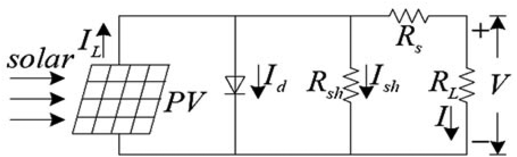
Pv module equivalent circuit.

From Figure 1, the solar cell output current (I_L) is given by the following relation (Khatib and Elmenreich, 2016);

I_{L} = I_{p h} - I_{d} - I_{R s h}

(1)

where (

I_{p h}

) represents the photocurrent, I_d represents the diode current and I_Rsh is the shunt resistance current. The diode current can be also given by,

I_{d} = I_{0} [\exp \frac{q (V_{p v} + I_{p v} R_{S})}{n k T} - 1]

(2)

while,

I_{R s h} = \frac{V_{p v} + I_{p v} R_{S}}{R_{s h}}

(3)

By combining equation (1)–(3),

I_{L}

can be given by (Khatib and Elmenreich, 2016);

I_{L} = I_{p h} - I_{0} [\exp \frac{q (V_{p v} + I_{p v} R_{S})}{n k T} - 1] - \frac{V_{p v} + I_{p v} R_{S}}{R_{s h}}

(4)

where k is the Boltzmann's constant, q is the electric charge of an electron, T is cell temperature and n is the ideality factor of the diode. Meanwhile, the solar cell output current, I_L is a function of T₁ and T₂ which are the temperatures at reference testing conditions, and can be calculated by (Khatib and Elmenreich, 2016);

I_{L} = I_{L} (T_{1}) + K_{0} (T - T_{1})

(5)

where

I_{L} (T 1) = I_{s c T 1, n o m} [\frac{G}{G_{n o m}}]

(6)

K_{0} = \frac{I_{s c T} - I_{s c T 1}}{T_{2} - T_{1}}

(7)

where G is the irradiance and

G_{n o m}

is the irradiance at the reference test

The diode saturation current, $I_{0}$ can be calculated by,

I_{0} = I_{0 T 1} {(\frac{T}{T_{1}})}^{3 / n} \exp^{\frac{q v_{q T_{1}}}{n k ((1 / T) - (1 / T 1))}}

(8)

where

I_{0 T 1} = \frac{I_{S C T 1}}{(\exp \frac{q V_{o c} T 1}{n k T 1} - 1)}

(9)

Meanwhile, the series resistance of a PV module is given by (Khatib and Elmenreich, 2016);

R_{s} = - \frac{d V}{d I V_{o c}} - \frac{1}{X_{V}}

(10)

where

X_{V} = I_{0 T 1} \frac{q}{n k T 1} \exp \frac{q V_{o c} T 1}{n k T 1}

(11)

As a fact, metrological data affect the performance of the PV system. Changing solar radiation and ambient temperature affect the output current and voltage produced by a PV module proportionally. Increasing solar radiation increases the output current of a PV module in a linear pattern and PV module's voltage in a logarithmic pattern. On the other hand, the increase of ambient temperature reduces the PV modules output voltage linearly and the PV module output current logarithmically.

A typical grid connected PV system (GCPV) is usually consisted of a PV array and power conditioners such as maximum power point tracker and inverter. The general working concept of GCPV is that the incident radiation of the sun on the PV array is collected and converted to a DC current. This DC current is injected to the grid after passing through a controller and an inverter. Thus, the output current of a PV array can be described as follows (Khatib and Elmenreich, 2016).

I_{P V} (t) = \frac{[P_{m} (G_{T} (t) / G_{r n o r m}) - α_{T} (T_{c} (t) - T_{r e f e r e n c e})]}{V_{P V} (t)}

(12)

where G_T is the collected solar radiation in (W/m²), G_norm is the solar radiation at reference conditions in (W/m²), V_PV is PV array voltage, α_T is the temperature coefficient of the PV module power which is given by the manufacturer, T_reference is the ambient temperature at reference conditions, η_inv and η_wire are the efficiencies of the inverter and the wires, respectively. T_c is the solar cell temperature and it can be calculated by the following equation:

T_{c} (t) = T_{a m b} (t) + ((\frac{N O C T - 20}{800}) \times G_{T} (t))

(13)

where T_amb is the ambient air temperature in °C and NOCT is the normal operating cell temperature in °C. NOCT represents the cell temperature of a PV module when ambient temperature is 20°C, solar radiation is 800 W/m² and wind speed is 1 m/s (Khatib and Elmenreich, 2016).

Regression analysis can be considered as one of the most famous techniques that are used for analysing multi factor data. Regression analysis is a statistical process that is utilised to predict and express the relationships between the variables of interest (dependent variable and independent variables). The simplest regression model is represented by a simple linear regression model which is a model with a single explanatory variable that has a relationship with the response in straight line as illustrated below (Khatib and Elmenreich, 2016),

I_{P V} (t) = β_{o} + β_{1} G_{T} (t)

(14)

where β_o the intercept, and β₁ is the slope of the line.

On the other hand, other form of regression analysis is the multiple regression models. This model considers more than one independent variable. In other words, multiple regressions simultaneously consider the influence of multiple explanatory variables on a response variable. The basic model for linear multiple regression is (Khatib and Elmenreich, 2016),

I_{P V} (t) = β_{o} + β_{2} G_{T} (t) + β_{3} T_{a m b} (t)

(15)

where β_o the intercept and (β₂, β₃) are the regression coefficients.

Proposed deep learning machines models

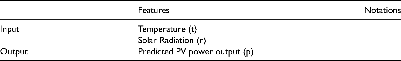
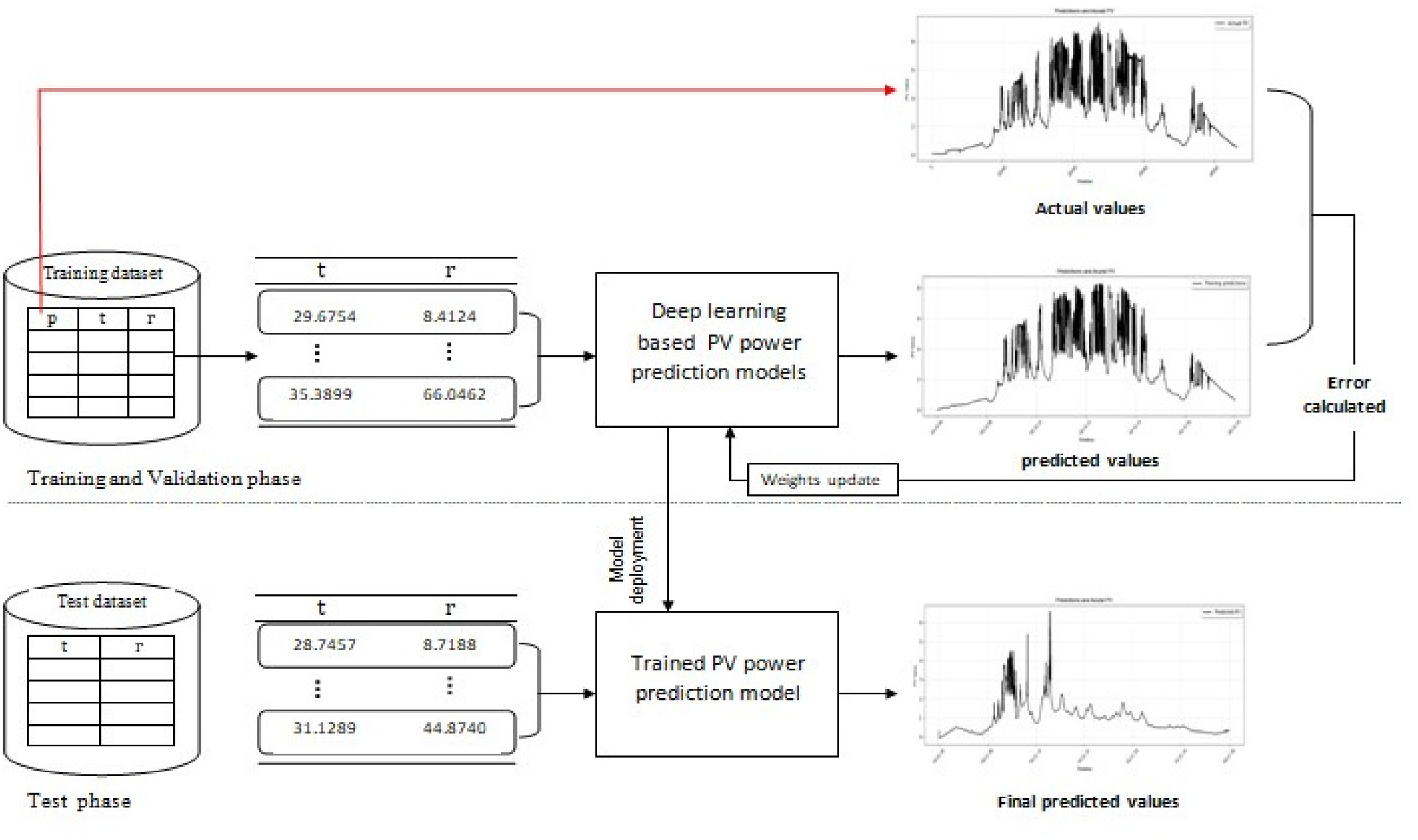
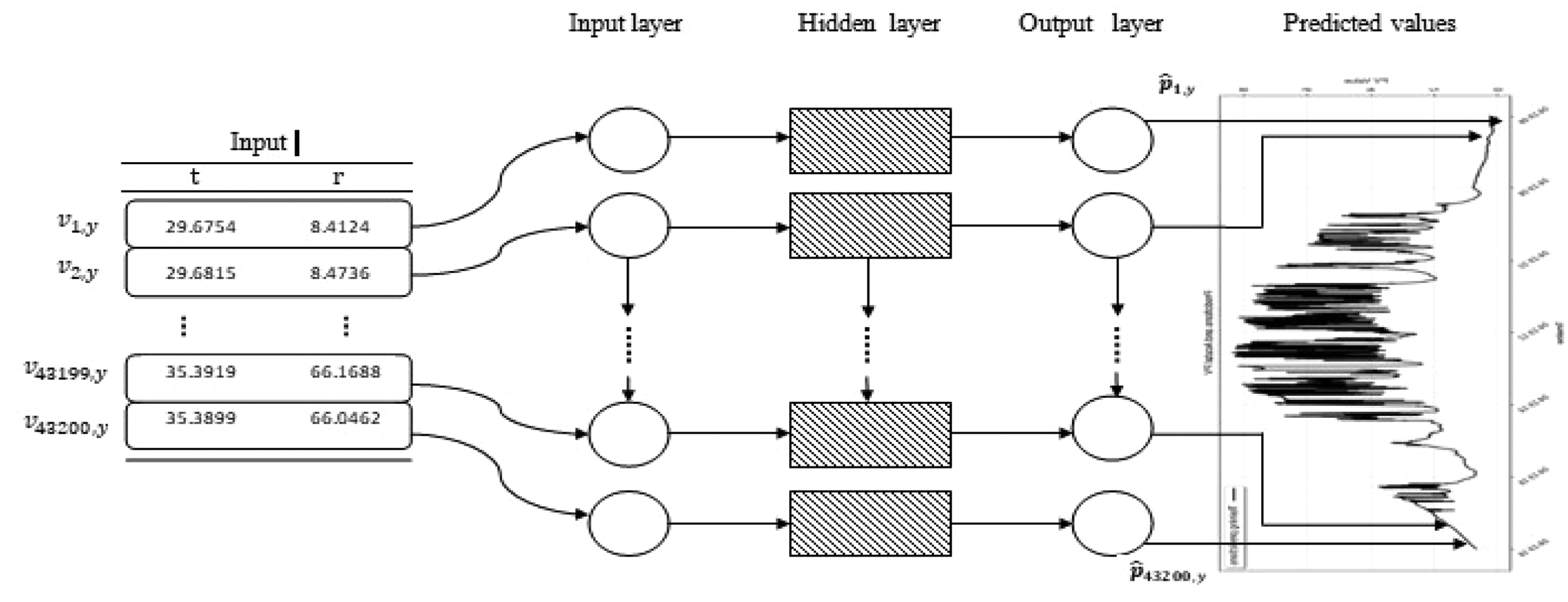
In this paper, two deep learning based machines are proposed to predict the output current of a photovoltaic system with high sensitivity. The predicted values are in seconds and based on two main meteorological factors which are ambient temperature and solar radiation. Long short-term memory (LSTM) artificial recurrent neural network and Gated recurrent unit (GRU) neural network are used for this purpose. The data utilised in this research are data for seconds with high variation of daylight so as to reflect the uncertainty in system's output. Table 1 shows the utilised inputs and outputs for the proposed model.

Table 1.

Notations of the inputs and output for the x-th second in the j-th day utilised in the proposed models.

	Features	Notations
Input	Temperature (t)	$t_{x, y}$
Input	Solar Radiation (r)	$r_{x, y}$
Output	Predicted PV power output (p)	${\hat{p}}_{x, y}$

For representing the status of the x-th second in the y-th day, a two dimensional input vector, are assumed as below,

v_{x, y} =< t_{x, y}, r_{x, y} >, x = 1, \dots, n, y = 1, \dots m .

(16)

where n means the number of seconds to predict, and m is the number of days.

The utilised data are divided into two sets which are training and testing sets. The training set is a set of n input vectors that consists of ambient temperature records and solar radiation records for the y-th day. Meanwhile, the training samples are entered respectively to avoid using the x-th second and y-th day as inputs which means fewer inputs as shown in Figure 2.

Figure 2.

Proposed neural network framework for secondly PV power prediction.

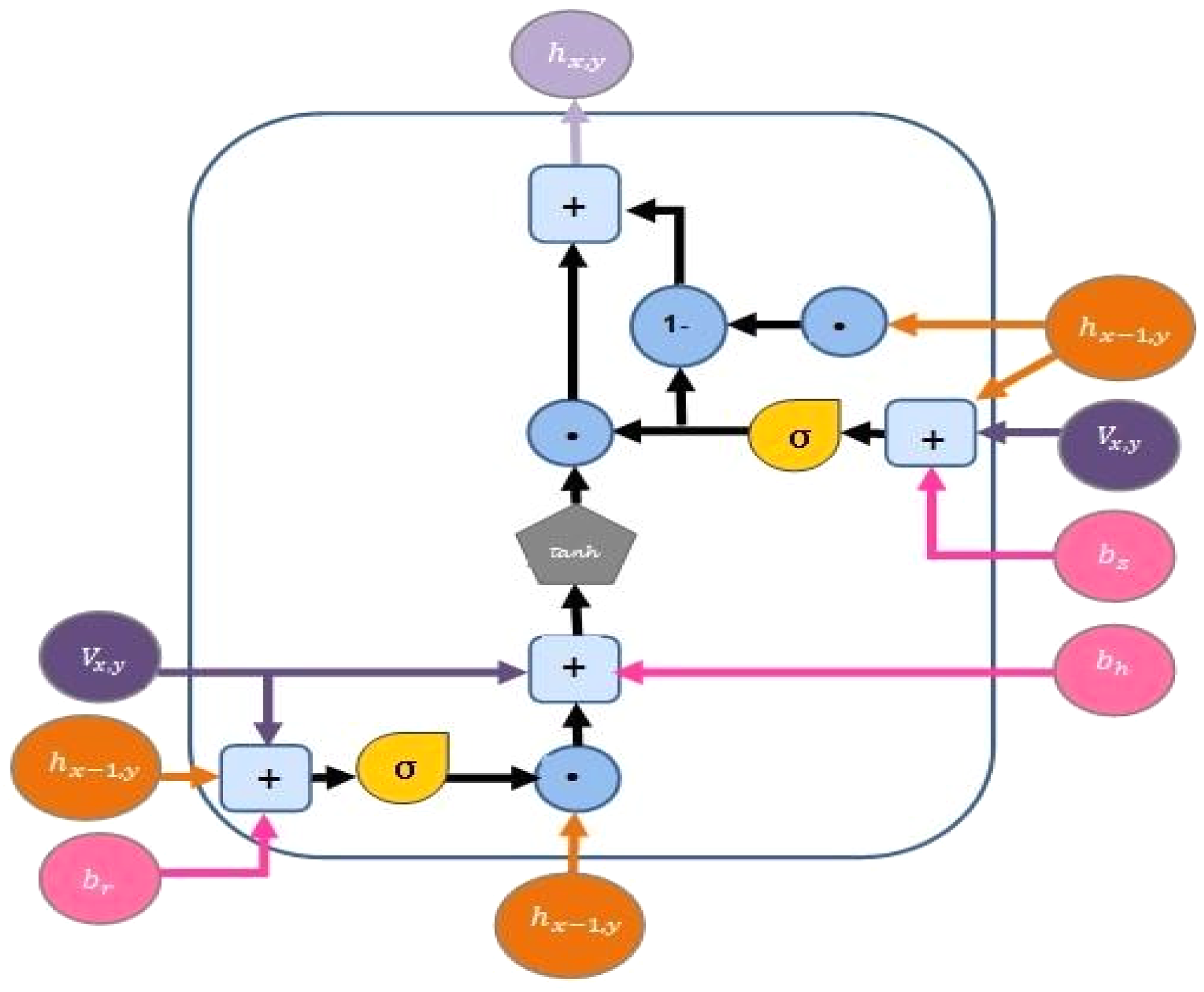
The proposed model consists of an input layer with n nodes, where each node is for a particular second, and an output layer with n nodes, where each node is for a particular second corresponding to its input node. Data for one solar day in seconds is only used in the training (6:00am–6:00pm) for the y-th day. These data are represented by 43,200 nodes in the training process as illustrated in Figure 3.

Figure 3.

Structure of the proposed GRU model for secondly PV output current prediction.

LSTM-Based PV output current prediction

LSTM-based model is developed in a way to capture the sequential PV power output patterns hidden across days. In other words, LSTM model tries to learn the long-term relationships among ambient temperature and solar radiation. In addition, it understands the short-term relationships across the PV output power records. The proposed model consists of a block that is called a block cell. This cell collectively determines the intermediate outputs based on the current and the past input values by utilising the long- and short-term sequential memories, which is the basic concept of LSTM (Sharadga et al., 2020). Figure 4 illustrated the main concept of the utilised LSTM model.

Figure 4.

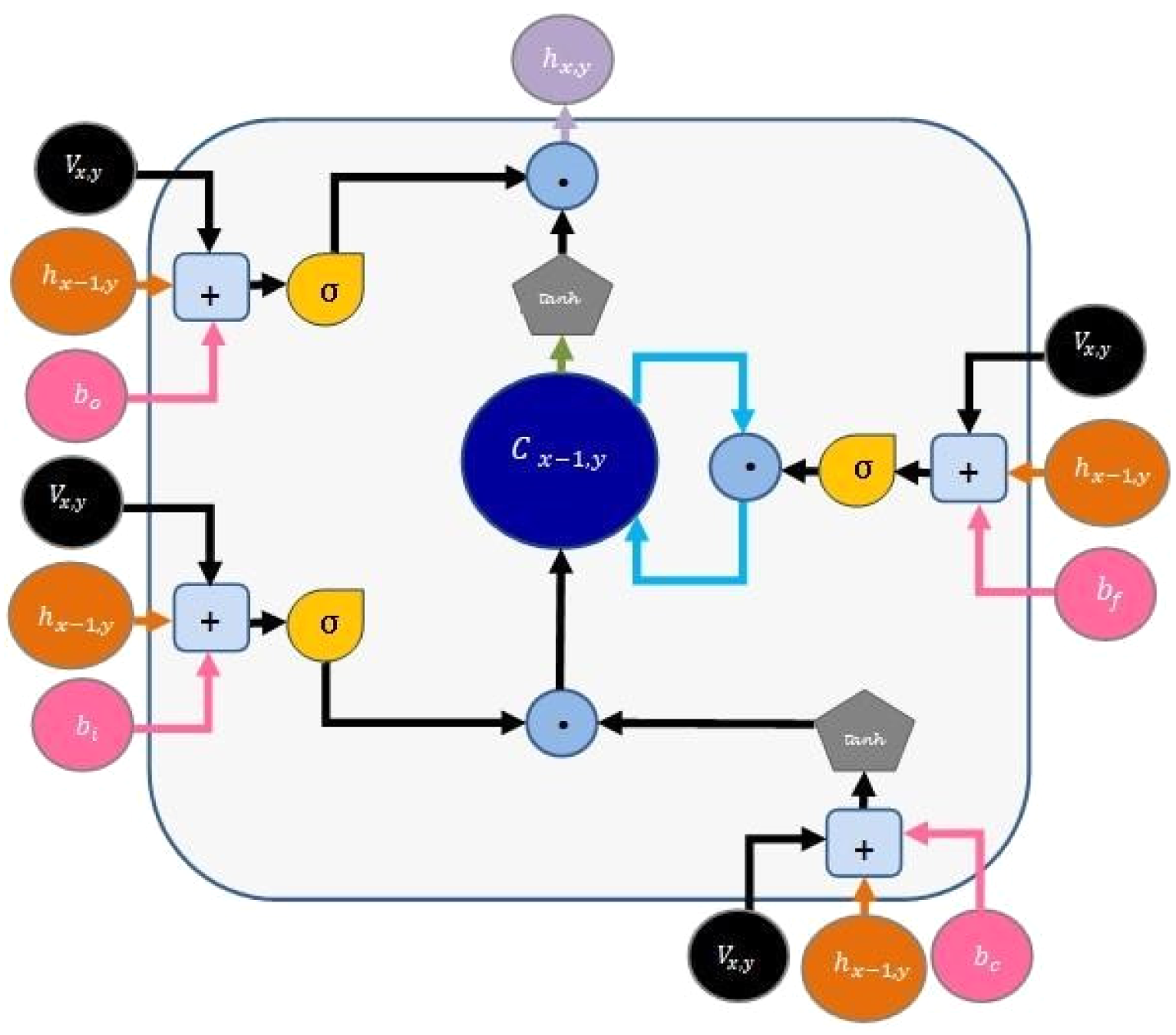
Block cell structure of the proposed LSTM model.

From Figure 4, the construction of a block cell for the x-th second in the y-th day consists of three gates: input, forget and output gates denoted as $i_{x, y}$ , $f_{x, y}$ and $o_{x, y}$ , respectively. Here, $h_{x, y}$ means the output of the current cell. In addition, $b_{i}$ , b_i and b_f are the bias vectors. $c_{x, y}$ is the cell state for the current block and ${\tilde{c}}_{x, y}$ is the candidate value for the cell state. $w_{h_{i}}$ , $w_{h_{f}}$ and $w_{h_{o}}$ are the weight matrices for the input, forget and output gates respectively.

Sigmoid function is applied in this research for the weighted summations of the inputs. The past outputs and the bias values for each gate to calculate the output for each of the three gates accordingly as three main steps.

The output for the update gate is calculated using equation (17).

i_{x, y} = σ (w_{v_{x, y} i} v_{x, y} + w_{h_{i}} h_{x - 1, y} + b_{i})

(17)

This value indicates how much of the candidate value are used for the current cell. The values of both forget and update gates varies between 0 and 1.

Meanwhile, the output for the forget gate is calculated using equation (18). This value indicates how much information is obtained from the previous cell which is used for the current cell.

f_{x, y} = σ (w_{v_{x, y} f} v_{x, y} + w_{h_{f}} h_{x - 1, y} + b_{f})

(18)

Finally, the value of the output gate which gives a near approach of how much of the output current's data will be used to compute the output activation of the LSTM unit is calculated by equation (19).

o_{x, y} = σ (w_{v_{x, y} o} v_{x, y} + w_{h_{o}} h_{x - 1, y} + b_{o})

(19)

Figure 5 illustrates this process by using equations (17–19).

Figure 5.

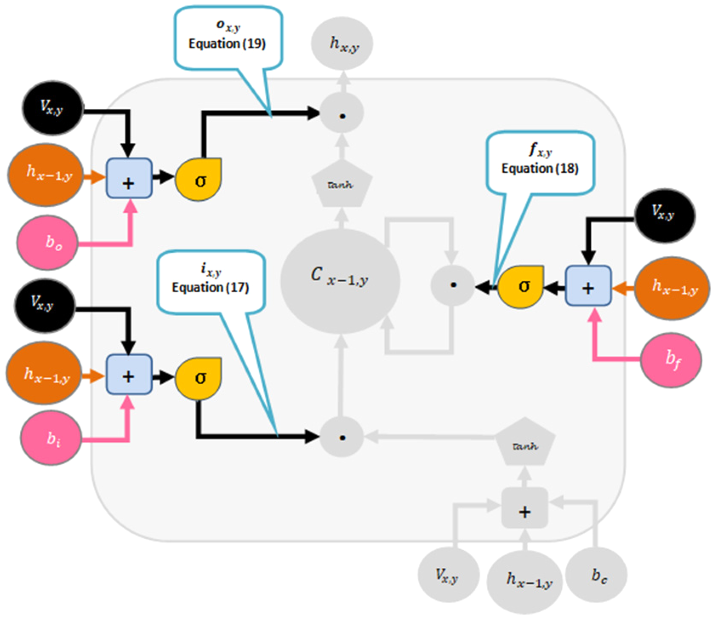
Computing update, forget and output gate in LSTM model.

The final output of the current cell for the x-th second of the y-th day is then calculated by using equation (20). To force the values to be between 1 and −1, tanh function is used. Then, the result are multiplied by the output gate value to get the final output.

h_{x, y} = o_{x, y} \cdot \tanh (c_{x, y})

(20)

For the x-th second in the y-th day, the outputs of the input are used, while gates output are neglected in order to realise the long-term patterns among PV power outputs across two days as below.

c_{x, y} = f_{x, y} \cdot c_{x - 1, y} + {\tilde{c}}_{x, y} i_{x . y}

(21)

Here the weighted sum for the current inputs for the current time step and the output of the previous second are calculated as follows.

{\tilde{c}}_{x, y} = \tanh (w_{v_{x, y} c} v_{x, y} + w_{h_{c}} h_{x - 1, y} + b_{c})

(22)

Figure 6 shows the output of the current cell, long term pattern and the pre-long term pattern which is calculated based on the current observation and the short term pattern for the previous second.

Figure 6.

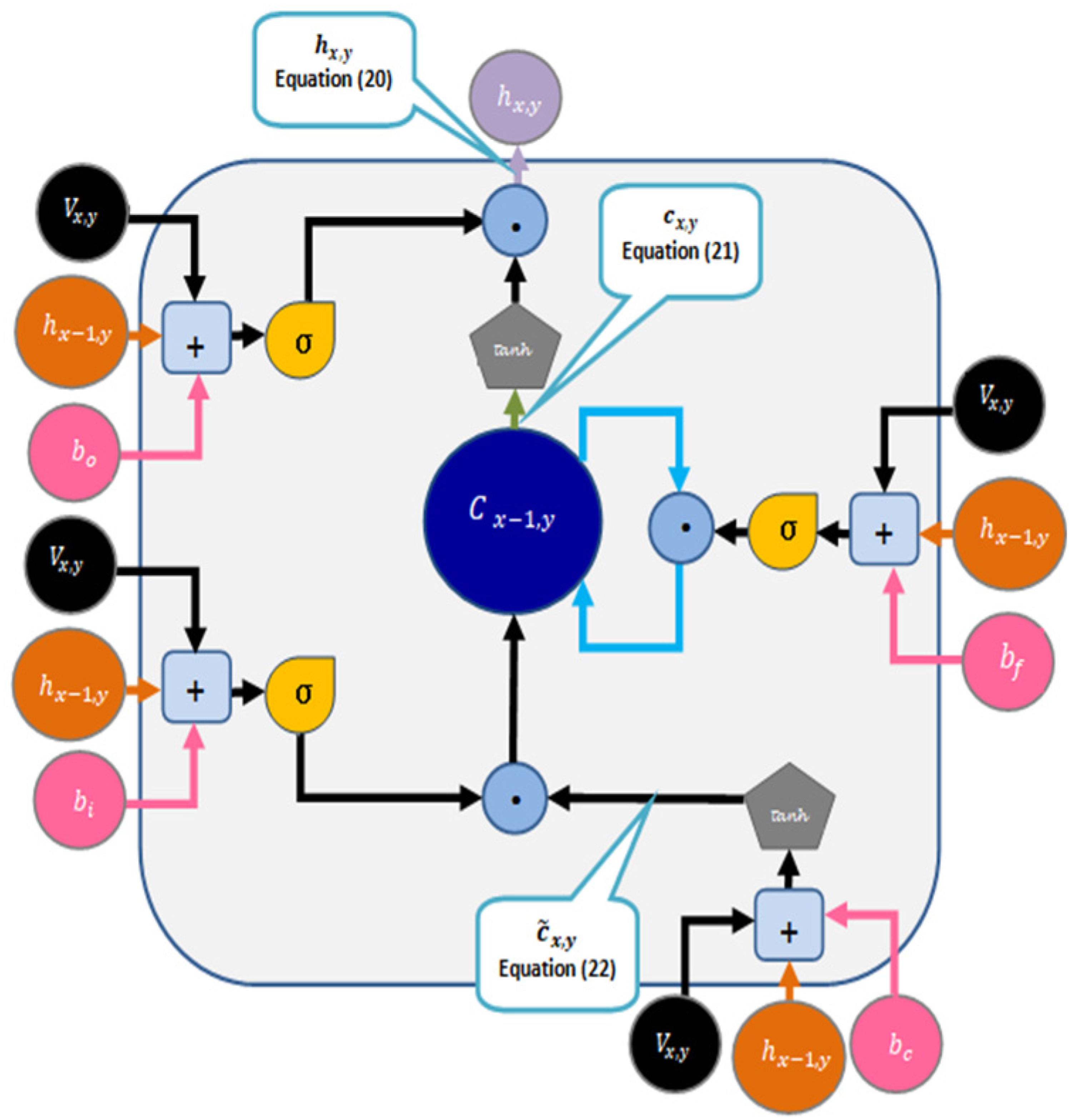
Computing the output of the current cell in LSTM model.

GRU-Based PV output current prediction

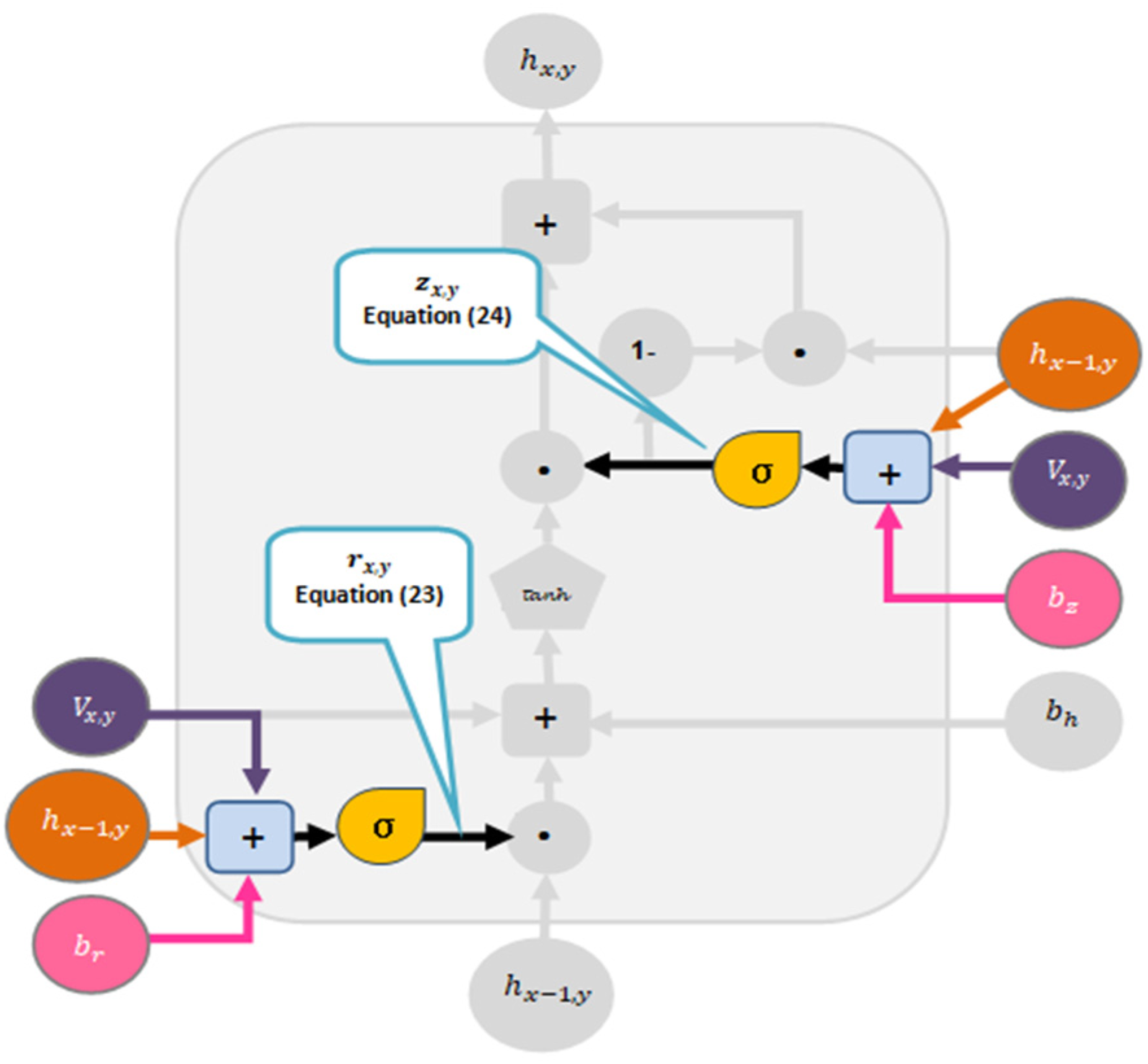
Figure 7 shows the construction for the x-th second in the y-th day. It consists of two gates which are reset and update gates which are denoted as $r_{x, y}$ and $z_{x, y}$ , respectively. Here $h_{x, y}$ means the current cell state. In addition, $b_{r}$ and $b_{z}$ are bias vectors. $w_{h_{r}}$ and $w_{h_{z}}$ are weight matrices for the reset and the update gates respectively. Sigmoid function is also applied here for the weighted summations of the inputs, the past outputs and the bias values for each gate. This is to calculate the output for each of the two gates through two steps.

Figure 7.

Block cell structure of the proposed GRU model.

The output of the reset gate which indicates how much unimportant information from previous cell that is needed to be forgotten is calculated first by using equation (23).

r_{x, y} = σ (w_{v_{x, y} r} v_{x, y} + w_{h_{r}} h_{x - 1, y} + b_{r})

(23)

Meanwhile, the output of the update gate which is a tremendous for determining how much information from the previous time step is required to pass through the future cells is calculated by using equation (24).

z_{x, y} = σ (w_{v_{x, y} z} v_{x, y} + w_{h_{z}} h_{x - 1, y} + b_{z})

(24)

Figure 8 shows the inputs for both the reset and the update gates.

Figure 8.

Computing the update and reset gates in GRU model.

Based on equation (25), the value of the reset gate that is used to know how much information is taken from the previous cell and use it as new memory content is used. After that, the weighted sum for the input $v_{x, y}$ and the previous cell state $h_{x - 1, y}$ are calculated. Finally, the nonlinear function $\tanh ()$ is applied.

{\tilde{h}}_{x, y} = \tanh (w_{v_{x, y} h} v_{x, y} + w_{h_{h}} h_{x - 1, y} + b_{h F})

(25)

h_{x, y}

is calculated by equation (26). This value determines how much information is required to obtain from previous time step

h_{x - 1, y}

and from the current cell block

h_{x, y} = (1 - z_{x, y}) \cdot h_{x - 1, y} + z_{x, y} \cdot {\tilde{h}}_{x, y}

(26)

Figure 9 shows the calculations for the output vector (

h_{x, y}

) and the candidate activation vector (

{\tilde{h}}_{x, y}

Figure 9.

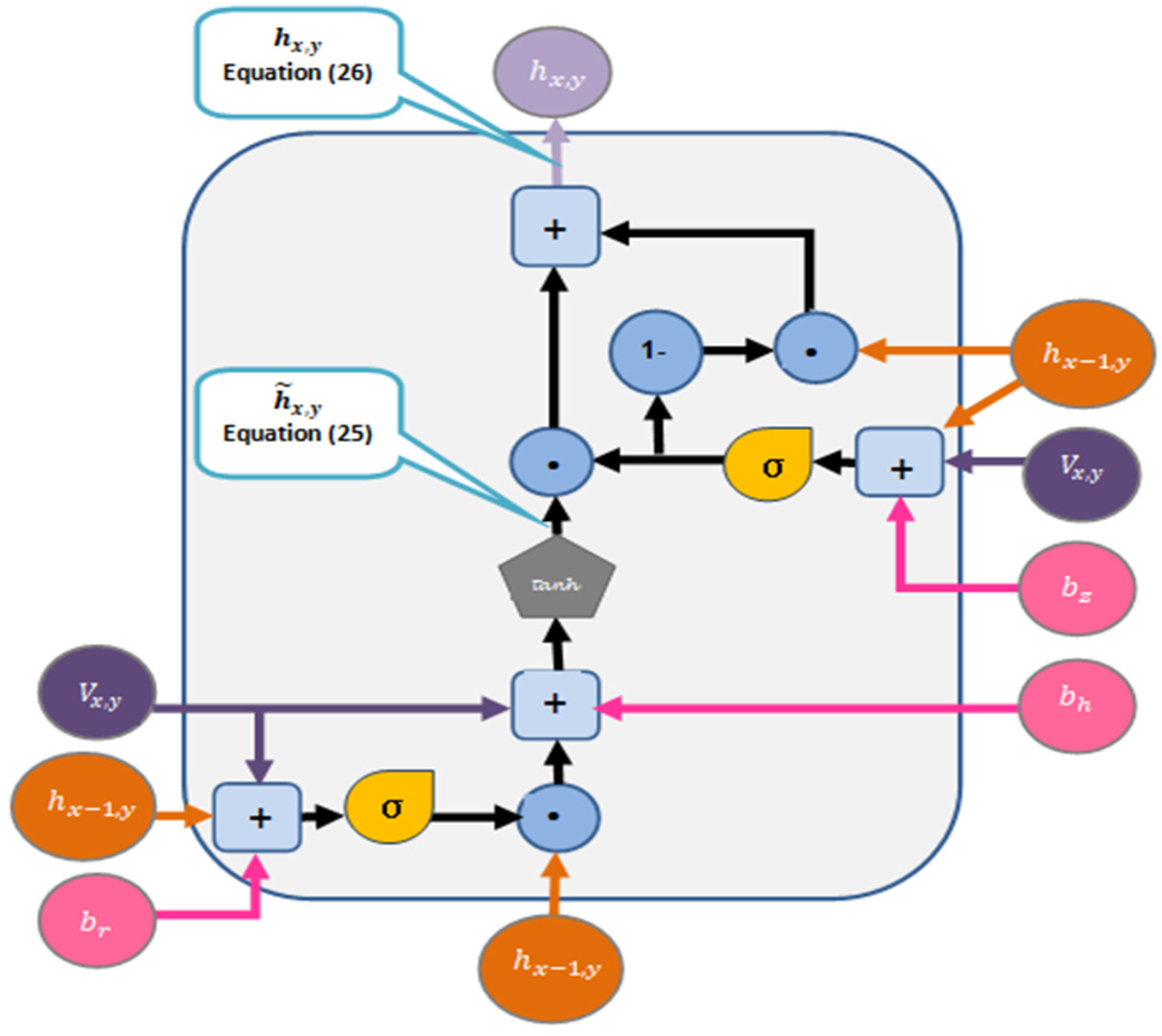
Computing the output of the current cell in GRU model.

Proposed models development

In this research, LSTM & GRU methods are implemented by using python as it is considered to be the best for machine learning projects because of its simplicity, flexibility and its consistency of tremendous libraries for artificial intelligence and machine learning. The utilised computer kit consists of an Intel® Core™ i7-8565U CPU @ 1.80 GHz and 8 GB RAM. The proposed models are built by using some of the deep learning toolkits such as Numpy, Tensorflow, Keras, Pandas, Matplotlib, Pylab and Datetime.

Firstly, data preprocessing is done to make the data suitable for proposed model by removing all comas and converting data to matrix shape format. In this stage, data features are scaled to a range from 0 to 1 to achieve a better performance. Afterwards, two arrays are created; one is called X_train and the other y_train. X_train consists of number of samples (rows) that is used for training, the number of left rows and the number of inputs. Meanwhile, y_train consists of the number of samples (rows) that is left after taking the samples that are used in training (the same of the second number that used in X_train array) and the number of outputs. Then the neural network is initialised by adding one hidden layer which is defined with 100 neurons. In addition, a regulation technique that is called Dropout with dropout rate equals to 0.25 so as to prevent model from overfitting is used. The model is compiled with the efficient Adam version of stochastic gradient descent and linear activation function. It is also fitted with 10 training epochs and a batch size 256. After that, selecting features process is started (columns) to be involved into training and prediction which are solar radiation, ambient temperature and photovoltaic system output current. After finishing training, future prediction is started for specified period which is considered as a parameter in date_range() function and then compared the results of prediction with the actual values.

Proposed model evaluation

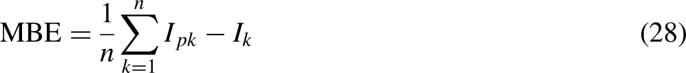
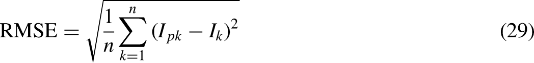
In this research R-Squared error, mean absolute error (MAPE), mean bias error (MBE) and root mean squared error (RMSE) are used to evaluate the proposed models. MAPE indicates model's general accuracy, where it can be calculated by comparing the measured values of the current with the predicted values of the current at specific test conditions. MAPE is computed by,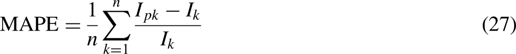

MAPE = \frac{1}{n} \sum_{k = 1}^{n} \frac{I_{p k} - I_{k}}{I_{k}}

(27)

Meanwhile, MBE provides information about the long-term performance of the proposed method and it shows the average variance between the predicted values of the current to the corresponding values of the real current. A positive MBE error means overestimation of data from datasets and vice versa. MBE can be determined using the equation below,

MBE = \frac{1}{n} \sum_{k = 1}^{n} I_{p k} - I_{k}

(28)

Eventually, RMSE is a measure of the variance of the current values from the model around the values of the real current, and it provides information on the short-term performance. RMSE is calculated by,

RMSE = \sqrt{\frac{1}{n} \sum_{k = 1}^{n} {(I_{p k} - I_{k})}^{2}}

(29)

where

I_{p k}

is the predicted current,

I_{k}

is the current measured value, and n is the number of data points.

Results and discussion

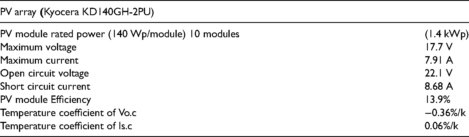
In this research, experimental data of a 1.4 kWp PV system are utilised in developing the proposed models. The specifications of the adopted system are as shown in Table 2. The performance of the system (output current and voltage) is recorded every one second. The monitoring system consists of solar radiation transmitter of high-stability silicon photovoltaic detector model WE300 with accuracy of ±1%, temperature sensor for the surface of the PV panel model WE710 with accuracy of ±0.25°C, air temperature sensor model WE700 with range of −50°C to +50°C and accuracy of ±0.1°C, and current transducer Model: CTH-050 with input range of 0–50 A (DC) and output of 4–20 mA.

Table 2.

Specifications of the PV system that is adapted in this research.

PV array (Kyocera KD140GH-2PU)
PV module rated power (140 Wp/module) 10 modules	(1.4 kWp)
Maximum voltage	17.7 V
Maximum current	7.91 A
Open circuit voltage	22.1 V
Short circuit current	8.68 A
PV module Efficiency	13.9%
Temperature coefficient of Vo.c	−0.36%/k
Temperature coefficient of Is.c	0.06%/k

On the other hand, Table 3 shows the adapted cases in this research, while, Figure 10 shows the profiles that are used in training the proposed model for each case.

Figure 10.

Training datasets for all testing cases. (a) Training data for case 1, (b) Training data for case 2 and 4, (c) Training data for case 3, (d) Training data for case 5 and 8, (e) Training data for case 6, (f) Training data for case 7.

Table 3.

Selected cases for training and testing the proposed models.

Case	Description
Case 1	Uncertain day for training, two stable days for testing
Case 2	Uncertain day for training, two uncertain days for testing
Case 3	Stable day for training, two uncertain day for testing
Case 4	Uncertain day for training, one week for testing
Case 5	Half of uncertain day, two uncertain days for testing
Case 6	Half of uncertain day, two stable days for testing
Case 7	Half of stable day for training, two uncertain day for testing
Case 8	Half of uncertain day, one week for testing

Figures 11 and 12 show the prediction results for both models and all cases. From the figures, it seems that both models could predict the photovoltaic output current accurately. However, in order to validate the results the evaluation metrics adapted in this research are presented in Tables 4 and 5.

Figure 11.

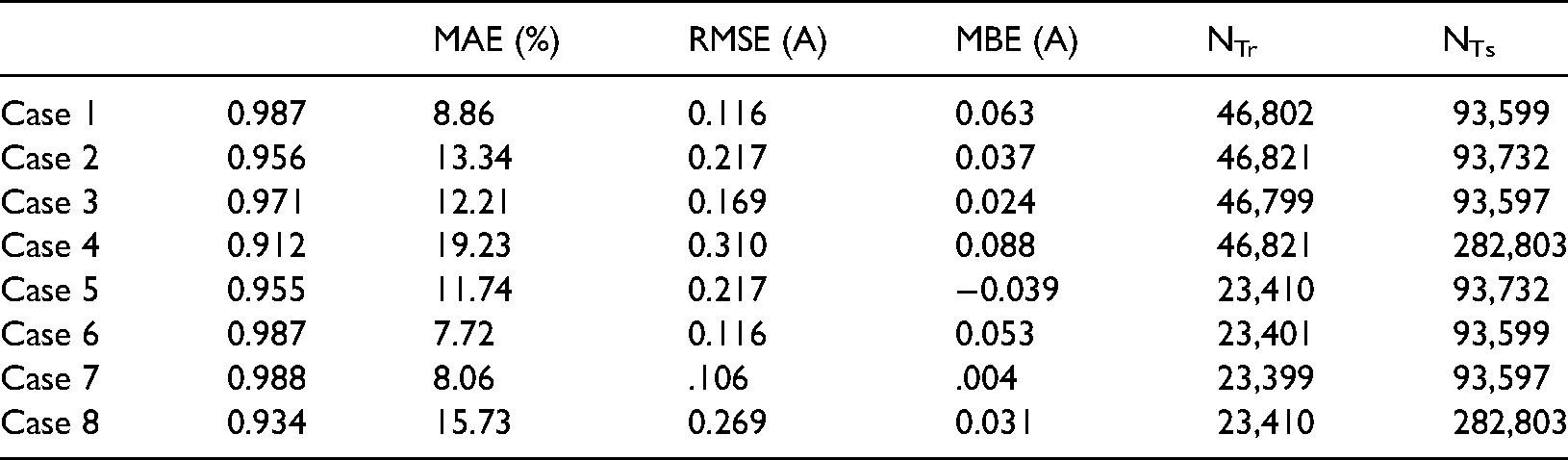
GRU results for PV ouput current prediction using different traning and testing sets.

Figure 12.

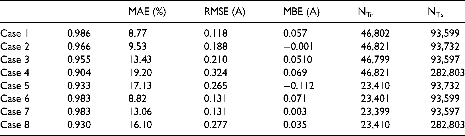
LSTM results for PV ouput current prediction using different traning and testing sets.

Table 4.

Evaluation of the proposed GRU model.

	$R^{2}$	MAE (%)	RMSE (A)	MBE (A)	N_Tr	N_Ts
Case 1	0.987	8.86	0.116	0.063	46,802	93,599
Case 2	0.956	13.34	0.217	0.037	46,821	93,732
Case 3	0.971	12.21	0.169	0.024	46,799	93,597
Case 4	0.912	19.23	0.310	0.088	46,821	282,803
Case 5	0.955	11.74	0.217	−0.039	23,410	93,732
Case 6	0.987	7.72	0.116	0.053	23,401	93,599
Case 7	0.988	8.06	.106	.004	23,399	93,597
Case 8	0.934	15.73	0.269	0.031	23,410	282,803

Table 5.

Evaluation of the proposed LSTM model.

	$R^{2}$	MAE (%)	RMSE (A)	MBE (A)	N_Tr	N_Ts
Case 1	0.986	8.77	0.118	0.057	46,802	93,599
Case 2	0.966	9.53	0.188	−0.001	46,821	93,732
Case 3	0.955	13.43	0.210	0.0510	46,799	93,597
Case 4	0.904	19.20	0.324	0.069	46,821	282,803
Case 5	0.933	17.13	0.265	−0.112	23,410	93,732
Case 6	0.983	8.82	0.131	0.071	23,401	93,599
Case 7	0.983	13.06	0.131	0.003	23,399	93,597
Case 8	0.930	16.10	0.277	0.035	23,410	282,803

Tables 4 and 5 show evaluation of the proposed models based on the adapted three statistical errors. From Table 4, the MAE of the proposed GRU accuracy is in the range of (7.7–19.2)% for all cases. The worst case is Case 4 when an uncertain day is used for training. Meanwhile, the best is when half of unstable day is used for training in order to predict two stable days. Here MAE results cannot be conclusive for these cases as it is somehow close and varying depending on day profile. However what we can read from MAE values that when profile (b) in Figure 10 is used for training, the worst results are obtained. As for the RMSE and MBE values, the situation is somehow close the MAE values whereas the RMSE values are in the range of 0.12–0.30 A, while MBE values are in the range of (−0.04–0.9) A respectively. Both RMSE and MBE show acceptable accuracy for both models. However, in this research the focus is given to Case 4 and Case 8. In these cases the relatively high MAE is noted because of the night time values between the days and therefore, the focus is given more to the RMSE and MBE to evaluate these cases. The RMSE and MBE are better for Case 8 although less data are used for training. This is mainly because of the utilised profile for training. Although the same day was used for the training, but it is very clear that the morning (1^st half of the day) is better than the 2^nd half whereas current values are reduced very much. This means that the profile of the first half of the day is more consistent and therefore, the results were better for this part.

As for LSTM model, Table 5 shows somehow similar scenario and analysis to the GRU model whereas the range of MAE, RMSE and MBE values are (8.9–19.2)%, (0.12–0.32) A and (−0.002–0.071) A respectively. Here also results of Case 8 are slightly better than results of Case 4.

Anyway, with both models, case 8 (the preferred case) accuracy is very close to the results of other cases and thus, it is possible to consider the use of half of a day for training is enough for one week time prediction considering highly sensitive data.

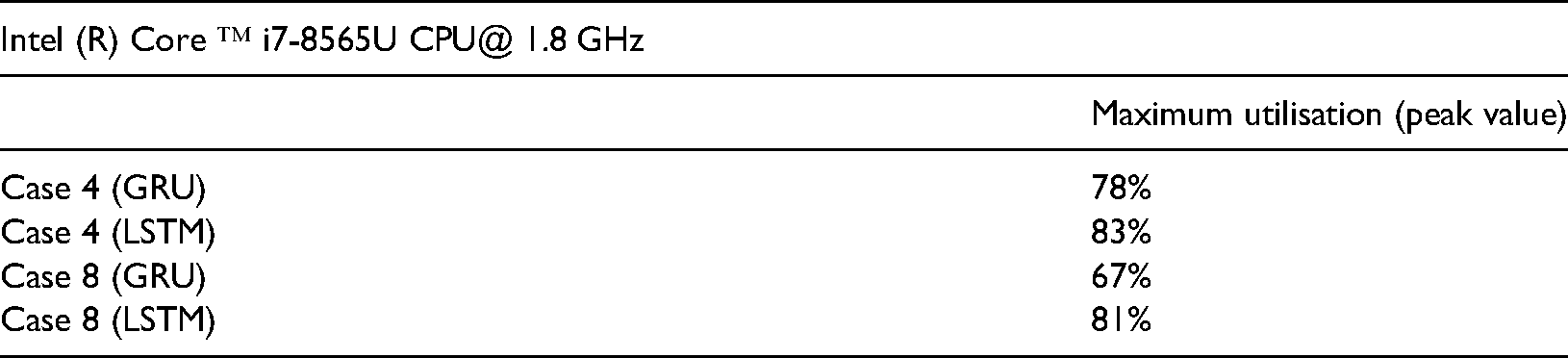
Table 6 shows the utlization of the processor based on the case and the utlizated model. In fact, it is expected that as far as, the required training data is smaller, the utlization of the processor is lower. This means less required computunal power and consquently esier to embed the model on controller as a physical system. In Table 6, Case 4 means that one day is used for training, meanwhile, case 8 means that only half a day is used for training. From the table, Case 8 utlized less than Case 4 of the processor meanwhile GRU model requires less power than LSTM to exctute the process. Therefore, GRU is prefered for such a task as it is slightly more accurate than LSTM and requires less computional power.

Table 6.

Computational power required for PV output power prediction by using GRU and LSTM model.

Intel (R) Core ™ i7-8565U CPU@ 1.8 GHz
	Maximum utilisation (peak value)
Case 4 (GRU)	78%
Case 4 (LSTM)	83%
Case 8 (GRU)	67%
Case 8 (LSTM)	81%

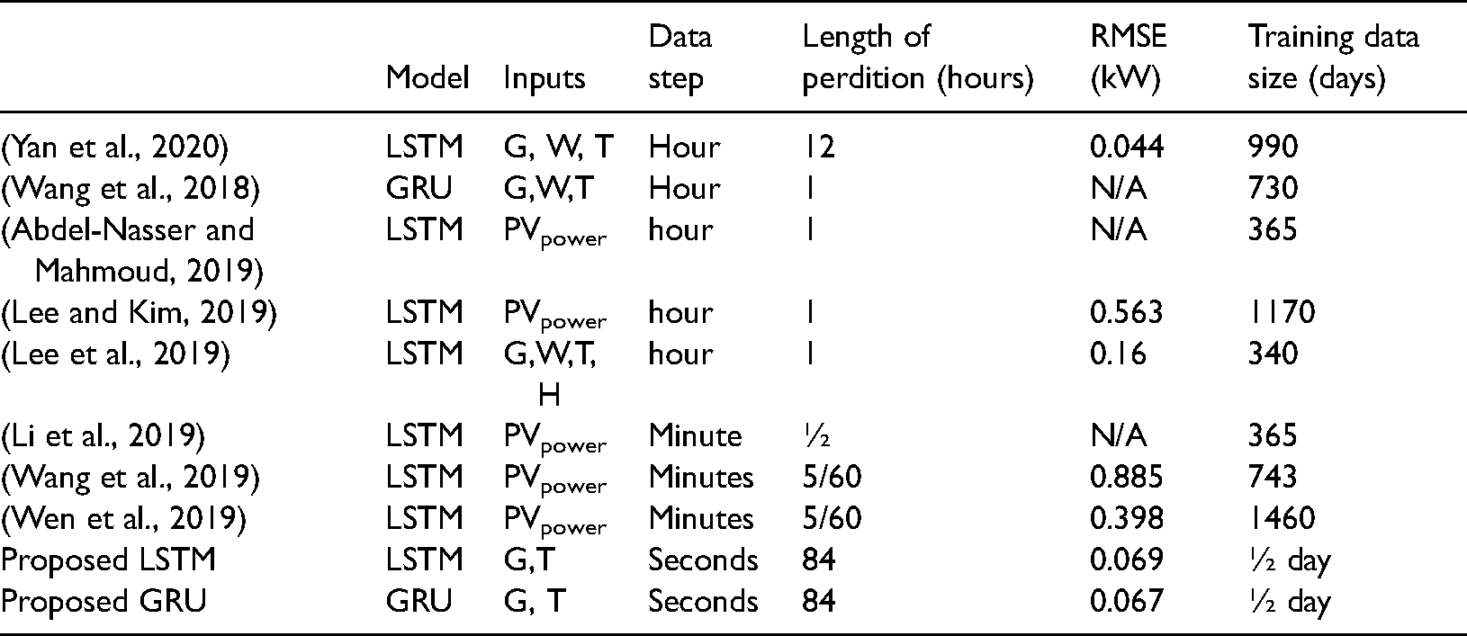
To present the results of the proposed models in a better way, a comparison with methods presented in (Abdel-Nasser and Mahmoud, 2019; Lee et al., 2019; Lee and Kim, 2019; Li et al., 2019; Wang et al., 2018, 2019; Wen et al., 2019; Yan et al., 2020) is conducted in Table 7. The comparison is done considering number and types of inputs (G: solar radiation, T: ambient temperature, W: wind speed, H: relative humidity), required data for training, length of predicted data, type of the model, and sensitivity of the data utilised. From the table the proposed models have used the minimum training data to predict the maximum period at the best accuracy. This is because of the utilisation of high sensitive data (in seconds), whereas models are able to learn in much better way than models that are developed based on datasets in minutes or hours.

Table 7.

Comparison between the proposed models and other similar models.

	Model	Inputs	Data step	Length of perdition (hours)	RMSE (kW)	Training data size (days)
(Yan et al., 2020)	LSTM	G, W, T	Hour	12	0.044	990
(Wang et al., 2018)	GRU	G,W,T	Hour	1	N/A	730
(Abdel-Nasser and Mahmoud, 2019)	LSTM	PV_power	hour	1	N/A	365
(Lee and Kim, 2019)	LSTM	PV_power	hour	1	0.563	1170
(Lee et al., 2019)	LSTM	G,W,T,H	hour	1	0.16	340
(Li et al., 2019)	LSTM	PV_power	Minute	½	N/A	365
(Wang et al., 2019)	LSTM	PV_power	Minutes	5/60	0.885	743
(Wen et al., 2019)	LSTM	PV_power	Minutes	5/60	0.398	1460
Proposed LSTM	LSTM	G,T	Seconds	84	0.069	½ day
Proposed GRU	GRU	G, T	Seconds	84	0.067	½ day

Conclusion

In this research, two deep learning neural network models were proposed to predict photovoltaic output current. The proposed models were long short-term memory and gated recurrent unit neural networks. The proposed models were developed based on minimum data for training so as to predict one week time by utilising performance datasets in seconds for a PV system. The proposed model is assumed to predict photovoltaic output current at each second for one week time by using global solar radiation and ambient temperature values as inputs. Python environment were used to develop the proposed models, while, three statistical errors were used to evaluate the proposed models which were mean absolute percentage error, root mean square error and mean bias error. Results showed that the proposed model could accurately predict photovoltaic output current whereas the root mean square error values are in the range of 0.12–0.30 A, while mean bias error values were in the range of (−0.04–0.9) A for the proposed GRU model. Meanwhile root mean square error and mean bias error values were (8.9–19.2)%, (0.12–0.32)A and (−0.002–0.071) A respectively. Based on that, it was concluded that GRU is better than LSTM as it could predict photovoltaic output current slightly better. GRU it utilised less capacity of the utilised processor as compared to LSTM. Finally a comparison with other similar methods was conducted so as to show the significance of the proposed models. Based on this comparison, the utilisation of highly sensitive data (in seconds) made the proposed model more accurate in predicting targets as the utilisation of such data made the learning process of the machines more efficient.

Footnotes

Declaration of conflicting interests

The author(s) declared no potential conflicts of interest with respect to the research, authorship, and/or publication of this article.

Data Availability

Data is available upon request from the author.

Funding

The author(s) received no financial support for the research, authorship and/or publication of this article.

ORCID iDs

Tamer Khatib

Aladdin Masri

References

Abdel-Nasser

Mahmoud

(2019) Accurate photovoltaic power forecasting models using deep LSTM-RNN. Neural Computing and Applications 31: 2727–2740.

Ameen

Pasupuleti

Khatib

(2015) Modeling of photovoltaic array output current based on actual performance using artificial neural networks. Journal of Renewable and Sustainable Energy 7(5): 053107.

Aslam

Lee

Kim

, et al. (2019) Deep learning models for long-term solar radiation forecasting considering microgrid installation: A comparative study. Energies 13: 47.

Ayompe

Duffy

McCormack

, et al. (2010) Validated real-time energy models for small-scale grid-connected PV-systems. Energy 35: 4086–4091.

Bacher

Madsen

Nielsen

(2009) Online short-term solar power forecasting. Solar Energy 83: 1772–1783.

Bermejo

Gómez

Fernández , et al. (2019) A review of the use of artificial neural network models for energy and reliability prediction. A study of the solar PV, hydraulic and wind energy sources. Applied Sciences 9(9): 1844.

Brano

Ciulla

Falco

(2014) Artificial neural networks to predict the power output of a PV panel. International Journal of Photoenergy 2014: 1-13 (Article ID 193083).

Chow

Lee

(2012) Short-term prediction of photovoltaic energy generation by intelligent approach. Energy and Buildings 55: 660–667.

Cucumo

Rosa

Ferraro

, et al. (2006) Performance analysis of a 3 kW grid-connected photovoltaic plant. Renewable Energy 31: 1129–1138.

10.

Durisch

Bitnar

Mayor

, et al. (2007) Efficiency model for photovoltaic modules and demonstration of its application to energy yield estimation. Solar Energy Materials and Solar Cells 91: 79–84.

11.

Ghimire

Deo

Raj

, et al. (2019) Deep solar radiation forecasting with convolutional neural network and long short-term memory network algorithms. Applied Energy 253: 113541.

12.

Hammer

Heinemann

Lorenz

, et al. (1999) Short-term forecasting of solar radiation: A statistical approach using satellite data. Solar Energy 67: 139–150.

13.

Jie

, et al. (2020) Probabilistic solar irradiance forecasting via a deep learning-based hybrid approach. IEEJ Transactions on Electrical and Electronic Engineering 15: 1604–1612.

14.

Hove

(2000) A method for predicting long-term average performance of photovoltaic systems. Renewable Energy 21: 207–229.

15.

Jeon

Kim

(2020) Next-Day prediction of hourly solar irradiance using local weather forecasts and LSTM trained with Non-local data. Energies 13: 5258.

16.

Khatib

Elmenreich

(2016) Modeling of Photovoltaic Systems Using MATLAB: Simplified Green Codes (1st ed.). New Jersey, US: John Wiley & Sons, 240.

17.

Lee

Kim

(2019) Recurrent neural network based hourly prediction of photovoltaic power output using meteorological information. Energies 12(2): 15. Energies 2020, 13, 6623 23 of 23

18.

Lee

Jeong

Yoon

, et al. (2019) Improvement of short-term BIPV power predictions using feature engineering and a recurrent neural network. Energies 12: 3247.

19.

Shu

(2014) An ARMAX model for forecasting the power output of a grid connected photovoltaic system. Renewable Energy 66: 78–89.

20.

Wang

Zhang

, et al. (2019) Recurrent neural networks based photovoltaic power forecasting approach. Energies 12: 2538.

21.

Navabi

Abedi

Hosseinian

, et al. (2015) On the fast convergence modeling and accurate calculation of PV output energy for operation and planning studies. Energy Conversion and Management 89: 497–506.

22.

Qing

Niu

(2018) Hourly day-ahead solar irradiance prediction using weather forecasts by LSTM. Energy 148: 461–468.

23.

Ran

Guangmin

(2008) Photovoltaic power generation output forecasting based on support vector machine regression technique. Electric Power 41: 74–78.

24.

Sharadga

Hajimirza

Balog

(2020) Time series forecasting of solar power generation for large-scale photovoltaic plants. Renewable Energy 150: 797–807.

25.

Sulaiman

Rahman

Musirin

, et al. (2012) An artificial immune-based hybrid multi-layer feedforward neural network for predicting grid-connected photovoltaic system output. Energy Procedia 14: 260–264.

26.

Wang

Liao

Chang

(2018) Gated recurrent unit network-based short-term photovoltaic forecasting. Energies 11: 2163.

27.

Wang

Liu

(2019) A comparison of day-ahead photovoltaic power forecasting models based on deep learning neural network. Applied Energy 251: 113315.

28.

Wang

Zhen

, et al. (2015) Yang G. Solar irradiance feature extraction and support vector machines based weather status pattern recognition model for short-term photovoltaic power forecasting. Energy and Buildings 86: 427–438.

29.

Wen

Zhou

Yang

, et al. (2019) Optimal load dispatch of community microgrid with deep learning based solar power and load forecasting. Energy 171: 1053–1065.

30.

Wojtkiewicz

Hosseini

Gottumukkala

, et al. (2019) Hour-ahead solar irradiance forecasting using multivariate gated recurrent units. Energies 12: 4055.

31.

Wong

Wan

Lam

(2010) Artificial neural networks for energy analysis of office buildings with daylighting. Applied Energy 87: 551–557.

32.

Yan

Shen

Wang

, et al. (2020) Short-term solar irradiance forecasting based on a hybrid deep learning methodology. Information 11: 32.

33.

Yang

Huang

, et al. (2014) A weather-based hybrid method for 1-Day ahead hourly forecasting of PV power output. IEEE Transactions on Sustainable Energy 5(3): 917–926.

34.

Cao

Zhu

(2019) An LSTM short-term solar irradiance forecasting under complicated weather conditions. IEEE Access 7: 145651–145666.

35.

Zang

Liu

Sun

, et al. (2020) Short-term global horizontal irradiance forecasting based on a hybrid CNN-LSTM model with spatiotemporal correlations. Renewable Energy 160: 26–41.

Novel models for photovoltaic output current prediction based on short and uncertain dataset by using deep learning machines

Abstract

Keywords

Introduction

Photovoltaic output current characteristics and models

Proposed deep learning machines models

LSTM-Based PV output current prediction

GRU-Based PV output current prediction

Proposed models development

Proposed model evaluation

Results and discussion

Conclusion

Footnotes

Declaration of conflicting interests

Data Availability

Funding

ORCID iDs

References