Data Science in the Research Domain Criteria Era: Relevance of Machine Learning to the Study of Stress Pathology,Recovery,and Resilience

Abstract

Diverse environmental and biological systems interact to influence individual differences in response to environmental stress. Understanding the nature of these complex relationships can enhance the development of methods to (1) identify risk, (2) classify individuals as healthy or ill, (3) understand mechanisms of change, and (4) develop effective treatments. The Research Domain Criteria initiative provides a theoretical framework to understand health and illness as the product of multiple interrelated systems but does not provide a framework to characterize or statistically evaluate such complex relationships. Characterizing and statistically evaluating models that integrate multiple levels (e.g. synapses, genes, and environmental factors) as they relate to outcomes that are free from prior diagnostic benchmarks represent a challenge requiring new computational tools that are capable to capture complex relationships and identify clinically relevant populations. In the current review, we will summarize machine learning methods that can achieve these goals.

Introduction

The Research Domain Criteria (RDoC) conceptualizes mental health and mental illness as the result of multiple overlapping and interdependent dimensions.^1,2 This framework provides significant opportunity for advances in research into stress psychopathology and stress resilience as the etiology of such responses are, by definition, due to interactions between diverse internal and external factors. Empirically, biological systems that relate to stress pathology such as HPA axis regulation,^3,4 immune functioning,^5,6 the renin–angiotensin system, ⁷ the sympathetic–adrenal–medullary system, ⁸ and circadian rhythms^9,10 are known to have multiple overlapping components spanning from genes to neurocircuits. ¹¹ Further, these systems affect each other in complex, often multidirectional, ways across the central and peripheral nervous systems both in response to prior and current stress, daily demands, and internal rhythms.^11–19 Integrating information across these dimensions to make clinical decisions about an individual patient represents a significant challenge that may be necessary to overcome to advance therapeutics.

The RDoC initiative not only encourages a reconceptualization of the factors that impact health and psychopathology but also encourages a rethinking of the primary outcomes under study with explicit direction to move away from diagnostic classification.^1,2 Stress can produce temporary or even permanent alterations in cognition, ²⁰ memory, ²¹ arousal, ²² sleep,^9,10 mood, ²³ motor activity, ²⁴ and approach/avoidance behaviors. ²⁵ Examining such behaviors as the primary outcome makes sense as psychiatric diagnoses aggregate diverse presentations resulting in diagnoses that can encompass vast clinical presentations making them too heterogeneous to be useful as research tools. ²⁶

Characterizing health and pathology and uncovering mechanisms underlying these outcomes without the traditional mile markers of psychiatric diagnosis presents with a significant conceptual and computational challenge. The limited guidance that has been given as part of the RDoC initiative regarding computational methods is that “Most important, this framework needs to integrate many different levels of data to develop a new approach to classification based on pathophysiology and linked more precisely to interventions for a given individual.” ² Machine learning (ML) approaches are designed to achieve these goals.

ML methods can be cast into three general categories: (1) Unsupervised methods, which describe a class of algorithms that find relationships between variables without reference to a specific outcome. Unsupervised learning models provide information about how variables cluster together or relate to each other without an explicit outcome of interest. (2) Supervised models are designed to predict or classify an outcome of interest such as the presence or absence of a mental disorder. (3) Reinforcement learning (RL) examines how actions in one’s environment (such as treatment) alter behavioral states. These methods provide a powerful set of tools to examine mechanisms, predict risk, and develop treatment based on complex sources of information. In this review, we will focus on computational methods and examples from stress pathology research that attempt to achieve these goals. The goal of this review is to provide a broad overview of ML concepts and their relevance to stress pathology research in the RDoC era.

What Is Machine Learning?

ML refers to a large class of algorithms that attempt to learn patterns from data to improve performance and make predictions. ²⁷ Such algorithms recursively search for relationships in data by applying a set of logical rules and mathematical tools. Because such algorithms are powerful tools for identifying relationships between variables, ML methods are prone to overfitting or fitting a model that is specific to the data at hand but is not generalizable. For this reason, ML algorithms also integrate safeguards against overfitting.

There are many different algorithms that are designed to achieve the same general goals (i.e. supervised, unsupervised, and RL). No single algorithm works best in all contexts. Often data scientists will compare results from a number of different algorithms or select one based on specific needs. For example, ML approaches vary in their interpretability. In many nonscientific contexts, data analysts may be less concerned with interpretation compared to model building. A stockbroker attempting to predict if the Dow Jones will increase in the next quarter may fit a model to make a decision about the likely course of the market without much interest in the nature of the underlying relationships that lead the Dow to increase or decrease. However, an economist investigating the same question may be much more interested in underlying the factors that lead to the outcome. Methods such as support vector machines (introduced below) are powerful methods for predictive modeling but are known as a “black box” because the nature of the underlying relationships is not accessible. Conversely, methods such as graph models (also introduced below) are highly interpretable but their stability and accuracy for decision-making can be limited. As such, when choosing a modeling approach, data scientists often weigh their goals in terms of the need to interpret and the need to build a stable model.

A general strength of ML methods is their ability to integrate larger sets of variables and capture complex dependencies between variables. ML methods can model dependencies between variables using Boolean logic (AND, OR, NOT), absolute conditionality (IF, THEN, ELSE), and conditional probabilities (probability of X given Y). Such an approach allows models to capture multiple dependent relationships and, as such, have increased relevance to real-world scenarios where multiple factors are in play. In the context of stress pathology such as posttraumatic stress disorder (PTSD), for example, multiple risk factors have been identified but none robustly predict risk alone. ²⁹ This may indicate that multiple factors work together and/or risk factors vary between individuals.

Female gender is a case in point as it has consistently been replicated as a risk factor for PTSD but only accounts for a small percentage of variance and is only relevant to some who develop the disorder. ³⁰ Recent findings in endocrinology, genetics, and epigenetics help to explain why female gender increases risk as the role of estrogen signaling in HPA axis regulation has come into focus,^31–34 indicating that risk associated with female gender may be nested in underlying biological functions related to estrogen signaling. Indeed, women have been shown to vary in their risk for PTSD depending on when in their cycle they experience a traumatic event. ³⁵ Finally, the different causes of stress-related pathology may not be reducible to biological explanations alone. Early environment has been shown to permanently alter HPA axis functioning. ³⁶ Like many biological systems, these dependencies are fundamentally nonlinear, ³⁷ creating a need to characterize complex nonlinear relationships. ML methods can be utilized to build models based on such complex environmental and biological dependencies to make predictions about risk in future cases.

Bayesian Estimation

The backbone of traditional statistical theory and associated statistical tests is the goal of null hypothesis testing which tests P(D|H₀) meaning the probability of the data given the assumption that the null hypothesis is true or that the assumption is that there are no relationships between the variables in the model. ³⁸ Null hypothesis testing is embedded in statistical theory as a safeguard against a priori assumptions about the nature of populations under study or their relationships to covariates. ³⁹ However, a consequence of this level of rigor is that researchers cannot use prior research to make estimates.

While this may seem like an esoteric statistical issue, it has real-life consequences for a researcher’s ability to develop methods for mechanism identification, prediction, and individualized treatment. ⁴⁰ In the context of a treatment study, for example, the null hypothesis is that the treatment has no effect greater than chance. This rigorous assumption is useful when examining a novel treatment. But when a treatment has demonstrated a consistent but moderate effect, such as exposure therapy for phobias and PTSD, researchers may turn their attention from the question of if exposure therapy has an effect to research aimed at determining for whom does the treatment have an effect. The latter research question is outside of the realm of null hypothesis testing because such models make assumptions based on previous data that the treatment is effective in some cases and that success is dependent on some factors. To make a decision about the probability of successful treatment given, some individual characteristics require assumptions about future events given past information. Such questions can be mathematically formulated using Bayes theorem.

Bayes’ theorem states that $\text{P}(\text{A}|\text{B})=\frac{\text{P}(\text{B}|\text{A})\text{P}(\text{A})}{\text{P}(\text{B})}$ . This simple formula provides a method to estimate the posterior probability of one occurrence given another. For example, prior research has demonstrated that the BDNF val66/met polymorphism is associated with recovery in exposure therapy. ⁴¹ These findings can be translated using Bayes theorem to calculate the probability of recovery given that the patient is a Val66/met carrier as

$$\begin{array}{c}\multicolumn{1}{c}{\text{P}(\text{Recovery}|\text{Val}66/\text{met})}\\ \multicolumn{1}{c}{=\frac{\text{P}(\text{Val}66/\text{met}|\text{Recovery})\text{P}(\text{Recovery})}{\text{P}(\text{Vol}66/\text{met})}}\end{array}$$

An additional benefit of Bayesian estimation is that it greatly simplifies estimation, allowing for the integration of more variables with fewer subjects. ⁴² To illustrate this, imagine that you sit down to watch TV when you realize you have lost the remote. A null hypothesis test would use frequentist methods such as maximum likelihood estimation ⁴³ that make no assumptions about where the remote control might be. Following this school of thought, you would sample, or look any physical space, that the remote could fit in. This rigorous approach would assume an equal probability that the remote control is in the oven or under the bed as it is to be jammed in the sofa cushion. Acting as a Bayesian, you would use prior knowledge to estimate a distribution related to the probability of the remote’s position. You may start in the three places the remote is most often and then radiate out to less probabilistic locations (e.g. the oven). This conception translated to research allows for much less sampling and computational effort to test the same hypotheses. Further, it allows for increased model complexity because researchers can state and test complex dependencies. For example, the distribution of locations of the remote control may change depending on who was last watching TV, and as such, you may make a different estimate that is informed by the probabilistic location given a particular individual.

Returning to exposure therapy, it is unlikely that the BDNF val66/met polymorphism alone will predict treatment success with high enough accuracy to make a treatment decision. However, researchers may improve prediction by integrating other relevant predictors that relate to the probability of treatment success. These predictors may be independent meaning that the probabilistic information they provide is independent of the genetic effect. Predictors can also be dependent in a manner that together provides as more accurate picture of the genetic risk. For example, the BDNF val66/met polymorphism is likely to affect the probability of recovery in exposure therapy because of its effect on BDNF protein synthesis, a growth factor involved in neurogenesis that affects learning and memory. The probabilistic estimate of recovery therefore may be enhanced by estimating the probability given the presence of val66/met, increases synthesis of BDNF, and increases in neurogenesis in relevant brain regions. Bayesian estimation provides a framework to build models based on prior experience (e.g. data) to make predictions about future cases.

Unsupervised Learning

Unsupervised learning refers to a class of algorithms that attempt to draw inferences about the relationship between variables in the absence of an outcome of interest.^28,44 For example, a researcher may want to determine physiological channels that cluster together in response to a stressor or regions of the brain that are coactivated to characterize brain circuits. Researchers may also want to define populations based on such clusters ⁴⁵ rather than relying on a priori definitions such as diagnostic status. This is of particular relevance in the RDoC era which does not rely on traditional psychiatric classification methods to define health and illness. Finally, unsupervised methods are also of value for data reduction. ⁴⁶ Data reduction methods allow data scientists to filter down from a very large set of variables. Such an approach is useful when working, for example, with genetic and epigenetic data where the variable count can be in the millions. ⁴⁷

Feature Selection and Feature Extraction

One common use of unsupervised learning method for data reduction is to reduce the dimensionality of a set of variables (or features) by removing redundant or irrelevant variables ⁴⁸ or by combining variables into composite values. ⁴⁹ Commonly in social and biological sciences, researchers are confronted with situations where a large number of variables may be of theoretical interest, but empirically, they are largely overlapping in the information that they provide. For example, cortisol and corticotropin-releasing hormone (CRH) are causally related to each other as CRH stimulates the production of cortisol. ⁵⁰ However, they may correlate to such a high degree that the information they provide is largely overlapping, or redundant. A researcher may want to down-select to reduce the number of variables in the model to guard against overfitting due to the curse of dimensionality whereby models become increasingly accurate in differentiating populations as the number of variables in the model increases. ⁵¹ Similarly, these two markers (CRH and cortisol) may cluster together while an additional marker, such as glucose, may not make glucose irrelevant as it is unrelated to the larger cluster of variables. Similarly, the researcher may want to down-select irrelevant variables to reduce dimensionality and ultimately reduce the changes of overfitting the model.

Feature selection is distinguished from another commonly used unsupervised method, feature extraction. ⁵² In this context, new, more stable, variables are created by combining variables or extracting the shared variance between variables. Returning to the example of physiological data measured in response to stress, a researcher may want to derive a single variable that represents the relationship between physiological measures. This can reduce the number of variables in a model and can also add stability in measurement. In this instance, researchers may use methods such as principle components analysis (PCA), ⁴⁹ which captures the shared variance between multiple variables which can ultimately be utilized as a variable in future analyses.

We provide a simple, illustrative example whereby a researcher wants to determine crime in his research subject’s neighborhood to use as a proxy measure for stress and danger in the subject’s environment. To achieve this, the researcher downloads crime statistics based on subject’s zip code, yielding multiple crime statistics including petty larceny, murder, rape, misdemeanor sex crimes among many others. This set is too large to analyze on its own, and further, any particular variable may not be very informative. As Figure 1 demonstrates, PCA can reduce dimensionality significantly to extract high variance components. In this case, two components were extracted that approximate violent crimes (i.e. assault, robbery, shootings, rape, and murder) and nonviolent crimes (i.e. misdemeanor sexual assault, loitering, and grand larceny). By reducing dimensionality in this way, researchers can then study a smaller set of variables that relate to broader constructs.

Figure 1.

Principle components analysis (PCA) of census crime statistics. The figure demonstrates a PCA of census data. Crime statistics demonstrated to primary principle components or sets of shared variance. Component 1, which primarily comprised variance from violent crimes, accounted for approximately 66.9% of the total variance while Component 2, which primarily comprised variance from nonviolent crimes, accounted for 21.5% of the total variance.

Population Clustering

Increasingly, researchers are interested in identifying populations empirically rather than relying on a priori definitions. To achieve this, researchers often attempt to identify individuals who cluster together into clinically relevant populations. By identifying such populations, researchers can then test hypotheses about them. This approach is particularly relevant in the RDoC era where researchers are discouraged from using diagnoses to define populations.

There are many methods to cluster populations. One commonly utilized approach is to identify latent or not directly observable populations by identifying underlying mixture distributions (i.e. mixture modeling). ⁵³ For example, Figure 2 demonstrates a bimodal observed distribution with two underlying latent normal distributions. This is refered to as a mixture distribution. ⁴⁵ Returning to the example of measurements of physiological arousal in response to a stressor, these distributions may capture low-arousal and high-arousal individuals. These populations may be of clinical relevence and can now be examined as an outcome in lew of diagnoses.

Figure 2.

Example of a two-mixture distribution. In this example, two latent (unobserved) distributions that are overlapping (mixture distributions) and that are both Gaussian normal (red and green) are identified underlying an observed nonnormal distribution (grey).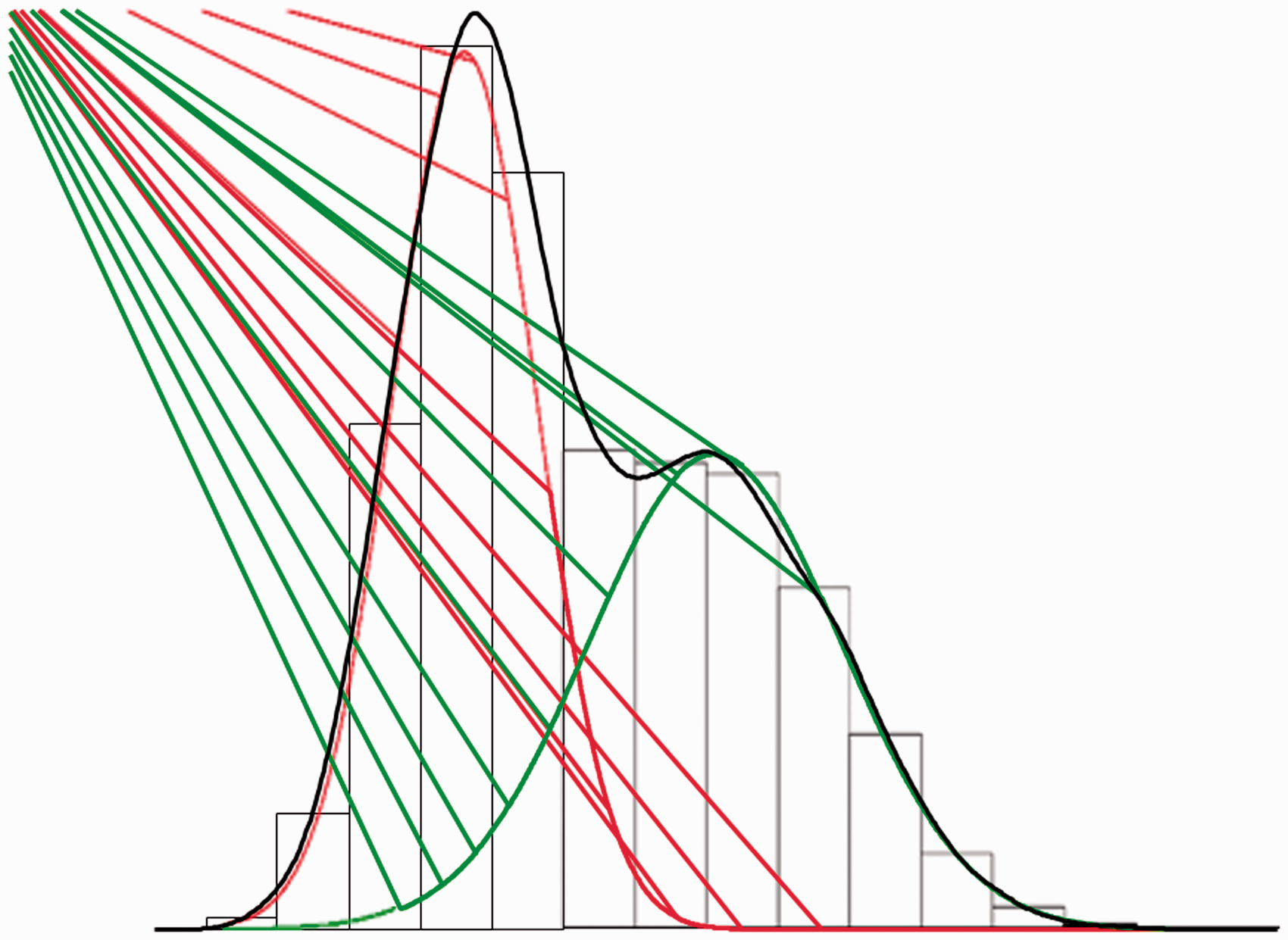

The general prinicple of mixture modeling can be extended to longidinal data to examine change over time. This approach is relevent when researchers hypothesize that populations are differentiated not only by their level of severity but also change. Returing to the example of physiological stress response data, researchers may be interested to know if there are distinct populations based on the ability to habituate to loud tones or to aquire and extinguish associations between conditioned and unconditioned stimuli as these both are models that are hypothesized to underly diverse stress pathologies.

Latent growth mixture modeling (LGMM) is one such approach that is commonly used in stress pathology research. ⁵⁴ This approach utilizes repeated measures to estimate a set of latent variables that indicate general levels on a particular variable (intercept parameter) and change across measurement occations (e.g. slope and quadratic parameters). From these variables, LGMM attempts to identify a second-order latent variable (class) which defines populations based on their similarities in the intercept, slope, and quadratic parameters. Figure 3 provides an example of trajectories derived based on eyeblink startle in response to threat (fear) acquisition and extinction training. ⁵⁵ In this example, by first identifying distinct trajectories in acquisition and extinction learning, researchers were able to determine the relationship between individual’s trajectory during extinction learning and risk genes as well as clinical presentation.

Figure 3.

Three class latent growth mixture modeling (LGMM) of fear conditioning and extinction learning. Binned observations of eyeblink startle response are examined in response to a blue square paired with an air blast to the larynx (acquisition) and in response to the blue square without the air blast (extinction). LGMM was utilized to test for the number of classes and their parameters of change (e.g. slope and quadratic parameters). Results demonstrate that individuals follow three distinct trajectories of acquisition and extinction learning. By identifying trajectories, researchers can further examine hypotheses about the identified populations. These trajectories were shown to be associated with genetic variance and hyperarousal PTSD symptomatology.

Graphical Models

A limitation of models that include complex dependencies across a large number of variables is that they are hard to interpret. Graphical models provide a framework to represent high-dimensional relationships in two-dimensional space to aid in interpretation and, in some instances, facilitate hypothesis testing. ⁵⁶ While the mathematical basis of such models may vary (most commonly between Bayesian networks and Markov random fields), effecting the number of variables that can be examined together as well as computational time, ⁵⁷ the underlying concepts are very similar. Researchers can derive the structure of multiple interrelated variables by algorithmically testing conditional dependencies between all variables in the model. For example, the set of variables (a, b, c, d) may all demonstrate a univariate relationship with x. By testing the relationship between a while conditioning on b, c, d and doing the same for b, then c, then d, the algorithm can determine which variable is directly connected to x (Figure 4(a)). By running over all variables, the algorithm can identify those variables that relate to x through other variables. By repeating this procedure, a large network of variables representing complex dependencies can be derived. ⁵⁸ While this is one example of how graphical models are derived algorthmically, it captures the general principles. Such models are increasingly utilized in stress pathology research to understand how multiple relevent dimensions relate to each other. A number of recent publications, for example, have examined how symptoms of pathology, including complicated grief,^59,60 comorbid depression and obsessive compulsive symptoms, ⁶¹ and PTSD ⁶² relate causally.

Figure 4.

Example of a graphical model. (a) The figure demonstrates a toy example whereby x is only directly connected to D. This indicates that x is independent of all other variables given D. Similarly, D is independent of A and B given C. However, A, B, and C may effect X through D. While this is one example of how granical models are derived algorthmically, it captures the general principles. If the example we provided was real data, the researcher may use the graph to derive hypotheses about how mechanisms relate or how best to treat a disorder. (b) The figure demonstrates an example with real data of the interrelationship between PTSD symtpoms among adult survivors of childhood sexual abuse. The thickness of lines represents the strength of the relationship while the color represents positive (green) and negative (red) relationships.

After graphical models are identified, they can be utilized for other purposes beyound simple description. First, graphical models can be used for feature selection as the set of variables that is directly connected to a variable of interest theoretically contains most of the probabalistic information about that variable. ⁶³ The set of directly connected variables can then be selected, and all other variables can be treated as redundant or irrelevent. Further, by modeling the structure between variables in a graph, researchers can conduct data experiments where they set the value of a particular variable to determine the downstream effects on other variables of interest. ⁶⁴ For example, a researcher who has derived a graphical model of a gene expression network may want to know if he altered the value of a particular target with a drug, would it alter the downstream expression patterns. The research could derive preliminary evidence by setting the value of that target to determine how it changes variables that are downstream of the target to develop hypotheses about the effect of the drug before collecting experimental data.

As an example, McNally et al. ⁶⁵ utilized Bayesian network models to determine how symptoms of PTSD interrelate among victims of childhood sexual abuse. By deriving a network of relationships (see Figure 4(b); published with permission from the authors), the authors demonstrate that symptoms of PTSD influence each other rather than simply clustering together. The authors demonstrate that specific symptoms play a more centralized role in the development and maintenance of the symptom constellation as a whole. This analysis provides simple descriptive information about how a large set of variables effect each other. Such analyses provide useful information as a clinician may consider interventions that address specific symptoms that are of central importance to alter the network of symptoms overall.

Supervised Learning

Imagine a scenario where a mental health researcher wants to determine what information (genetics and epigenetics, peripheral neuroendocrinology, clinical self-report, etc.) most accurately differentiates cases from control subjects. In many instances, the researcher may have evidence from the literature that these elements are related to the clinical outcome of interest but do not have an a priori hypothesis regarding which variables are important for such classification or how they interact to effect risk. Such a task is increasing in relevance as researchers attempt to build predictive or classification models for mental disorders.

Supervised ML is a class of data modeling methods that is concerned with the development of algorithms that can learn a function from data that optimally predicts a specified outcome.^27,28 Just like traditional statistics, supervised models fall into two classes, classification models that attempt to predict a categorical outcome and regression models that attempt to predict a continuous outcome.

The goal of supervised ML methods is to build an accurate classification or regression model that can be used to make decisions about patients in the future (i.e. beyond the data at hand). Supervised models typically attempt to learn a function using the available variables that fits a set of cases where the label (traditionally what is thought of as the dependent variable) is known, referred to as the training set. The process of fitting the model, or testing different parameters and sets of variables, is much more liberal compared to traditional statistical approaches. Subsequently, this function is tested on cases where the label is hidden from the researcher to test the accuracy of the model, known as the testing set. If the function works roughly equivalently in the training and testing sets, then the model is thought to be well fit and the derived function may be trustworthy to make decisions about new cases. If the model fits significantly better in the training set, the model is thought to be overfit meaning that the function that was built was so specifically fits the training set that it has no generalizability and will not be likely to make accurate decisions in future cases. The process of training in a random subset of the data and then testing in another random subset is known as cross-validation.

In this section, we will discuss key benefits and limitations of supervised ML classification methods in the context of mental health research. While there are many algorithms that have been developed for such purposes, we will discuss three methods, Random Forests, ⁶⁶ Support Vector Machines (SVM), ⁶⁷ and Regularized Regression as key examples because of their popularity and accessibility in many software packages.

Generality of Supervised ML Algorithms

Although distinct algorithms utilize different approaches, generally supervised ML algorithms have the same goal. Given a set of training examples N[(x₁,y₁), … , (x_N,y_N)] where x_i is a vector of variables for the ith case and yi is its class label (i.e. case or control), the learning algorithm’s goal is to identify a function g: X->Y in which X is the input space and Y is the output space. This function (g) is one element of a space of possible functions G, commonly known as the hypothesis space.

Classification Algorithms

Random Forests

Random forests ⁶⁶ are known as an ensemble learning classification method. In this approach, a multitude of decision trees are constructed during the training phase and then outputs the model class across individual decision trees. To better understand, we must define a decision tree. Decision trees are a predictive modeling approach. The term “tree” comes from the use of class labels (such as case and control) as leaves where the branches represent conjunctions of features that lead to the class labels. Classification trees are those where the goal of the analysis is to predict a discrete outcome such as depression caseness (present vs. absent), while regression trees are those where the outcome is a real number such as a depression score. This set of methods is often referred to as Classification and Regression Tree analysis. Decision trees operate by iteratively identifying variables that either account for the most variance in the outcome (in the case of continuous scores) or highest probability of differentiating categories (in the case of categorical outcomes). Figure 5 demonstrates a decision tree predicting PTSD symptoms based on multiple clinical, demographic, and environmental measures. As this example illustrates, decision trees provide useful information about cut scores for risk and risk based on multiple characteristics.

Figure 5.

Decision tree example. The figure demonstrates an example of a decision tree predicting PTSD scores one month following emergency room (ER) admission as predicted by multiple rating scales in the ER (Subjective units of distress (SUDS) rating; Peritraumatic Dissociative Experiences Questionnaire (PDEQ); Immediate Stress Reactions Checklist (ISRC)), violence and nonviolent crime-based PCA-derived scores using census data, gender, and age. As the figure demonstrates, the average PTSD score (based on the PTSD Checklist 5 (PCL-5)) across the population is 27.16. Those with elevated PDEQ scores (≥32) have elevated PTSD scores (38.2) compared to those with PDEQ scores below 32 (24.03). Among those with low PDEQ scores, women are at reduced risk (20.75) compared to men (25.45). However, women exposed to higher levels of community crime have elevated PTSD scores (24.5) compared to those who are exposed to lower levels (18.5).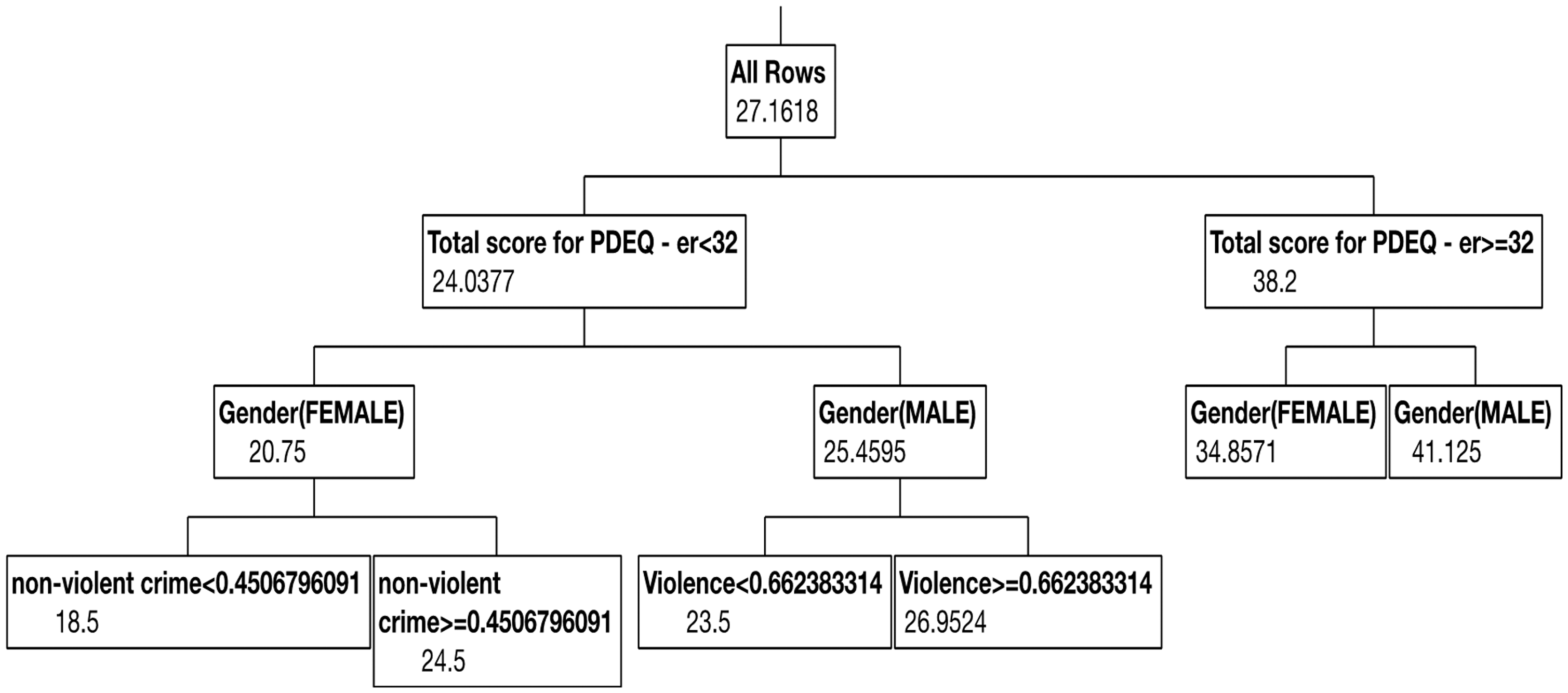

A significant limitation is that such methods can lead to overfitting, especially when the trees are “tall” where there are multiple extending branches. One way to prevent this is through the use of ensemble methods by repeatedly resampling from the data to build many trees (a forest) and then “vote,” or identify model branches across trees. A commonly utilized ensemble method is bootstrap aggregation (Bagging) ⁶⁸ in which the algorithm repeatedly selects random samples with replacement from the training set to fit trees and then averages predictions across all trees. This tends to reduce overfitting because each individual tree may be highly sensitive to noise in the training set while the model average across many trees is not, but only under the condition that individual trees are not highly correlated. Random forests extend this method by selecting random subsets of features to grow trees, often referred to as “feature bagging.” The purpose of this addition is to reduce correlations between trees.

Support Vector Machines

SVM classification algorithms attempt to build a classifier in multidimensional space (across many features or variables) that differentiates classes of individuals (e.g. cases vs. controls). ⁶⁹ SVMs achieve this by identifying a linear decision surface (e.g. a line in two-dimensional space) that separates classes with the largest distance (also called largest gap or margin) between objects that are at the borderline. While an infinite number of lines (or decision surfaces) can separate two classes, only one decision surface (support vector) exists that separates classes with the largest gap between borderline objects (see Figure 6). In this example, the support vector consists of two objects, one case and two controls (signified by yellow centers), together defining the line with the largest gap separating the two populations.

Figure 6.

Linear decision surface with widest margin. SVMs attempt to identify a line with the largest gap that separates out predetermined populations.

There are many instances where there is no way to linearly separate objects belonging to two classes. When no linear decision surface can be identified, SVMs “map” the data into higher dimensional space, termed feature space, where a separating linear decision surface can be identified. This act of mapping to higher dimensional space to identify a linear surface is known as the kernel trick. ⁷⁰ The kernel trick extends SVMs beyond linear classification to nonlinear classification. This framework makes SVMs particularly useful in contexts where a data set has hundreds or thousands of dimensions such as genes or proteins (see Figure 7). SVMs thus construct a hyperplane (or set of hyperplanes) in high-dimensional space that can be used for classification (or regression in the case of Support Vector Regression ⁷¹ where the score is a real number).

Figure 7.

Features that are not linearly separable being pulled into high-dimensional feature space. SVMs and other ML methods employ a technique known at the kernel trick whereby a linear decision surface is identifiable in situations where populations are not linearly separable by pulling data into higher dimensional space.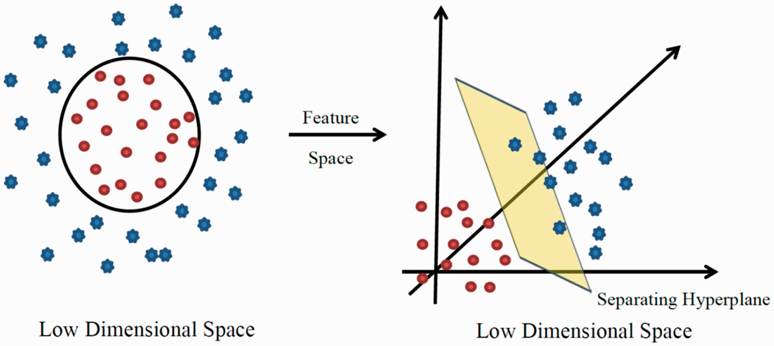

Regularized Regression

Another commonly utilized set of methods for both model fitting and feature selection is regularized regression. In many situations, it is not appropriate to assume that variables will relate to each other in a linear fashion as linear regression does. Regularized regression techniques, such as the least absolute shrinkage and selection operator (LASSO), ridge, and elastic net regression, are useful in such a context because they allow the data analyst to select the preferred level of model complexity from linear to highly nonlinear. Increasing the complexity of the model can lead to overfitting as such models can find odd patterns that are unique only to the data at hand. As such, regularized regression models include a regularization term which imposes a penalty as models increase in complexity, making model fit harder to achieve as the complexity of the model increases. The coefficients of variables that are not relevant to the model are shrunk to decrease their impact on the model (in the case of some models such as LASSO and elastic nets, they are shrunk to 0). This allows analysts to use these models for feature selection as the most relevant variables will be selected into the model and irrelevant ones will be discarded. One of the key benefits of regularized regression is that the models are highly interpretable because it is evident what variables are predictive as well as the degree of predictive accuracy.

Model Building and Validation

Often when building a model, data scientists will integrate multiple techniques to find and validate the best solution. Figure 8 provides a schematic of an approach that integrates multiple techniques: Figure 8(1): Individuals are clustered into one of the three groups (chronic, recovery, and resilient), using LGMM. Figure 8(2): A diverse set of variables of different types such as physiology, labs, and self-report assessments are prepared for modeling. Figure 8(3): The large set of variables is entered into an unsupervised feature selection algorithm (in this case, network models are employed for feature selection). Figure 8(4): A model is built that classifies individuals based on the remaining variables into the three groups (chronic, recovery, and resilient) based on knowledge of who is a member of each group. Next, a random subset of the original data that were not used to build the model is used to test it. Data sources are compiled (Figure 8(a)) and entered into the model that was built during the training step (Figure 8(b)). Figure 8(c): Based on the model, individuals are classified into groups. Figure 8(d): The accuracy of the model in correctly selecting individual’s membership in each group is calculated. In an ideal scenario, this model is then tested on a truly independent data set. This approach has been utilized for the prediction of PTSD following exposure to a potentially traumatic event^72–75 and is a common approach in other areas of medicine. ⁷⁶

Figure 8.

Machine learning classification workflow. The figure provides a schematic for a common approach to supervised ML prediction or classification. In this example, (1) we have individuals who are known to be part of one of the three populations (chronic, recovery, and resilient) along with (2) a set of variables of different types such as physiology, labs, and self-report assessments. (3) The large set of variables is entered into an unsupervised feature selection algorithm (in this case, network models are used for feature selection). (4) A model is built that classifies individuals based on the remaining variables into the three groups (chronic, recovery, and resilient) based on knowledge of who is a member of each group. This step is known as the training step, or model building. Next, the model is tested during the testing step. In this case, a random subset of the original data that was not used to build the model is used. (a) Data sources are compiled and (b) entered into the model that was built during the training step. (c) Based on the model, individuals are classified into groups. (d) The accuracy of the model in correctly selecting an individual’s membership in each group is calculated. In an ideal scenario, this model is then tested on a truly independent data set.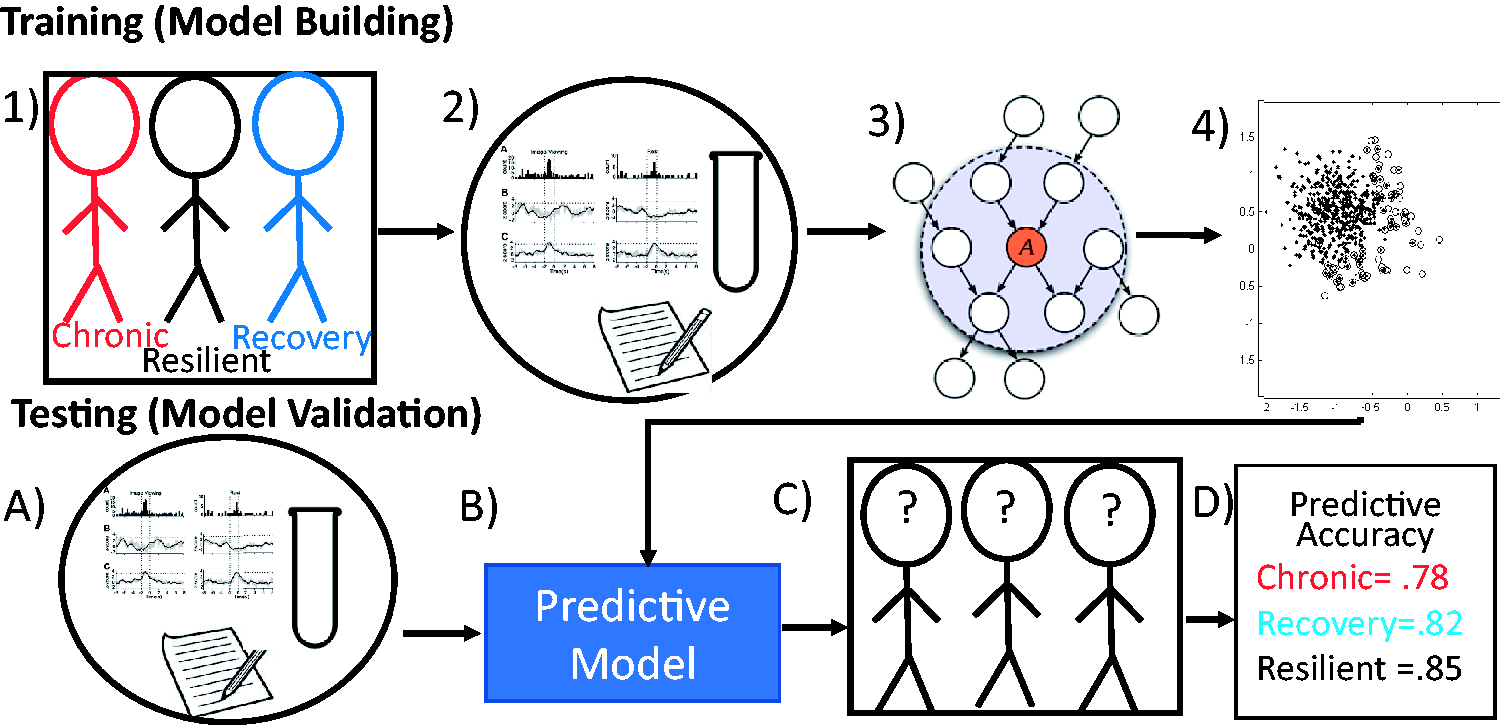

Reinforcement Learning

Dopamine (DA) is a neurotransmitter in the brain that initiates adrenalin during the activation of the stress response. DA rules motivational forces and psychomotor speed in the central nervous system. When a person is experiencing stress, the response system will be turned on, which will elevate stress hormones such as cortisol and reduce the level of serotonin and DA. Chronic stress or oversecretion of stress hormones may lead to imbalance of DA levels, and dysfunction of DA system (e.g. ventral tegmental area and nucleus accumbens) can potentially trigger various mental disorders, such as addiction, depression, distress, and anxiety. For instance, while high levels of DA cause drug “highs” or impulsivity (e.g. in addiction) and hyperactivity, low levels of DA may cause sluggishness and hypoactivity.

RL is an area of ML inspired by animal learning, behavioral psychology,^77,78 and dynamic programming methods. ⁷⁹ In ML, it is also formulated as a Markov decision process. The RL method is developed to resolve a temporal credit assignment problem, which provides a framework for modeling reward/punishment-driven adaptive behavior^80,81 and emotions. ⁸² Specifically, a subject or agent will learn to optimize a strategy to maximize the payoff or future reward through trial and error. The strategy is determined by its own value function V(s). The temporal difference learning is the most common model-free RL algorithm, ⁸³ which aims to learn a value function V(s) for the state [s] (the state can be a finite or infinite set) according to the one-step ahead prediction error (PE).

$$\text{V}({\text{s}}_{\text{t}})\leftarrow \text{V}({\text{s}}_{\text{t}})+\alpha [{\text{r}}_{\text{t}+1}+\gamma \text{V}({\text{s}}_{\text{t}+1})-\text{V}({\text{s}}_{\text{t}})]$$

where r_t denotes the reward or reinforcement signal at time t (which can be positive or negative or zero), 0 ≤ γ ≤ 1 is a discount factor for the reward, and 0 < α < 1 is a learning rate parameter. A positive PE ≡ [r_t+1 + γV(s_t+1) − V(s_t)] implies that the reward is greater than expected and therefore increasing the value V(s_t), whereas a negative PE leads to a decrease in V(s_t). Imagine an approach/avoidance task, the subject may need to learn a strategy (two actions: approach vs. avoid) depending on the cued stimulus in order to maximize the reward or avoid the punishment. In the simplest case, the value function can be represented as a look-up table, and each state–action pair is associated a value. Once the RL is accomplished, the agent will use the learned value function to guide behavior (i.e. action) in the environment (see Figure 9).

Figure 9.

Reinforcement learning schematic. Reinforcement learning (RL) can be formulated as a Markov decision process of an agent interacting with the environment in order to maximize the future reward. At each time step t, given the current state s_t (and current reward r_t), the agent needs to learn a strategy (i.e. the “value function”) that selects the optimal decision or action a_t. The action will have an impact on the environment that induces the next reward signal r_t+1 (which can be positive, negative, or zero) and also produces the next state s_t+1. The RL continues with a trial-and-error process until it learns an optimal or suboptimal strategy.

Stress has played an important role in DA-related pathophysiology. For instance, the relationship between stress and drug abuse can be modeled by dopaminergic/corticosteroid interactions. ⁸⁴ In a pioneering RL application to psychiatric disorders, addiction has been modeled as RL gone awry. ⁸⁵ Specifically, the effect of addictive drug is to produce a positive PE independent of the change in value function, making it impossible for the agent to learn a value function that will cancel out the drug-induced increase in PE. Specifically, the PE is replaced by

$$\text{PE}=\text{max}[\text{r}({\text{s}}_{\text{k}})+\gamma \text{V}({\text{s}}_{\text{k}})-\text{V}({\text{s}}_{\text{l}})+\text{D}({\text{s}}_{\text{k}}),\text{D}({\text{s}}_{\text{k}})]$$

where D(s_k) indicates a DA surge occurring on entry into state s_k. This modified equation will always produce a positive PE signal. Therefore, the values of states leading to a DA surge (D > 0) will approach infinity. While the DA neurons encode the PE, the addicted person’s brain will represent a specific “addicted” state s_k (e.g. drug, sex, or casino gambling) with an unusually high value function V(s_k).

More generally, different RL rules or rates can be adjusted according to either positive/negative reinforcement or positive/negative punishment to reflect the difference in rule sensitivity.

When confronting with aversive stimuli (stress factors), the agent can learn to inhibit a value function associated with the stress state s_k. The PE may be modified as

$$\text{PE}=\text{min}[\text{r}({\text{s}}_{\text{k}})+\gamma \text{V}({\text{s}}_{\text{k}})-\text{V}({\text{s}}_{\text{l}})+\text{D}({\text{s}}_{\text{k}}),\text{D}({\text{s}}_{\text{k}})]$$

where D(s_k) indicates a DA reduction occurring on entry into state s_k. In this case, D(s_k) can be a small positive value or even a negative value. In the long term, V(s_k) will converge to a negative value function independent of the positive or negative reinforcement.

Deep Learning

Deep learning is the application of multilayer (more than one hidden layer) artificial neural networks to learn complex representations of high-dimensional data patterns, such as images, videos, speech, and language. ⁸⁶ Deep learning may employ various network architectures, such as deep belief networks or recurrent neural networks. Learning algorithm can be supervised, semi-supervised, or unsupervised. Due to the large and deep network architecture, state-of-the-art optimization algorithms have been developed to tune the unknown high-dimensional (∼order of thousands or even tens of thousands) parameters. ⁸⁷ Research in the past decade has witnessed remarkable achievements in Artificial Intelligence(AI) in the era of BIG DATA.Due to powerful ability in representation and pattern discovery, we will expect a potential research application in computational psychiatry, where various heterogeneous sources of data (such as genes, behavior, family and medicine history, and neuroimaging) can be integrated within the ML framework to discover markers of risk and targets for treatment. The potential for deep learning will only be realized in mental health research as appropriate data sources become available. However, as large amounts of information on single individuals become available, the potential for discovery and characterization is enormous. Mental health researchers will soon be able to tap into massive sources of continuously recorded data that captures behavior in real time. Deep learning methods may quickly redefine behavioral constructs such as stress, ways of measuring them, and even the discovery of ways to manipulate such behavior for therapeutic purposes. A limitation of such models is that they are not straightforward to interpret and are very prone to overfitting.

Conclusion

ML-based methods provide a computational framework to conduct research in the RDoC era. These methods, with their ability to integrate multiple overlapping sources of data and define clinically relevant populations, have a great deal to offer stress pathology and stress resilience research. The promise of this nascent field will only be truly realized as sources of data become available that are of the size and scope to truly build and validate such complex models. Because of the power of these tools to find solutions, there is a heightened need for caution, rigor, and an understanding of the underlying principles and limitations of such approaches. We hope that this review has provided information about diverse methods in a manner that encourage researchers interested in stress pathology to begin to think about how they can instantiate computational models that match the complexity of their hypotheses.