
Abstract
Probabilities or confidence values produced by artificial intelligence (AI) and machine learning (ML) models often do not reflect their true accuracy, with some models being under or overconfident in their predictions. For example, if a model is 80% sure of an outcome, is it correct 80% of the time? Probability calibration metrics measure the discrepancy between confidence and accuracy, providing an independent assessment of model calibration performance that complements traditional accuracy metrics. Understanding calibration is important when the outputs of multiple systems are combined, to avoid overconfident subsystems dominating the output. Such awareness also underpins assurance in safety or business-critical contexts and builds user trust in models. This article provides a comprehensive review of probability calibration metrics for classifier models, organizing them according to multiple groupings to highlight their relationships. We identify 94 metrics, and group them into four main families: point-based, bin-based, kernel or curve-based, and cumulative. For each metric, we catalog properties of interest and provide equations in a unified notation, facilitating implementation and comparison by future researchers. Finally, we provide recommendations for which metrics should be used in different situations.
1. Introduction
Artificial intelligence (AI) and machine learning (ML) models have seen widespread adoption in recent years. When such models are used in safety or business-critical applications, it is vital to be able to understand and assure their behavior. Models generate predictions accompanied by confidence scores or probabilities, which are considered calibrated when they accurately reflect the proportion of correct classification decisions. However, confidence scores are not always representative of true probabilities. Assessing model calibration, particularly under any operational conditions that differ from training, requires a robust measure of calibration quality.
The publication of Guo et al. (2017), which highlighted examples of miscalibration in deep neural networks, sparked an intense interest in the concept of calibration and metrics to measure it. This surge in attention has led to numerous publications over the last few years, with approximately ten new metrics being defined and proposed every year since then, and many papers discussing their merits or application. However, as Flach and Song (2020) witheringly put it in their conclusion, “contrary what recent machine learning literature may lead you to believe, calibration research predates machine learning and has been studied for three-quarters of a century.” Thus, there is a large body of work from which to draw on. Silva Filho et al. (2023) were motivated to write a survey on assessing and improving classifier calibration as “the literature on post-hoc classifier calibration in ML is now sufficiently rich that it is no longer straightforward to obtain or maintain a good overview of the area.” This lack of understanding has caused an impediment to research, requiring scientists to examine numerous papers to find relevant information. Indeed, despite the valuable survey of Silva Filho et al. (2023), it only covers a small subset of available metrics.
This article presents a comprehensive review of classifier probability calibration metrics. The aim of the review is to serve as a useful reference for researchers attempting to understand the landscape of such metrics. Contributions of the article are as follows: A wide-ranging survey of classifier probability calibration metrics for models with a discrete output is provided. This review addresses a gap in the literature for which there is a high demand. Maier-Hein et al. (2024) in their major review of general classifier metrics, originally intended to omit the class of calibration metrics but the decision was reversed due to high demand expressed through crowdsourced feedback. Nevertheless, that review only covers a small fraction of the calibration metrics described in the present article. Metrics are organized according to several novel categorizations to understand the relationships between them. The main categorization is the four families of point-based, bin-based, kernel or fitted-curve, and cumulative metrics. Each family has advantages and disadvantages, as do individual metrics within families. These are described in detail in the article. This article represents the most comprehensive survey of probability calibration metrics to date, providing descriptions of significantly more metrics than those in the overlapping lists provided by other authors. The five most similar reviews are by Flach and Song (2020; who describe seven metrics), Hagopian et al. (2023; 13 metrics), Silva Filho et al. (2023; nine metrics), Maier-Hein et al. (2024; eight metrics), and Tao et al. (2024a; 11 metrics). Between them, these five reviews discuss 26 metrics, whereas the present article analyzes 94 metrics. Where relevant, equations are provided with a unified notation to facilitate implementation and comparison by future researchers. Original papers that first describe metrics use a wide variety of different notations, making comparisons difficult. Metrics that were previously treated in isolation are brought together and conceptual relationships are highlighted. Several authors have independently invented the same metric but given them a different name. This review treats such metrics as a single entry and consolidates the separate analysis provided by the original authors. Some metrics are special cases of others but have not previously been associated. These connections are noted along with integrated discussions. Other metrics that are nominally from different families, but have conceptual similarity, are discussed together, enabling cross-fertilization of ideas between different research groups. Finally, we recommend specific metrics for general, multiclass, and local calibration scenarios.
The remainder of this article is organized as follows. Section 2 introduces key concepts relating to calibration metrics and defines major notations used in this article. Sections 3–6 respectively describe metrics in the point-based, bin-based, kernel or fitted-curve, and cumulative families. A dendrogram showing the hierarchy of families and subfamilies is shown in Figure 1. Conclusions and recommendations are given in Section 7. Appendix A describes lesser-used metrics. Appendix B includes further discussion on skill scores, bootstrapping and consistency sampling, and consistency calibration. Appendix C contains a comprehensive list of symbols and their basic definition. Finally, Appendix D contains a table that summarizes the main pros and cons of each metric and other information, such as the range of attainable values and alternative names for the same metric.

Hierarchy of probability calibration metric families and subfamilies.
2. Calibration Metric Concepts
2.1. Notation
The literature on probability calibration metrics is inconsistent in terminology and notation. We describe techniques in a unified way, rather than using original symbolizations. We start by defining the problem of interest to be assigning a piece of data or “datapoint” to one of K classes. The data could be a feature vector, image, signal, time series, or any other collection of information. Each datapoint, while potentially representing multiple numbers, is treated here as a single, possibly multidimensional, entity. Each datapoint i has an associated true label
For each datapoint, the model produces a predicted probability or confidence
A more comprehensive list of symbols used in this article and their basic definition is given in Table 3 in Appendix C. Each term is described in more detail where it first appears in the article.
2.2. Calibration Curve and Reliability Diagram
An ideally calibrated classifier outputs confidence scores or predicted probabilities equal to its accuracy, conditional on the score. The term “accuracy” is also named in various sources as “actual positive rate,” “fraction of positives,” “empirical probability,” or “observed relative frequency.” In practice, the accuracy for a particular confidence value can be higher or lower than that confidence. The actual accuracy as a function of confidence for a particular class is known as the calibration curve. An example theoretical nonperfect calibration curve is illustrated in Figure 2, along with the ideal calibration line. In this example, the classifier is overconfident in the target class—the achieved accuracy is lower than the model's confidence. In binary classification, the calibration curve for Class 1 contains all the information necessary to understand the model's calibration, as the curve for Class 0 is its complement. Multiclass models are more complex, as discussed in Section 2.3.
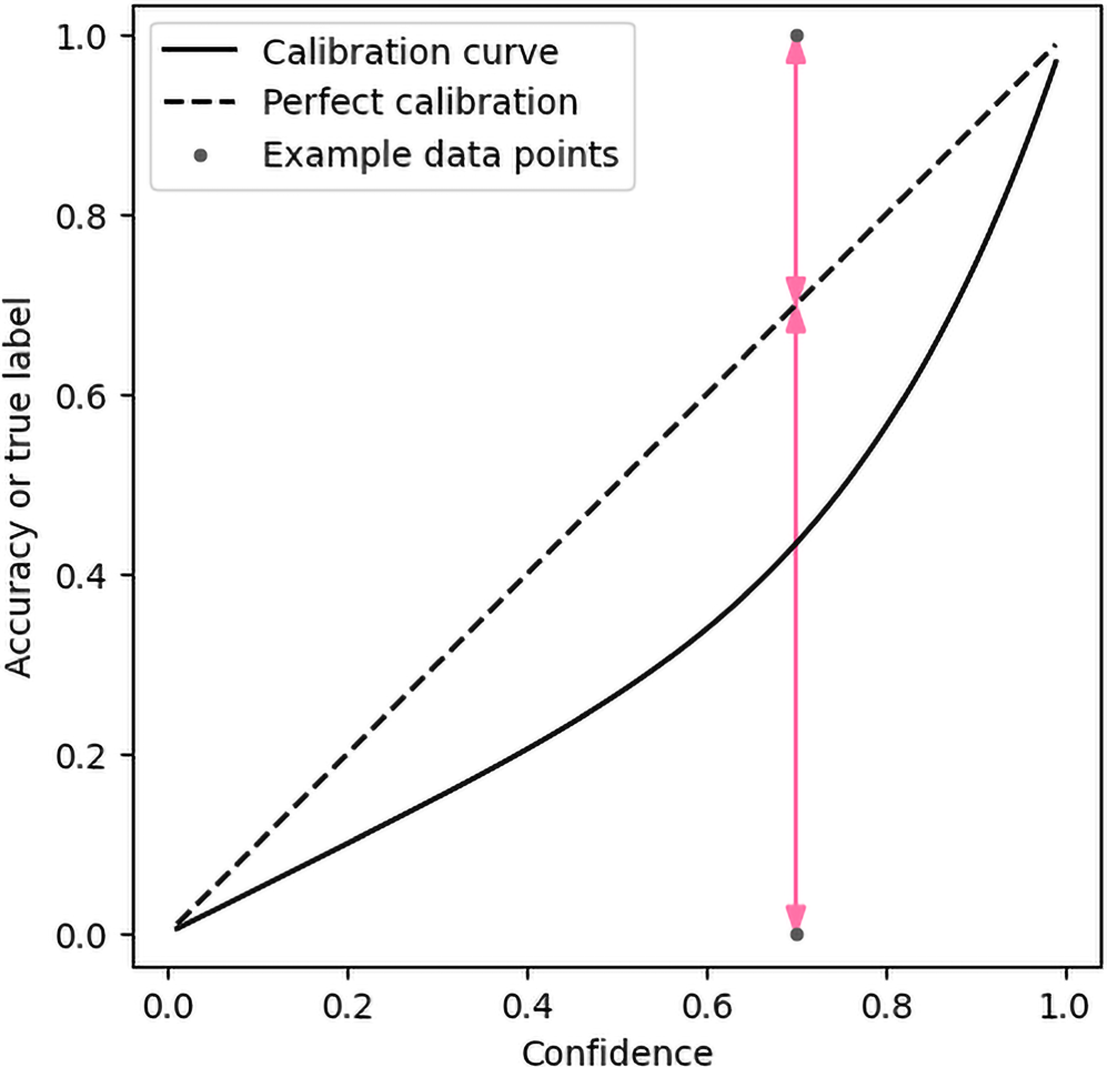
Theoretical calibration curve with two example datapoints having the same confidence, but different true labels. The red arrows indicate the calibration errors for those individual datapoints. The curve represents an overconfident classifier.
For a single datapoint, the classifier is either correct or incorrect, and the model can only perfectly be calibrated if the confidence is zero or unity. For other confidence values, there is inevitably some calibration error. Figure 2 demonstrates this for two example datapoints with the same confidence value of 0.7 for Class 1. The true label is zero for one datapoint and the error for that datapoint is 0.7, indicated by the lower red arrow. The true label for the other datapoint is unity, and the error for that datapoint is 0.3, indicated by the higher red arrow.
Although perfect calibration for a single datapoint is impossible without perfect accuracy, a classifier with nonperfect accuracy over a set of datapoints may still be well calibrated. For example, if 10 datapoints all have a confidence of 0.7 and seven out of those 10 are classified correctly, then this classifier is perfectly calibrated for the dataset. In practice, not all confidence values output by a model are expected to be identical, so confidence values are often grouped into nonoverlapping bins and the accuracy of datapoints in each bin is analyzed. The visual representation of this information is known as a reliability diagram, curve, or plot. This is frequently shown as a bar chart, see Guo et al. (2017) for example. However, line plots facilitate better visual inspection of the data because they show trends over the underlying continuous confidence variable. Some works place markers at the center of each bin on the horizontal confidence axis. However, if the data are not uniformly distributed throughout the bin this can give misleading results. Therefore, it is better to place markers at the mean confidence for each bin (Silva Filho et al., 2023). Vasilev and D'yakonov (2023) distinguish between the bar chart representation being called the reliability diagram and the line representation being called the reliability plot.
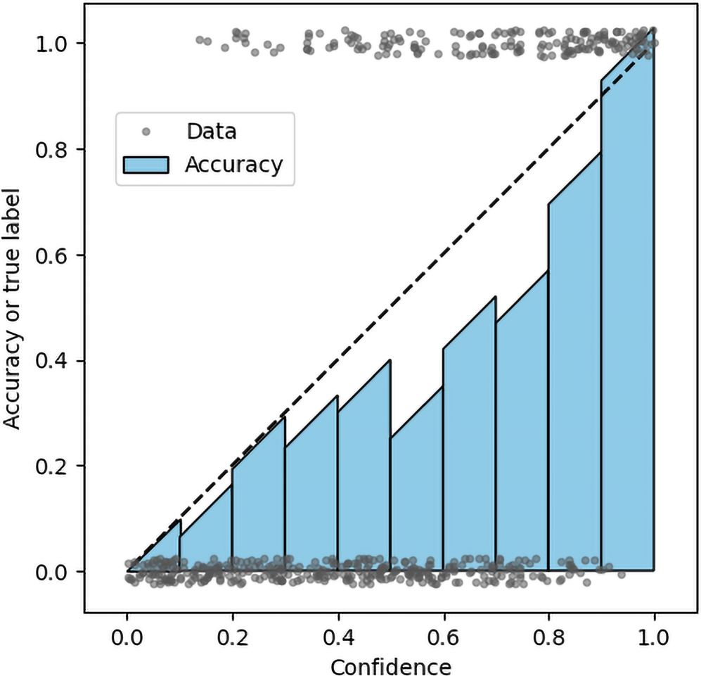
An example reliability plot is shown in Figure 3 as a solid line, and additional information is included. The dataset used to compute this diagram was generated as 500 random samples, with confidence values and true labels determined based on the true calibration curve in Figure 2. In Figure 3, true labels are jittered by ±0.025 for improved visualization. The markers on the reliability curve show the mean achieved accuracy in 10 equal-width bins, and the error bars represent the standard error of those estimates. The standard error is greater for confidence values near 0.5 than zero or unity and is in general greater when there are fewer datapoints, although this effect is not apparent for this example dataset. The measured reliability curve is approximately the same shape as the true calibration curve. The same information is shown in Figure 4 using the slightly more common bar chart representation.

Reliability line plot for 500 labeled datapoints, with ten bins. The plot shows that, for a finite dataset, empirical accuracy does not always increase with confidence.

Reliability bar chart for 500 labeled datapoints, with 10 bins. The chart emphasizes EW of the bins.
Most binary calibration metrics measure some aspect of the data visible in Figures 2, 3, or 4, whether this is the location of the datapoints, or the degree to which the calibration curve, as estimated via binning or other means, deviates from the identity line.
2.3. Multiclass Aspects
Most work on probability calibration metrics relates to binary classifiers. However, multiclass versions also exist. There are three ways to define calibration for multiple classes (Silva Filho et al., 2023):
Vaicenavicius et al. (2019) give theoretical examples where a multiclass classifier is either top-label calibrated or class-wise calibrated, but not fully multiclass calibrated. Lack of full multiclass calibration could be important in safety critical applications, especially where the action taken should depend not only on the most likely outcome, but also the probabilities of other less-likely outcomes, which may have severe negative consequences.
Multiclass problems are often decomposed into binary subproblems whose outputs are aggregated to give an overall multiclass score (Kull & Flach, 2014). The most common decompositions are OVR or comprehensive pairwise. The advantage of such decompositions is that binary classification theory and practice, including probability calibration, can be applied to subproblems without the complication of multiclass issues. Furthermore, some classifiers are inherently designed only to work with binary problems. Decomposition allows these classifiers to be applied in a multiclass setting without further modification. The disadvantage of OVR decompositions is that only class-wise calibration can be measured, not full multiclass calibration.
2.4. Other Observations on Calibration
Numerous studies have empirically shown that classifiers often exhibit overconfidence. The usual explanation given is that the models are large enough to memorize training data and maximize confidence. However, Bai et al. (2021) show that certain classifiers are inherently overconfident, even when the dataset is large and the number of model parameters is small. Specifically, this applies to logistic regression and other classifiers where the activation function is symmetric and concave in the positive half. Munir et al. (2022) state that rectified linear unit activation functions, widely used in modern deep neural nets, and similar piece-wise linear functions, are a core reason behind overconfident predictions in test data far away from the training data. Minderer et al. (2021) show that model structure is more important than model size in understanding probability calibration, and that recent models, especially those not using convolutions, are in fact among the best calibrated.
The metrics described in this article serve as absolute measures of model calibration. Recalibration techniques attempt to improve the correctness of model confidence values by post processing. The aim of such techniques is to invert the effect of the model calibration curve so that the overall process produces the identity function. In practice, these techniques are not perfect, but their “calibration gain” can be defined, which is the improvement in calibration error (by any metric) when the technique is applied (Zhang et al., 2020).
2.5. Scope of Article
A systematic and comprehensive review of classifier probability calibration metrics was conducted as follows. First, Google Scholar was used to generate a long list of the top 100 papers that included the words “probability,” “calibration,” and “metric,” starting from the year of the seminal paper by Guo et al. (2017) that spurred recent widespread interest in probability calibration. From this long list, papers that did not describe a new metric or compare existing metrics, were removed, leaving a short list. Metrics that can be used as classifier probability calibration metrics, even if they were originally designed for another purpose, such as a loss function, were defined as in scope. Forward and backward citation searching, seeded from this short list, was performed to cover any gaps from the initial search. The result of this process was a list of papers that collectively comprehensively describe classifier probability calibration metrics. The metrics were then analyzed, grouped into families, and explained in this article. We include new insights into relationships and properties of these metrics.
Although this review focuses on classifiers, object detection models also produce probabilistic outputs and pose related calibration challenges. Whereas as a classifier only considers the discrete label of a piece of data, an object detector also provides object size and location co-ordinates, often within an image. Although object detector confidence scores can be assessed based only on labels of associated ground-truth objects, the additional degrees of freedom allow a more nuanced form of assessment. Analysis of object detection is out of scope for this article. Example probability calibration metrics specific to object detection are discussed by Neumann et al. (2018), Küppers et al. (2020), Conde et al. (2023), Oksuz et al. (2023), Popordanoska et al. (2024), and Kuzucu et al. (2025).
This survey concentrates on the assessment of model probabilities rather than methods to improve calibration. Reviews of such methods are covered well by Flach and Song (2020) and Silva Filho et al. (2023). The present article focuses on reporting practical mathematical definitions of metrics, their properties, why they might be used, and a summary of existing performance analyses. Experiments that perform numerical comparisons of small subsets of metrics have been conducted elsewhere—see Widmann et al. (2019), Zhang et al. (2020), Gruber and Buettner (2022), Roelofs et al. (2022), Matsubara et al. (2023), Peng et al. (2023), or Kängsepp et al. (2025), for example. New experiments to provide a comprehensive comparison would be a significant undertaking requiring thousands of hours of compute time (Kängsepp et al., 2025) and are not included here for space reasons. A full description of the in-scope probability calibration metrics, arranged by family, now follows.
3. Point-Based Metrics
3.1. Introduction to Point-Based Metrics
Point-based metrics compute a score for each datapoint
3.2. Proper Scores
Proper scoring rules are point-based evaluation measures for probability estimates that avoid the need to put confidence scores into bins (Silva Filho et al., 2023). Following Bröcker (2009), a scoring rule

By convention, low scores indicate good predictions. A score is “proper” if the divergence
Strictly proper scores can be decomposed into three terms: reliability, resolution, and uncertainty, which facilitates interpretation of the score (Bröcker, 2009):

Reliability is a measure of the degree to which predictions differ from the actual sample relative frequencies (Murphy, 1973), with lower values being good. In early works, reliability was referred to as validity, but it is often now known as calibration loss (Silva Filho et al., 2023). As an illustrative example, if a classifier only produces confidence values of exactly 90% or 70%, and is respectively correct 90% or 70% of the time for those specific values, then the classifier is “reliable” and has a reliability value of zero.
Resolution quantifies how much the sample proportions for each unique predicted probability differ from the overall sample proportions for the whole dataset (Murphy, 1973), with higher values being better. For example, consider a binary dataset where 50% of the datapoints belong to either class. A classifier that always gives a confidence of 50% and chooses randomly between the two classes would have an accuracy of 50% and be well-calibrated globally, but not particularly useful. This classifier has zero resolution. An alternative, reliable classifier that randomly gives confidence scores of 80% or 20% half the time to Class 1, has a better, nonzero resolution, despite also having an accuracy of only 50%. Resolution is also called sharpness (Bröcker, 2009).
Uncertainty is the score that would be achieved by replacing confidence values with the proportions of the actual samples (Murphy, 1973), with lower being better. Thus, this term is inherent to the data and does not relate to the classifier. For example, if 80% of the datapoints are from one class, a theoretical classifier that always gives a confidence value of 80%, would achieve a score equal to the uncertainty value. If all datapoints are from one class, the uncertainty is zero. In a binary classifier, the uncertainty is highest when half of the datapoints belong to each class.
The three-term decomposition of scores is only useful when more than one datapoint has the same predicted probability vector. This may be the case for human forecasters that are prone to specifying probabilities on a discrete scale (10%, 20%, etc.). However, algorithms specify probabilities on a continuous scale from zero to unity and it is unlikely that many predicted probability vectors will have the same exact value. When all probabilities are different, the resolution and uncertainty terms cancel out, and the reliability is the same as the overall score. Thus, the decomposition has less utility in modern algorithmic contexts than traditional human prediction analysis.
An alternative decomposition considers proper scores as a sum of two components: epistemic loss, due to the model not being optimal, and an irreducible or aleatoric loss, which is the loss of the theoretically optimal model, due to randomness in the data (Silva Filho et al., 2023). This decomposition helps focus analysis on parts of the problem that are in control of model designers. Other decompositions are also available (Popordanoska, 2025).
Silva Filho et al. (2023) recommend that classifiers should be trained using a proper scoring rule as loss function rather than nonproper functions. This is because the resulting models are likely to produce better probabilities, since probability refinement and calibration would be encouraged during training.
3.3. Brier Score
The Brier score (BS) is one of the earliest and best-known calibration metrics. It is a common way of measuring how much the accuracy of a model diverges from its confidence, with lower scores meaning the model is well calibrated. The BS is also called mean square error (MSE) (Flach, 2019) or the quadratic score (Gneiting & Raftery, 2007). The BS can be calculated by equation (3).

The score can be thought of as the mean of the squares of the arrowed data-point calibration-error line distances in Figure 2. Initially developed for weather forecasting, the BS is now widely used as a general measure of risk prediction. It has advantages that it is easily calculated and interpreted and is a strictly proper score. The original definition of BS for binary classifiers is in the range
The square root Brier score (RBS) is a robust estimator and upper bound of the canonical calibration error. RBS is compared to bin, kernel, and cumulative metrics in Gruber and Buettner (2022). Of the metrics tested, only RBS and the cumulative Kolmogorov–Smirnoff (KS) metric are consistent in value with respect to data size—a desirable property.
3.4. Logarithmic Metrics
Negative log likelihood (NLL), also called binary cross-entropy, ignorance (Bröcker, 2009), logarithmic score or predictive deviance (Gneiting & Raftery, 2007), logistic loss (for binary problems), or multinomial logistic loss (for multiclass problems) is calculated by the equation:

The NLL takes on any nonnegative value and is strictly proper (Tödter & Ahrens, 2012). When NLL is small, the model is well-calibrated. Like the BS, NLL is easy to compute but conflates accuracy and calibration (Gupta et al., 2021). One issue with NLL is that if the confidence is zero for the correct label for any datapoint, the NLL evaluates to infinity. This reflects the fact that a good prediction system should never assign zero probability to possible events (Tödter & Ahrens, 2012). If the confidence is a small value instead of zero, the NLL can still be very large. Thus, the metric severely penalizes highly unlikely predictions, which may be an indicator of lack of calibration. However, this means that single datapoints can have a large effect on the overall metric value, which is an undesirable property (Gneiting & Raftery, 2007). Considering that some datasets have "label noise" where the supposed ground truth labels are incorrect for a small proportion of datapoints, this property of the metric has potential to cause major issues.
Focal loss (FL) is a modified version of NLL designed to focus on hard-to-classify examples (Lin et al., 2017). FL is defined as:

When
Sumler et al. (2025) describe a general metric to measure the consistency of continuous or discrete probabilistic algorithms, including multitarget trackers, classifiers, multihypothesis trackers, and particle filters. They derive a simplified version of this metric when applied to binary classifiers and call it the entropic calibration difference (ECD). This is defined as:

ECD is a signed metric—it can take on any value on the real line. When positive, the classifier is overconfident. When negative, the classifier is underconfident. When zero, the classifier is perfectly calibrated. The signed nature of the metric is an advantage compared to other metrics that only give information on whether a classifier is calibrated without the direction of miscalibration. The absolute value of ECD is a proper scoring rule.
3.5. Global Metrics
Global metrics compute the mean confidence of all datapoints and compare this to the mean accuracy. The two numbers are expected to match for a calibrated system. This type of metric is included as a point based metric due to its use of simple sums over the datapoints. However, global metrics are also a bin-based metric with a single bin for the entire dataset. Individual metrics vary in how they compare the global sums. Due to the use of aggregate statistics, global metrics are not proper.
The global squared bias (GSB) is defined by Galbraith and Van Norden (2011) as:

The GSB is a measure of the match between the unconditional mean predicted probability and the unconditional mean probability of the outcome. The metric, as defined in equation (7), takes on values between zero and unity. However, when comparing GSB with the old definition of BS, many authors omit the
Another metric like the GSB is the multiclass difference of confidence and accuracy (MDCA). It is defined by Hebbalaguppe et al. (2022) as:
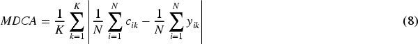
MDCA was designed to be used as an additional loss term for minibatches of data in neural net training to encourage calibrated models. However, it can be used to assess calibration of the whole dataset. The metric is differentiable, which allows it to be used as part of gradient descent algorithms. The metric is equivalent to the ECE (see Section 4.2) with a single bin for all probabilities.
Another global metric for binary problems is the ratio of the expected to observed (EO) number of datapoints in the target class:

The metric takes on nonnegative values on the real line. If
3.6. Normalized Square Metrics
The Dawid–Sebastiani score (DSS) is a metric for models that output general probabilistic predictions, using the first two statistical moments of the predictive distribution. DSS is defined by Moore et al. (2022) as:

In (10),
The normalized squared error score (NSES) is defined by Moore et al. (2022) as:

NSES takes on any nonnegative value. The metric is like the DSS but omits the logarithmic term. However, unlike DSS, NSES is not proper. Despite its impropriety, NSES is considered by Moore et al. (2022) to have valuable diagnostic properties, as it can be used to distinguish overconfidence
3.7. P-Norm Metrics and Variants
The pointwise
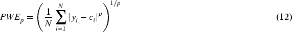
When
De Leeuw et al. (2009) define a modified version of

This is similar to a pseudo Huber loss (Barron, 2019); see Appendix A.8 for the standard Huber loss. For small errors L1eps acts like the
4. Bin-Based Metrics
4.1. Introduction to Bin-Based Metrics
Point-based metrics such as the BS have been used to measure calibration for several decades. However, one issue with such metrics is that it is usually impossible for a classifier to achieve a perfect score under such systems. This is because if any confidence other than pure certainty is predicted for a particular datapoint, there will be a difference between the confidence and the label for the correct class, which is zero or unity by definition. Thus, the only way for a classifier to be assessed to have perfect calibration, is if it only ever assigns a confidence of 100% to the correct class and is always correct. This is impractical for any real dataset.
Bin-based metrics group datapoints with similar confidence values. The proportion of correct classification in each bin can then be compared to the mean confidence of the bin, or some other single value representative of all the datapoints in the bin. This allows imperfect, but well calibrated, classifiers to achieve a good calibration score. An illustration of binned data is shown in Figure 4. Conceptually, bin-based metrics are based on the difference between the binned accuracy and perfect calibration lines.
The remainder of this section describes several bin-based metrics and their advantages and disadvantages. One general disadvantage is that a small change in confidence value of one datapoint can cause it to be assigned to an adjacent bin, resulting in a discrete jump in metric value, which may be undesirable. The following notation specific to binned metrics is used. The number of bins is B, the number of datapoints in bin b is
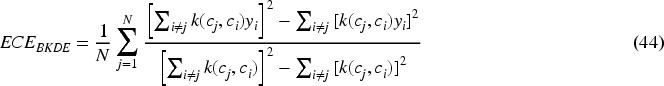
4.2. Expected Calibration Error
ECE is a widely used metric for quantifying the miscalibration of probabilistic classifiers, where lower values indicate better calibration (Guo et al., 2017). Some authors call ECE “empirical” or “estimated” instead of “expected,” as it is not a true expectation (Silva Filho et al., 2023). The binary-ECE is calculated via the formula:

The standard form of ECE uses equal width (EW) bins so it is sometimes named ECE-EW (Roelofs et al., 2022). ECE is also called the mean absolute calibration error (Lee et al., 2023). ECE is easy to compute and visualize—it is the absolute area between estimated and perfect calibration bars—see Figure 4.
Despite widespread use, ECE has several disadvantages. First, it is trivially possible to obtain perfect ECE by randomly estimating examples according to the label distribution (Liu et al., 2020). For example, in binary classification, if 60% of data examples are from Class 1, then assigning a confidence of 60% to all items, regardless of input features, will produce a perfectly calibrated classifier, according to ECE, but one with poor accuracy.
Second, some fixed bins may have very few or no datapoints. Thus, the calibration error for those bins either cannot be computed or has a very high variance, which is reflected in the overall ECE. Datapoint sparsity for some bins is demonstrated by Guo et al. (2017), who provide an example histogram of the number of samples in each bin for an image classifier. Low confidence bins have very few samples, and the lowest two bins have no samples at all.
Third, in multiclass problems, standard ECE is computed for the highest probability class only. In this case, it is known as top-label classification error (Kumar et al., 2019) or confidence-ECE (Silva Filho et al., 2023). However, it may be important to distinguish between second, third, or lower ranking classes when the assessment from the classifier under test is being combined with other information (Widmann et al., 2019).
Fourth, ECE conflates calibration and sharpness when a model is highly accurate (Nixon et al., 2019). Sharpness is the desire for models to predict with high confidence. This conflation issue is related to the two previous ones. Since only top-label confidence is analyzed, confidence values are naturally concentrated toward unity. As ECE places a low weight on sparsely populated bins with low confidence, the metric relies primarily on high confidence bins. For these high confidence values, an accurate classifier has tall bin heights that are near the line of perfect calibration in the reliability diagram. Thus, the accurate classifier naturally has a lower ECE than if confidence values were more uniformly spread.
Fifth, ECE depends on the scale of probabilities. If many probabilities are small (e.g., 0.001), this results in a small ECE even if the achieved accuracy is also small but is many factors times the confidence (e.g., 0.01, a factor of 10 difference; Matsubara et al., 2023).
Sixth, ECE is a highly discontinuous function of classifier confidence values due to its fixed width bins. This makes it a difficult metric to use in gradient-based optimization schemes (Kumar et al., 2018), and a small change to a single confidence value could have a large effect on the overall ECE.
Seventh, for a model with a certain fixed calibration performance, the value of ECE decreases as the number of datapoints used to compute it increases (Gruber & Buettner, 2022). This complicates comparisons across datasets of different sizes.
Due to these shortcomings, several variations of ECE have been proposed. These are described in subsequent sections. However, we first describe some general definitions for binary and multiclass classifiers that aid discussion of such metrics.
4.3. Mean Calibration Error
The

This general definition incorporates several well-known specific metrics. Kumar et al. (2019) state that the most common value is
4.4. Binned Multiclass Calibration Error
For confidence bin b and class k, let the class-specific mean confidence and true proportion of data labels be denoted by

If
For full multiclass-ECE, probability vectors could in theory be binned in simplex space. The difference between the mean probability vector and the vector of class proportions in each bin could then be computed. However, most bins would likely be empty or have very few datapoints (Silva Filho et al., 2023). This can be seen as follows. If each dimension (class) is subdivided into G grid values, then the total number of bins is
4.5. Variants of ECE
Several minor variants to ECE have been proposed. Rather than using equal-width confidence bins, adaptive calibration error (ACE) by Nixon et al. (2019) uses bins based on fixed percentiles of confidence scores in the test dataset, so that each bin has the same number of datapoints. ACE is computed class-wise over all classes for multiclass problems, like the static calibration error. ACE is also called equal-mass (EM) ECE, or ECE-EM (Roelofs et al., 2022). Estimators with bins of equal mass have lower bias than estimators with bins of EW (Roelofs et al., 2022). EW and EM methods of binning are also referred to as width binning and frequency or quantile binning, respectively (Silva Filho et al., 2023). A disadvantage of ECE-EM is that some parts of the confidence space may have wide bins, preventing the ability to model variation in accuracy in those regions. The equal-area ECE (ECE-EA), or “equiareal ECE,” has bins with approximately equal area, providing a middle ground between ECE-EM and ECE-EW (Röchner et al., 2024). Thresholded ACE (TACE) uses frequency binning but only includes datapoints with a confidence value above a certain threshold. The logic behind this is that in situations with many classes, many class probabilities are low, and this washes out the calibration score. A threshold of 0.01 is used by Nixon et al. (2019). When only the top k confidence datapoints are selected, the method is called ECE@k (Guilbert et al., 2024). ACE and TACE are both relatively robust to label noise, a situation where lower-rank predictions are more important (Nixon et al., 2019). Nixon et al. recommend that ACE generally be used in favor of other metrics or standard ECE. However, if the number of classes exceeds 100, they recommend TACE. Nevertheless, ACE and TACE only measure class-wise calibration, not full multiclass calibration.
Calibration can also be assessed by the area between the reliability plot and the ideal line, as seen in Figure 3. This is known as the area between curves (ABC), or the integrated calibration error, in Hagopian et al. (2023). The total absolute area is the standard ECE when the curve is constructed as a binned estimate. It is also possible to provide separate reports of the area above the curve, representing underconfidence in some regions, and below the curve, representing overconfidence in other regions (Hagopian et al., 2023). Reporting above and below areas is a useful decomposition of ECE (which is the sum of the two areas) to better understand under and overconfidence. However, the need to analyze two variables makes above/below ABC harder to use when assessing multiple recalibration algorithms automatically.
MCE is like ECE but instead of measuring an average of the calibration errors, MCE measures the largest calibration error. This is useful when it is important for a model to be extremely well calibrated across a range of confidence values. MCE is calculated by:

MCE can lead to unintuitive results when there is wide variance in calibration between histogram bins, which is more likely to happen when the test set is small. In these situations, the metric is highly sensitive to the placement of bins (Silva Filho et al., 2023). MCE may be most suitable for safety-critical applications, where it is important to understand the worst-case calibration at any confidence level. MCE is also called the
Region-balanced ECE (RBECE) is defined by Dawkins and Nejadgholi (2022) as:

In (18),
The monotonic sweep calibration error ECE-SWEEP chooses the largest number of bins for which the bin heights, as computed by standard ECE, are monotonic. When tested on data, it is found that the optimal bin count grows with sample size (Roelofs et al., 2022). An efficient implementation of the sweep method for choosing the number of bins is the bin count search (BCS) method—see Section 4.12 for its application as part of a debiased metric. ECE-SWEEP has a lower bias than several other metrics, including standard ECE—see Section 4.13. As with many other metrics, the disadvantage of ECE-SWEEP is that its standard definition is for binary rather than multiclass classification. However, measurement of class-wise calibration can be achieved through an OVR strategy.
4.6. Partially Binned Metrics
Distance from calibration error (DCE) is introduced as a theoretical measure by Błasiok et al. (2023). Angelopoulos et al. (2025) provide a bin-based empirical estimate of DCE with bins of EW for binary classifiers. Let the confidence

This metric operates on labels as points but confidences as bins—a partial binning strategy. The DCE estimate in equation (19) is shown by Angelopoulos et al. (2025) to be a tight upper bound on the true DCE for a sensible choice of B as the sample size N grows.
The Sanders-modified BS (SMBS), or Murphy's BS, is a partially binned version of the BS (Hagopian et al., 2023). Like DCE, SMBS uses binning to estimate aggregate confidence values in a bin while keeping the labels as individual points. A subtle difference between DCE and SMBS is that DCE uses max aggregation, but SMBS uses mean aggregation to obtain

For real datasets, the difference between SMBS and BS is small (Hagopian et al., 2023). Apart from the difference in aggregation strategy, SMBS is the
Label-binned calibration error (ECE-LB) uses binning to estimate true proportions of labels

ECE-LB is at least as large as standard ECE. It has the advantage over many other binned metrics that it considers the variation of confidence values in each bin rather than relying only on their mean. ECE-LB is named probability deviation error in Torabian and Urner (2024), where it is shown to have a lower bias than ECE.
4.7. Fit-on-the-Test ECE
The Fit-on-the-test (FOTT) calibration error is a metric subfamily that compares a calibration map

Kängsepp et al. (2025) define a binning scheme where, instead of assuming constant probabilities based on the mean within a bin, bin probabilities may be non-continuous piecewise linear functions of the input confidence. This binning scheme defines
Tilted-roof reliability diagram for 500 labeled datapoints, with 10 bins. The diagram facilitates comparison of bar heights with the perfect calibration line.
The number of bins used with ECE can be selected through cross-validation by optimizing the ECE-FOTT loss. The optimum number of bins for a calibration task containing 5,000 datapoints was 14. It is interesting that this is in the range of 10–20 bins that are usually arbitrarily used in standard ECE calculations. This suggests the number of bins typically used is sensible. However, according to Popordanoska (2025), there is no optimal default number of bins, since every scenario has its own bias-variance tradeoff.
4.8. Multipartition Metrics
The interval calibration error (ICE) is a theoretical metric that averages the ECE over all possible bin widths and locations. In practice, it cannot be computed directly, as the number of possibilities is huge for large datasets. However, a surrogate ICE (SICE) metric can be computed through Monte Carlo sampling in two stages as outlined by Błasiok et al. (2023). The first stage computes a metric called the random ICE (RICE), which is based on a modification of the bin-based ECE. For a single Monte Carlo run of RICE, all bin widths, except two, are set according to

A maximum number of bins to test is chosen via

The random aspect of SICE averages out the effect of discontinuous jumps in the calibration map at bin edges, making it a consistent estimator, but undesirable for repeatable assurance applications. In tests, SICE is better than standard ECE but not as good as the Laplace kernel calibration error (LKCE; see Section 5.5) or the smooth calibration error (SCE; see Section 5.7).
Another metric that aggregates over all possible intervals is the cutoff calibration error (CCE; Rossellini et al., 2025). This uses the same definition as the MCE in equation (17), but with generalized bin widths and locations. Unlike ECE, CCE is “testable,” defined as being able to test the hypothesis that the true theoretical metric for a calibrated system is less than a specified threshold, based on an estimate using finite data. Other advantages of CCE are that it has no adjustable parameters and is a continuous function of confidence values, unlike most bin metrics. A disadvantage is the need to perform search over intervals, which complicates implementation.
4.9. Signed Calibration Error Metrics
Signed calibration error metrics measure both under and overconfidence, a beneficial property not common among metrics. The expected signed calibration error (ESCE; Verhaeghe et al., 2023), or miscalibration score (MCS), is defined by Ao et al. (2023) as:

The standard definition of this metric uses EW bins. To reduce the well-known high local variance of binned estimators, Verhaeghe et al. (2023) use the mean of this metric over uniformly distributed bin sizes in the range 0.005 to 0.05. This averaging process is also used by the authors for computing standard ECE, a process with some similarities to SICE. The range of ESCE is
4.10. Soft Bin Metrics
Soft-binning ECE (SBECE) by Karandikar et al. (2021) uses soft binning to obtain a metric that is differentiable, allowing it to be used as a loss function to encourage a calibrated model while training using gradient descent. The first step is to define bin membership for confidence values. If

In (26),
The soft-binned size, confidence, and accuracy of bin b are:


In a similar manner to the mean calibration error in equation (15), the SBECE is then computed as:

Differentiable ECE (DECE) is like SBECE but uses a different bin membership function (Bohdal et al., 2023). If the upper edges of bin b are

Like SBECE, DECE is relatively insensitive to temperature parameter values
Another soft-bin metric, the fuzzy calibration error, is discussed in Appendix A.18. An alternative differentiable ECE metric uses the LogSumExp function to soften the choice of class with the maximum confidence value (Wang et al., 2023).
4.11. Overlapping-Bin Metrics
One of the criticisms of bin-based metrics is the discontinuity at bin boundaries. The CalBin metric by Bella et al. (2013) addresses this issue by using overlapping bins of equal mass. The first bin is defined as the first s datapoints. The second bin has s datapoints

The value for s is arbitrary but Bella et al. use
Another overlapping bin metric is the k-nearest neighbors (KNN) ECE, or ECE-KNN, by Peng et al. (2023). This is defined in the same way as standard ECE, except that there is one bin per datapoint, and the other points in each bin are the k-nearest neighbors to the point in question, in terms of confidence value. A partially manual process for selecting k is given. ECE-KNN has a lower bias than ECE-EW, ECE-SWEEP, and ECE-DEBIAS when assessing uncalibrated models.
4.12. Debiased Metrics
Kumar et al. (2019) note that the so-called “plugin estimator” (PE) in equation (15) of the

The square root of CE2-DB is called the debiased RMSCE (DRMSCE) by Petersen et al. (2023). Like the class-wise extension of ECE, the computational complexity of DRMSCE is
For the

In equation (34),
In the limit of infinite size datasets, both CE2-DB and ECE-DB take on values between zero and unity. However, for finite datasets, both metrics can have small negative values, due to the debiasing term. Bootstrap methods can be used for hypothesis testing. Using the biased plugin calibration error estimator to test for calibration leads to rejecting well-calibrated models too often (Kumar et al., 2019). That is, there are too many false alarms when attempting to detect miscalibrated models (Widmann et al., 2019). Therefore, the DB estimator should be used for more refined hypothesis testing. Kumar et al. (2019) use the equal mass binning strategy.
Petersen et al. (2023) define an adaptive BCS method to decide the number of bins to use with any binned metric. Like ECE-SWEEP, the method chooses the largest number of bins for which mean confidence values in bins, as computed by the base metric, are monotonic. BCS is more efficient than SWEEP as it uses interval search. The method is described in Appendix A.9, the pure version of which has no adjustable parameters. Petersen et al. (2023) compare the performance of ECE-EW, ECE-EM, and DRMSCE, each using BCS or a fixed
Xiong et al. (2023) show that confidence scores for data in sparse areas of the feature space tend to be overconfident, and scores in dense areas tend to be underconfident. If the scores for dense and sparse data lie in the same confidence bin, then these can cancel out, making a model seem more calibrated according to ECE than it really is. To mitigate this proximity bias or cancelation effect, the proximity-informed ECE (PIECE) metric is proposed. The metric bins datapoints by both confidence value and “proximity” value, where proximity is based on the mean distance of a datapoint to its 10 nearest neighbors according to their feature values. PIECE is defined as:

The bins are equal mass, with the number of confidence bins
Yang et al. (2024) introduce the partitioned calibration error (PCE). This operates in a similar way to PIECE but is more general as it allows any grouping of datapoints based on confidence or feature values and includes the possibility of averaging over different partitions (ways of grouping) of the same dataset. If there are Q partitions of the data, each partition has

PCE takes on many other metrics as special cases. For example, if there is one partition of the dataset into B bins of confidence values, and the loss function is
Pan et al. (2020) introduce the field-level ECE (FECE), also called Field-ECE, which measures calibration bias in sensitive input fields of interest to the decision-maker (e.g., protected characteristics of a person). The mathematical definition of FECE is the same as PIECE in equation (35) but with the H proximity bins replaced by H nonoverlapping partitions of the data based on feature values and a single bin for confidence values. A large FECE value indicates that predictions are biased in some part of the data, and examining the contributions from induvial bins reveals the location of bias. Experiments by Pan et al. (2020) use discrete variables as the sensitive field, setting H to the number of possible values. Kelly and Smyth (2023) define a metric called variable-based ECE (VECE) that is the same as FECE, and their experiments examine binned continuous feature values one variable at a time. VECE is shown to reveal location-based bias that is masked by ECE. Ranking features by decreasing VECE highlights variables that are worth investigating for bias.
4.13. Bias Analysis
A framework known as bias by construction is used by Roelofs et al. (2022) to analyze the bias of various metrics. In this framework, the probability estimates produced by classifiers for real data are used to fit a parametric model for the density of confidence values and calibration curves. The fitted models are then used as ground truth to generate large amounts of synthetic data. The framework has been used to compare ECE, ECE-DEBIAS, ECE-SWEEP and kernel density estimation (KDE) metrics. KDE is described in Section 5.6. The analysis also compares equal mass and EW versions of the ECE metrics. In all cases, equal mass versions of ECE show a lower level of bias than the EW versions as the number of samples increases. The ranking of bias, for realistic calibration curves, from least to most biased is: ECE-SWEEP, ECE-DEBIAS, ECE, KDE. Poor performance for KDE could be due to use of standard parameters of the metric, which may only have been optimized for the simple synthetic datasets used in Zhang et al. (2020). For perfectly calibrated classifiers, ECE-DEBIAS is better than ECE-SWEEP. Therefore, there is little to choose between ECE-DEBIAS and ECE-SWEEP. For either method, at least 500 samples are required to reliably detect a classifier with a 10% calibration error, and 10,000 samples are required to detect one with a 2% error.
A general problem with bin-based schemes is that the true calibration is unmeasurable with a finite number of bins. Whether equal-width or EM bins are used, standard binned metrics like ECE increase their value as the number of bins increase, for a fixed number of datapoints (Arrieta-Ibarra et al., 2022; Kumar et al., 2019). In the limit of infinite data, binned metrics underestimate the true calibration error, but for finite datasets ECE can under or overestimate the calibration error (Roelofs et al., 2022).
4.14. Hypothesis-Test Bin-Based Metrics
Hypothesis tests can be developed to assess the significance of differences of a measured calibration metric from zero, under the assumption that a model is well calibrated. These tests are usually based on a test statistic, which can on its own be a metric for calibration. Hypothesis tests can be developed for most metrics through bootstrapping schemes (see Appendix B.2 for details). Caution should be noted when interpreting p-values as most tests are based on an approximation. When the approximation does not hold well, a nonsignificant result for small samples could lead to undeserved claims of good calibration and a statistically significant result for large samples might unjustly represent trivial miscalibration (Van Calster et al., 2024). This section includes bin-based metrics specifically designed with hypothesis testing in mind.
The Hosmer–Lemeshow (HL) statistic has been a popular calibration measure of binary classifiers, especially in the medical field (Huang et al., 2020). It was originally used with logistic regression classifiers (Lee et al., 2023) but has wider applicability. The “c-statistic” version is equivalent to an equal mass binning scheme with

This can be rewritten as:

The HL statistic takes on any nonnegative value and follows a chi-squared distribution with
Test for calibration (T-Cal; Lee et al., 2023) is a hypothesis test based on a debiased PE (DPE) of

DPE is similar in form to CE2-DB in equation (33) but with the debias term computed in a different way. In the limit of infinite size datasets, DPE takes on values between zero and unity. However, for finite datasets, the metric can take on small negative values, due to the debiasing term. For multiclass problems, the binning scheme used for DPE is an equal-volume partition of the simplex. However, other binning schemes could be used. To select the optimum number of bins, the basic T-cal test requires knowledge of the smoothness of the calibration map, which is not generally known in practice. Therefore, an adaptive scheme performs hypothesis tests for a range of numbers of bins and rejects the null hypothesis of calibration if any test is rejected. In tests on synthetic data with known properties, T-cal is shown to outperform Cox's method (see Section 5.11) and
Sun et al. (2024) show that the distribution of
5. Kernel-Based and Fitted-Curve Metrics
5.1. Introduction to Kernels and Fitted-Curve Metrics
Among the disadvantages of bin-based metrics are the arbitrary grouping of datapoints into bins, and discrete jumps between bins. Kernel or curve-based metrics fit a smooth calibration curve to the data, and the calibration error is based on the area between the fitted calibration curve and the perfect line (illustrated in Figure 2). With kernel or curve-based metrics, small changes in confidence values of individual datapoints result in small changes in metric values. Metrics in this family employ models of varying complexity to fit the data.
5.2. Kernel Basics
Kernel-based metrics fit a smooth calibration curve based on a locally weighted sum of datapoints. The weighting is defined by the kernel function k, which integrates to unity. Kernel estimates generally outperform bin-based metrics on criteria such as continuity of output with respect to input and rate of decline of mean-squared error with sample size (Galbraith & Van Norden, 2011).
The general difference-kernel estimation of the theoretical smooth calibration curve

The parameter
Adaptive widths can improve on fixed-width estimates, which perform poorly in sparse parts of the distribution (Ristic et al., 2008). Adaptation makes the widths larger in regions with fewer datapoints. Detecting miscalibration is only possible with a finite dataset when the conditional probabilities of the classes are sufficiently smooth functions of the predicted confidences, such as kernel-based ones (Lee et al., 2023). Smoothness is implied in many calibration measurement schemes but is not usually directly addressed. Unless otherwise stated, kernel-based metrics take on values between zero and unity and have computational complexity
5.3. Binary Classifier Kernel Metrics
The mean squared calibration error (MSCE) is defined by Galbraith and Van Norden (2011) as:

The Gaussian kernel function is used to compute
Smooth ECE (SECE) is defined by Wang et al. (2023) as:

The Gaussian kernel function is used to compute
Smooth ECE (SMECE) is defined by Błasiok and Nakkiran (2024) in a similar manner to SECE. However, it performs smoothing on the residual

The kernel bandwidth parameter
Popordanoska et al. (2022) define a general kernel density estimator (KDE) and call it ECE-KDE. For the binary classification problem, a partially debiased beta KDE (BKDE) specialization is defined as:
The beta kernel is defined as:

In equation (45),
5.4. Dirichlet Kernel Density Estimator
Popordanoska et al. (2022) introduce the DKDE to measure strong calibration error in multiclass problems as a specialization of ECE-KDE. DKDE is known as ECEKDE in Gruber and Buettner (2022). DKDE is computed using the p-norm of a vector based on the label and confidence vectors, and is defined as:

The Dirichlet kernel is:

In equation (47),
The advantages of BKDE and DKDE are that they are consistent estimators (unlike ECE or maximum mean calibration error [MMCE]), scalable with respect to number of classes (unlike ECE or Mix-n-Match), debiased (unlike Mix-n-Match or MMCE), and differentiable (unlike ECE). Computation of BKDE and DKDE takes
5.5. Pairwise Comparison Metrics
Pairwise comparison metrics compare pairs of individual point calibration errors, using a kernel to weight contribution of each summation term. The metrics vary according to the kernel used, which terms to include in the summation, and whether the metric assesses class-wise or strong multiclass calibration.
The MMCE is a kernel-based error introduced by Kumar et al. (2018). The motivation behind this metric is to use it as a supplementary target during classifier training. The claim is that other train-time calibration methods based on entropy penalties or temperature smoothing usefully reduce aggregate calibration error but undesirably suppress legitimately confident individual predictions. MMCE can be computed from equation (48).

Choice of kernel function is arbitrary, but the implementation selected by Kumar et al. (2018) is the Laplacian kernel with a width of

A more complicated weighted version of MMCE equalizes the effect of correct and incorrect examples for multiclass problems, which result in imbalanced datasets when decomposed into binary problems. This is found to improve calibration results relative to using the unweighted version in equation (48). Although equation (48) is quadratic in the number of datapoints N, the training time for algorithms based on MMCE is only 10% longer than other linear-speed metrics, like NLL (Kumar et al., 2018).
Widmann et al. (2019) discuss more general kernel models and suggest that MMCE can only be used for binary classification problems. However, as identified by Kumar et al. (2018), the construction of the metric allows it to be applied when assessing the top-label (highest confidence) performance of multiclass classifiers. Furthermore, it can be used to measure class-wise calibration using a one-vs-all strategy.
The LKCE can be computed using the general kernel formula in equation (48), using the Laplace Kernel with fixed width
The squared kernel calibration error (SKCE) is computed in a similar manner to MMCE (Widmann et al., 2019). However, whereas MMCE applies only to binary classifiers or top-label confidence, SKCE quantifies strong multiclass calibration and hence is more generally applicable. Several versions of SKCE have been defined, all based on a pairwise error term. This term is defined as:

Equation (50) has a similar form to the MMCE summand in equation (48). However, in equation (50) the
The biased (B) SKCE-B is defined as:

This is the multiclass extension of MMCE. However, the metric is biased and takes
The unbiased quadratic (UQ) SKCE-UQ is defined as:

This metric is unbiased but still takes
The unbiased linear (UL) SKCE-UL is defined as:

This metric is unbiased and only takes

There are two issues with SKCE-UL. The first is that the value of the metric relies on the order in which the datapoints are presented to the algorithm—in equation (53) only adjacent pairs of datapoints contribute to the sum. This means that if the same inputs are shuffled, the computed metric may be different. This is an undesirable property. The second issue is that the metric effectively assumes the datapoints are randomly distributed with respect to their characteristics. However, certain data processing pipelines may sort datapoints by confidence value or true label. If that is the case, higher weightings will be encountered than expected on average, potentially resulting in overly high metric values.
The SKCE-UL and SCKE-UQ metrics theoretically lie in the range [0, 1]. However, for nearly perfectly calibrated models with true SKCE≈0, the metric can be slightly negative for certain arrangements of datapoints. This is part of the normal variance associated with computing an unbiased metric. Nevertheless, this property may harm interpretability.
A comparison is made between standard ECE and the three SKCE metrics using 10,000 synthetic datasets each containing 250 samples with known ground truth and calibrated and uncalibrated models. The ECE exhibits both negative and positive bias, whereas SKCE-B is theoretically guaranteed to be biased upward. Hypothesis testing using ECE and consistency resampling (see Section B.2) is found to be unreliable and this gets worse with more classes. The asymptotic approximations for the two unbiased SKCE metrics are good for moderate numbers of classes. However, for 100 classes, SKCE-UL exhibits some mild multimodality in its distribution of values over the datasets, and for 1,000 classes it is strongly bi-modal—see Figure 27 in Appendix J.2.3 of Widmann et al. (2019). SKCE-UQ appears to have good properties for all tests performed up to 1,000 classes.
In conclusion for SKCE, compared to ECE and SKCE-B, SKCE-UL may be preferred as it is unbiased, quick to compute, hypothesis tests are quick to compute, and it has reasonable performance. However, the dependency of SKCE-UL on the order of datapoints is a major disadvantage and it performs poorly for problems with more than 100 classes. The SKCE-UQ is preferable to SKCE-UL, as it is more stable. However, this is at the expense of potentially high computation time for very large datasets, and the Monte Carlo nature of its hypothesis test, which may be undesirable for assurance applications.
Vashistha and Farahi (2025) define the I-trustworthy framework and the associated kernel local calibration error (KLCE) metric, which considers variations of calibration in different parts of the feature space. The metric is defined in the same way as SCKE-UQ but
5.6. Smoothed Kernel Density Estimator
Zhang et al. (2020) define a smoothed KDE (SKDE)-based ECE estimator. This metric is also referred to as Mix-n-Match by Popordanoska et al. (2022), due to its use with the Mix-n-Match recalibration method. The metric performs kernel smoothing for both the confidence estimates and the true labels. The KDE estimate of the confidences is:

Computation of the full SKDE does not scale well with the number of classes due to the curse of dimensionality, so it is recommended to be used with the top-label or class-wise decomposition of multiclass classifiers into binary classifiers (Zhang et al., 2020). In the binary case, SKDE can be computed based on a grid approximation to an integral, with G points, as:

The triweight kernel with a fixed width based on the normal rule of thumb is used, since that kernel has been recommended for problems with limited support (Zhang et al., 2020). Analysis of the metric's construction shows that its computational complexity is
5.7. Smooth Calibration Error
The SCE aims to provide a metric that formally varies smoothly with respect to changes in its inputs (Błasiok et al., 2023). The empirical SCE can be computed as:

The constraints in the definition of SCE produce an implicit weighting function z that is 1-Lipschitz smooth, that is, the magnitude of the local gradient is never larger than unity. The Lipschitz condition smooths out the contribution from each neighborhood of c. Unlike standard ECE, this metric is a consistent calibration measure. It provides smoother performance curves than LKCE and is less variable than ICE (Błasiok et al., 2023). The SCE is unusual among other metrics as it takes on values in the range
5.8. Integrated Calibration Index and Error Percentile
The integrated calibration index (ICI) is a fitted-curve-based metric, and as such, it has some similarities with kernel-based metrics. It is similar to Cox's intercept and slope method (see Section 5.11) since it fits a calibration curve and then analyses the curve (Huang et al., 2020).
The development of the ICI was motivated by Harrell's Emax index, which is the MAE between a smooth calibration curve and the diagonal line of perfect calibration. The smoothed curve is obtained via the locally estimated scatterplot smoothing (LOESS) algorithm. This is a nonparametric regression algorithm that is also called the Savitzky-Golay filter when independent variables are a fixed width apart. The LOESS algorithm fits a low-degree polynomial to datapoints near to the point of interest. Austin and Steyerberg (2019) utilize a two-degree polynomial, 75% of the full dataset to contribute to each estimate, and a tri-cubic weighting to down-weight datapoints far from the estimation point.
The ICI is the weighted difference between observed and predicted probabilities, in which observations are weighted by the empirical density function of the predicted probabilities. From a theoretical perspective, ICI is given by equation (58), where
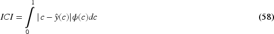
The empirical ICI is:

A metric related to ICI is the error percentile (EP) metric, also called EX (Hagopian et al., 2023). This is the
ICI, EP, and Emax have advantages over other ways of measuring calibration: they have a simple interpretation and assign a greater weight to dense data areas, which suppress poor estimates from sparse areas. The three metrics were compared by Austin and Steyerberg (2019) using simulated data with known ground truth while examining the performance of correctly and incorrectly specified models. ICI tends to demonstrate more consistent behavior in tests than EP or Emax.
5.9. Estimated Calibration Index
The estimated calibration index (ECI; Van Hoorde et al., 2015), also called the expected calibration index in Maier-Hein et al. (2024), is similar in concept to ICI. The definition is:

In equation (60), the calibration map
5.10. Fit on the Test
Kängsepp et al. (2025) define a general FOTT paradigm, where parameters of a calibration function from a family of functions are fit to the data by minimizing the ECE-FOTT loss in equation (22) through cross validation. Section 4.5 describes how bin-based schemes are a particular family of functions, leading to the tilted-roof reliability diagram. Curve-based function families have also been assessed using this paradigm, as described below.
The piecewise linear (PL) method for evaluating calibration fits a PL calibration map
The PL in logit-logit space (PL3) method fits a continuous PL function to logit functions
Other families tested under the FOTT paradigm include ECE-EM, Platt scaling, beta scaling, isotonic regression, spline fitting, and intraorder preserving functions (Kängsepp et al., 2025).
FOTT metrics have been assessed both with synthetic data, where the true calibration map is known, and with real data, where the true calibration map can be estimated accurately when there exist magnitudes more data than used in computing the calibration metric under test. The dataset CIFAR-5m contains 5 million synthetic images created so that models trained on the CIFAR-10 dataset have similar performance and vice versa. Metrics are assessed based on three objectives: (a) the quality of the reliability diagrams; (b) the quality of the calibration error estimates; and (c) Spearman's rank correlation between the metric ranks and the (approximately) true calibration error ranks, when assessing recalibration methods. For objective (a), PL is the best metric on average, followed by PL3 and beta scaling. However, the beta scaling rank gets worse as the number of datapoints increases due to the small number of parameters in the model. For objective (b), the 15-bin ECE-EM or beta metrics are the best, depending on the task. PL and PL3 also perform well. For objective (c), isotonic regression is best followed by 15-bin ECE-EM. PL is better than average and outperforms PL3 (Kängsepp et al., 2025).
The above assessment does not provide a clear ranking of calibration metrics as the ranking varies by objective. However, PL generally ranks well, and 15-bin ECE-EM also surprisingly ranks well, especially for the important task of ranking recalibration methods. Since ECE-EM is now considered a “classical” method and PL is relatively easy to compute, these should be considered for use generally. In passing, it is noted that the extensive experiments by Kängsepp et al. (2025) required over 10,000 hours of computer time to complete. Thus, it would be costly to recreate similar bespoke experiments for new projects.
5.11. Cox Intercept and Slope
The Cox intercept and slope (CIS) method measures calibration by performing a regression of the observed outcome against the log odds of the predicted confidence (Huang et al., 2020):

Perfect calibration has intercept
The CIS method has some similarities with the PL3 method, with the fitted function for CIS being equivalent to the fit for PL3 with a single segment. However, ECE-PL3 computes an ECE-style measure of the area between the fitted curve and the line of perfect calibration, whereas CIS analysis looks at the values of the intercept and slope to understand calibration. Although CIS provides more information than ECE-PL3, the need to analyze two variables makes CIS harder to use when assessing multiple recalibration algorithms automatically, like the above/below ABC metrics (Section 4.5).
5.12. Hypothesis-Test Kernel or Curve-Based Metrics
The statistical beta calibration test (SBCT) fits a beta calibration curve

The p-value is approximated by the quantile of A within the distribution
The parabolic Wald statistic (PWS) is defined by Galbraith and Van Norden (2011). A hypothesis test based on this statistic fits a parabola

The PWS metric takes on nonnegative numbers, is asymptotically distributed according to the chi-squared distribution, and standard significance tests can be constructed based on this. This statistic assumes the calibration curve may be well approximated by a parabola. This may be the case for some datasets but is not in general true if the calibration curve has a more complex character.
Gweon (2023) describes a Pearson chi-squared reliability statistic based on k-nearest-neighbors in the confidence prediction space and a Bayesian approach for estimating the expected power of the reliability test for different sample sizes. The use of nearest neighbors makes this metric reminiscent of kernel methods and ECE-KNN.
6. Cumulative Metrics
6.1. Empirical Cumulative Calibration Error
Reliability diagrams are usually based on binned estimates or sometimes kernel estimates, but the selection of width parameter for either type of representation can be arbitrary. Cumulative metrics sort datapoints by confidence and examine the difference between the cumulative accuracy and the perfect calibration line. The advantage of such metrics is that there is no need to set or estimate arbitrary parameters, such as bin width or curve parameters. Avoiding arbitrary choices helps when using metrics for regulatory compliance. The cumulative difference plot (CDP) is defined as

For a perfectly calibrated classifier, the CDP approximates a horizontal flat line at zero.
Two types of empirical cumulative calibration error (ECCE) are defined by Arrieta-Ibarra et al. (2022). The first is the maximum absolute deviation (MAD) of the CDP from zero. This is known as ECCE-MAD or the KS statistic.

The second error type is the range of the CDP. This is known as ECCE-R or the Kuiper statistic.

The variance of

The statistic
In Arrieta-Ibarra et al. (2022), the ECCE metrics are assessed and compared with standard ECE using synthetic data, where ground truth statistics can be computed. It is shown that the ECCE metrics can distinguish calibrated and miscalibrated classifiers as the number of samples grows large, but this is not the case for ECE. Analysis of classifiers applied to real datasets with many datapoints produces very low p-values for ECCE showing that such classifiers are statistically significantly miscalibrated. However, the effect size is small, as seen by the unnormalized ECCE statistics.
Gupta et al. (2021) define the KS calibration metric and describe it as a “binning-free calibration measure.” The final form of this metric is identical to ECCE-MAD, but it is derived in a slightly different way. A generalization of the metric also allows the assessment of whether the
The KS error is zero for perfect calibration and unity for completely uncalibrated systems. The metric can be construed as a percentage difference between two distributions, which aids interpretation of the metric. KS error can be shown to be a special case of kernel-based measures. The relationship between KS error and the cumulative distribution function (CDF) is the same as the relationship between MCE and the binned probability density function—they are both based on the maximum difference (Roelofs et al., 2022).
KS error is compared to RBS, ECE, and CWCE by Gruber and Buettner (2022). Only KS and RBS are consistent in value with respect to data size. KS error is used, along with ECE, KDE-ECE, MCE, and BS by Gupta et al. (2021) to assess various recalibration methods on an ImageNet recognition challenge. All metrics give similar rankings for the best recalibration methods. However, since the ground truth for this challenge is not known, it is not possible to determine which metric is best.
6.2. Cumulative Multi-Calibration Metric
Guy et al. (2025) discuss the concept of multi-calibration, which is to make sure that all specified subpopulations of the full dataset are calibrated. The Q, possibly overlapping, subpopulations could be bins based on confidence, groups of datapoints that have similar feature values (if it is desired that all parts of the feature space are calibrated), or a combination of both. The authors propose a metric to measure the multi-calibration error, which is computed as follows. Let

Equation (68) is a weighted version of equation (64), but only for a single subpopulation. A Kuiper statistic for the subpopulation is then computed as:

The multi-calibration metric (MCM) is defined as the worst-case Kuiper statistic weighted by its signal-to-noise ratio under the hypothesis of perfect calibration, assessed over all specified subpopulations:

The general MCM metric can be used with any specification of subpopulation. One specific use case could be to analyze the treatment of people according to protected characteristics to ensure that any automated decision systems are well calibrated for all such characteristics. However, Guy et al. (2025) describe an optional automated method for generating subpopulations based on using a binary tree to partition the data using feature values. The method retains all internal nodes of the tree, resulting in overlapping subpopulations.
The range of MCM is
6.3. Brownian Bridge Test
Sadatsafavi and Petkau (2024) specify a hypothesis test that makes use of the equivalence of CDPs with BM. The test is generally more powerful than that based on ECCE-MAD. The test is based on a Brownian bridge, as follows. Let


The maximum absolute value of the bridged random walk is:

The Brownian bridge test (BBT) p-value is then:

In equation (74)
BBT was compared to the p-value produced by the ECCE-MAD hypothesis test of Arrieta-Ibarra et al. (2022), which is referred to as the BM test in Sadatsafavi and Petkau (2024). In small test datasets with an effective sample size of less than 30, the p-values of both methods are slightly biased upwards, so the tests are conservative (i.e., reject fewer tests than expected). BBT was more powerful than BM in all cases other than with pure mean shifts in calibration, and in those cases the power was only slightly lower (Sadatsafavi & Petkau, 2024). Based on these results, BBT should be preferred to BM.
7. Conclusion
7.1. Summary
This article analyzes the wide range of metrics used to assess the calibration of probabilities produced by ML models and organizes these metrics according to families: point, bin, kernel, curve, or cumulative metrics. For each family, Table 1 shows the number of metrics identified, how many have different nominal ranges of value, how many are proper, how many have a built-in associated hypothesis test, and the number that distinguish underconfidence from overconfidence. A list of general pros and cons for each family is shown in Table 2.
Summary of Calibration Metric Families.

General Pros and Cons for Each Calibration Metric Family.

ECE = expected calibration error.
Table 4 in Appendix D summarizes all the individual metrics discussed in this article. For each metric, the table lists: alternative names; family; value range; whether the metric is proper; whether a hypothesis test is available; whether they distinguish underconfidence from overconfidence; and pros and cons.
7.2. Analysis and Recommendations
With so many metrics to choose from, it is necessary to recognize good metric properties to aid their selection. Hagopian et al. (2023) define various characteristics that good calibration metrics should have, including reproducibility, representativeness, interpretability, parsimony, and computational efficiency. Three further potentially useful properties are cataloged in Table 4. Being proper or having a hypothesis test are advantages of a metric but are not necessary for its use. The third property of being able to distinguish under from overconfidence is a major advantage, but lack of this characteristic does not exclude the metric, depending on the use case. Further properties only applicable to certain metrics appear in the pros and cons columns of Table 4.
No single metric is better than all others, as each one has advantages under certain conditions. Summaries of various numerical comparisons are included in the individual metric descriptions above. However, each comparison only covers a small subset of all metrics described so it can be difficult to assess the complete portfolio of possible metrics. Nevertheless, recommendations can be made for a series of use cases.
The first use case is to have a metric that is generally applicable for classifier probability calibration and is used to assess the class-wise calibration performance of models or calibration improvement of recalibration algorithms. To avoid conflating the assessment of accuracy and calibration a pure calibration metric should be selected. Such a metric should at least have Hagopian's properties. One candidate is the standard equal-width
Binned metrics can be “gamed” by models that set all confidence values to a single value or vector equal to the class proportions, producing good outputs according to the metric but not necessarily useful. Several authors, for example, Chidambaram and Ge (2025) and Silva Filho et al. (2023), therefore recommend that a proper score should be reported alongside any binned metric. The top two choices would be the BS or NLL due to their widespread use and understood properties. As discussed in Section 3.4, log metrics are highly sensitive to the presence of confidence values near zero, violating the representativeness criterion. Therefore, we recommend that the BS should be reported along with DRMSCE-BCS.
The second use case is full multiclass calibration. DRMSCE-BCS cannot be used for this purpose—no bin-based metrics have a reasonable extension to full multiclass calibration with
The third use case is determining whether miscalibrated classifiers are under or overconfident. Several metrics meet this high-level requirement. Of the point-based metrics, EO is the only one not to have sensitivity to specific confidence values like ECD, NSES, or the Spiegelhalter z statistic. However, as a global metric EO lacks refinement. From the bin-based metrics, ESCE is preferred as it has a simple definition and there is no clear benefit to the more complex DICI and WSMCS. The variant of ESCE by Verhaeghe et al. (2023) that averages over different bin widths should be used to reduce bias. Consideration should be given to an EM extension to further reduce bias. If it is required to determine under and overconfidence separately, then the bin-based ABC should be used. The kernel-based SCE has a slightly complex definition and thus lacks interpretability. The curve-based CIS has a simple definition, but requires the analysis of two parameters, which complicates analysis. Based on the above analysis, we recommend ESCE as a single metric to measure under and overconfidence.
The fourth uses case is to measure the stronger notion of local calibration, where feature values are used in the assessment. Several metrics meet this high-level requirement: the bin-based PIECE, PCE, multi-view calibration error (MVCE), FECE, and VECE; the kernel-based KLCE and ECMMD; and the cumulative MCM. The metrics ECMMD and MVCE contain a random sampling element, harming their reproducibility. FECE and VECE use only one confidence bin, resulting in a global confidence metric for each feature-partition of the data, and an ensuing lack of refinement in confidence analysis. KLCE is the only metric that allows assessment of full multiclass calibration, and it has a defined hypothesis test based on boot strapping. KLCE is unbiased and is smoother than the remaining bin metrics of PIECE and PCE. The major disadvantage of KLCE is its sensitivity to the choice of kernel and how its hyperparameters are optimized. PIECE bins data in feature space by density. While this allows miscalibration detection in the presence of cancelation between different parts of the feature space, the location of miscalibrated areas cannot easily be identified. Based on the analysis above, we recommend a specialization of the general PCE metric that uses
The fifth and final use case is for developers and researchers to perform deeper analysis beyond the use of a single numerical metric for automated comparison and assurance. Models may be under or overconfident at different confidence levels. These variations in calibration can cancel each other out to different extents depending on the metric, resulting in ostensibly good metric values that mask a more subtle issue (Van Calster et al., 2024). Therefore, for refined analyses it is recommended that calibration curves with associated confidence intervals should be plotted on the reliability plot, like in Figure 3, and examined.
7.3. Further Work
This article has outlined the definition and properties of many metrics. Existing comparisons between metrics typically only assess a small number of metrics at a time, and these comparisons are often carried out by metric designers who perform analysis from an angle that may be beneficial to their metric. A large-scale independent study should compare the more promising metrics in this survey using data and models of known levels of miscalibration.
Certain specific lines of research would be useful. DRMSCE-BCS is a recommended metric for top-label and class-wise calibration but is not applicable to full multiclass calibration. A debiasing term and automated binning strategy should be developed for the multiclass setting, including an analysis of scalability as the number of classes grows. Sun et al. (2024) show that the distribution of
This survey focuses on the probability calibration of classifiers that produce confidence scores for a fixed set of unordered classes. Similar surveys should be carried out to catalog probability calibration metrics for other problems, including object detection, conformal classification with variable numbers of output classes, ordinal classification for ranked classes, and regression.
Finally, several open problems in probability calibration assessment are discussed in Silva Filho et al. (2023). These include characterising the epistemic uncertainty in models and assessing out-of-distribution inputs. These topics should be investigated further from a calibration point of view.
Footnotes
Acknowledgments
The author thanks Emma Tattershall, Sarah Pengelly, and William Wood for productive discussions about probability calibration issues and for reviews of early versions of this survey.
Ethical Considerations
Not applicable.
Consent to Participate
Not applicable.
Consent for Publication
Not applicable.
Funding
The authors disclosed receipt of the following financial support for the research, authorship, and/or publication of this article: Funding for initial literature survey and write-up activities was provided by the Defence Science Technology Laboratory (DSTL) under Task 267 in the Analysis for Science and Technology Research in Defence contract DSTL/AGR/01142/01. Subsequent survey activities and the production of this article were funded by the QinetiQ Fellow scheme.
Declaration of Conflicting Interests
The author declared no potential conflicts of interest with respect to the research, authorship, and/or publication of this article.
Data Availability
Since this article is a review article, no datasets are analyzed or generated other than for illustrative purposes.