Sage Journals: Discover world-class research

Abstract

Recently, the European Union adopted a Nature restoration law that aims to stop the ongoing decline of biodiversity and even bring back nature to cities. This is challenging as urbanization is an ongoing process that thrives for more land and densification. In this paper we describe a new Open-Source GIS-tool that automates habitat network analyses and simultaneously generates several maps that can be used for assessments, targeting species survival in urban environments. One result of particular interest is the habitat functionality map that combines values of habitat quality and connectivity. We tested the tool’s ability to predict habitat functionality using amphibian occurrence data observed from the city of Gothenburg in Sweden. Our evaluation shows that habitat functionality was generally a good predictor of amphibian distribution. However, the predictability was sensitive to the cartographic representativity of the input biotope map used. Also, predictions of habitat functionality improved when estimating dispersal probabilities using the Cost-distance algorithm, compared to when using Euclidean distance from reproductive habitats. This finding supports the need to use connectivity models that are responsive to variation and changes in roads, traffic volumes and buildings when performing effect analyses on biodiversity in cities. Finally, we demonstrate how the tool can be used to easily identify areas where restoration measures can effectively increase habitat functionality for target species. This can help planners to find efficient solutions for increasing biodiversity within urban areas.

Keywords

Habitat connectivity restoration habitat quality animal dispersal road barrier green infrastructure GIS cost-distance Amphibia place syntax tool

Introduction

We urgently need to improve the way that cities are planned to minimize losses of biodiversity and improve the quality and functionality of habitats within urban areas (Balfors et al., 2016). Recently, the EU adopted the Nature Restoration Law, which aims to increase biodiversity and secure the prerequisites for all valuable ecosystem services within at least 20% of the land and sea areas by 2030, and ultimately for all ecosystems in need of restoration by 2050. In urban areas, the goal is to have “no net loss of green urban space by 2030, and an increase in the total area covered by green urban space by 2040 and 2050” (https://environment.ec.europa.eu/topics/nature-and-biodiversity/nature-restoration-law_en). This is especially challenging as urbanization and densification of urban areas are expected to continue. Hence, we need to find effective ways to improve the ecological functionality of the green and blue infrastructure within cities consisting of all natural and semi-natural biotopes on land (green areas) and aquatic environments (blue areas). This calls for practical, effective and reliable tools that can be used by planners to estimate habitat functionality and connectivity for many types of organisms at the same time.

When analysing the effects of urbanization on the functionality and connectivity of habitats, the models used must be responsive to the planned environmental changes. This includes transformations in transport infrastructure, built-up areas and the biotope composition of green and blue areas. It is also beneficial if the modelling framework used can be generally applicable to all existing species groups independent of the spatial scale of the planning project. Many of the established methods for ecological modelling, such as metapopulation models and other spatially structured population models, do not really fulfil these prerequisites. These types of models can respond to habitat loss or habitat quality changes (Akҫakaya et al., 2004; Hanski and Gilpin, 1997), which make them very useful for large scale risk assessments and species conservation plans (Burgman et al., 1993). However, almost without exceptions (e.g., Kindvall, 2000), metapopulation models handle movements of individuals as a negative exponential function of Euclidean interpatch distances (Akҫakaya et al., 2004; Hanski, 1999). This makes these models insensitive to barrier effects that may arise when changing the interpatch environment by building more houses or by adding new transport infrastructure (Vergnes et al., 2014). Habitat suitability models, which are also commonly used when modelling species habitats (Hirzel et al., 2006), also lack the responsiveness to barriers as these models measure habitat quality without any consideration of connectivity.

Metapopulation models have been criticized for being applicable only at spatial and temporal scales that are appropriate for the focal species in mind (Thomas and Kunin, 1999). Furthermore, metapopulation models and many traditional habitat network models, where the landscape is simplified into habitat patches and dispersal links, require that habitat patches can be clearly distinguished from a surrounding non-habitat matrix. Thomas and Kunin (1999) concluded that most species do not fit into this simplification of the landscape. Hence, patch-based models are not generally applicable at all scales.

In accordance with Thomas and Kunin (1999), we conclude that a solution to the identified shortcomings of many of the patch-based models is to adopt a grid-based approach that can handle the continuous variation in habitat quality and connectivity at every point in the studied landscape. Raster-based habitat network models can handle barrier effects caused by transport infrastructure changes or other transformations in the urban landscape. This is done either by implementing the Cost-distance algorithm (Karlson and Mörtberg, 2015; Sahraoui, 2021) or electrical circuit theory (McRae et al., 2008). Although none of these approaches fully captures the mechanisms of animal and plant redistribution processes in relation to variation in landscape composition, they often produce predictions that fit observed patterns (McRae and Beier, 2007; Wang, 2021).

In most published habitat network models, the results from the raster-based modelling are summarized into a vector-based network consisting of different sized habitat patches connected by links describing the most cost efficient or averaged movement path (Heliodora, 2023; Sahraoui, 2021; Zetterberg et al., 2010). This approach makes it possible to apply several types of connectivity indexes, which are definitively useful when trying to evaluate which patches are the most important to preserve (Dallas et al., 2020; Keeley et al., 2021). However, here we will focus on an alternative type of habitat network analysis, i.e., raster maps showing estimates of habitat functionality that have only quite recently been described and tested (Van Moorter et al., 2023; Von Hirschheydt et al., 2020). This new raster-based approach handles spatial variation in habitat quality without the need to delimit habitat patches that are clearly separated from non-habitats. Habitat functionality is a measure that combines the estimated quality at every point in the landscape with its connectivity to neighbouring habitats in a way that is clearly in line with the solution suggested by Thomas and Kunin (1999).

In this paper, we describe a new GIS-based tool that can perform habitat network analyses automatically for a whole range of species or functional groups of organisms at the same time. We use observation data on amphibians to test the model’s ability to predict habitat functionality and dispersal probability. We specifically explore the sensitivity to the quality of the environmental input data. We also compare the predictability of the tool using two alternative sets of model parameters: one that makes the model responsive to biotope specific barrier effects using the Cost-distance algorithm and one that assumes dispersal being just a function of Euclidean distances. Finally, we demonstrate how the tool can be used when planning restorations aimed at improving the ecological functionality of green and blue areas in a city.

Methodology

Study area and organisms

We selected Gothenburg and its surroundings as a study area where the habitat network function could be tested. In this area several species groups are well represented among publicly available species observation data. We selected amphibians because they are a well-known group that uses both terrestrial and wet habitats, which makes them representative of the biodiversity living in both green and blue areas within cities.

We downloaded all observations of amphibian species from the Swedish Species Information Centre on 9 June 2024 (https://fynddata.artdatabanken.se). These data were collected mainly by volunteers but also by professionals doing specific surveys. Nevertheless, as these data are not collected in a standardized way (Leidenberger et al., 2016), they can at best be used to indicate where the species has been present at least once. In the absence of more robust data, here we use the public data to make a rough evaluation of the model predictions. Using t-test, we tested the accuracy of alternative model predictions by comparing mean habitat functionality estimated at places where amphibians have been observed in places without any known observations (see Supplemental Material).

Altogether, 911 observations, dated between 2000 and 2024, were included in the amphibian data set after selecting only records with at least 100 m accuracy. Half of the observations (46%) was made in small waters where amphibians can reproduce, while all other observations were made in different terrestrial biotopes. The data included three species of frogs (Pelophylax esculentus, Rana arvalis, Rana temporaria), one toad species (Bufo bufo) and two newts (Lissotriton vulgaris, Triturus cristatus). This is nearly half of all amphibian species occurring in Sweden, and only two more species exist in the vicinity of Gothenburg. To enhance visual comparisons between observations and model predictions, the observations were generalized into polygons representing areas where amphibians exist. This was made by buffering all observation points by 100 m. Here the observation data were used only for evaluation of the model predictions. The model parameters were set as described by Sahraoui (2021) based on expert opinions published on the SLU Swedish Species Information Centre’s home page (https://artfakta.se).

Software description

The software we test in this study is an original tool named the Habitat Network Analysis Tool (HNAT), a plugin for the open-source Geographic Information System QGIS (https://qgis.org/en/site/). The plugin is written in Python and is accessible via Github (https://github.com/SMoG-Chalmers/habitat-connectivity-tool). The plugin uses QGIS GDAL (Geospatial Data Abstraction Library) and GRASS (Geographic Resources Analysis Support System) via the QGIS processing framework for some of its calculations. The plugin adds a processing algorithm to the QGIS Processing Toolbox, which means that it can be used either directly from the QGIS Processing Toolbox or in QGIS Modeler.

HNAT supports analyses of species raster-based habitat networks including a multi-species approach, which is of special benefit when trying to develop plans that do not harm biodiversity (Sahraoui et al., 2021). It has been developed within the ongoing project ‘Development of a digital tool for integrated impact assessment of social, economic, ecological and cultural-historical values in transport infrastructure planning in urban environments’, financed by the Swedish government research funding agency FORMAS, which aims to create a practical software where socio-economic, ecological and cultural historical analyses can be integrated when exploring the effects of urban transformations, with a specific focus on different types of alterations in the transport infrastructure (Berghauser Pont et al., 2022).

Using just a biotope raster file and an Excel file with all model parameters, HNAT generates a whole set of useful output maps, which describes the spatial structure of the modelled habitat from the analysed organisms’ point of view (Figure 1). Furthermore, the set of output maps are automatically generated for each species or organism group specified in the parameter file.

Figure 1.

The habitat network analysis tool automatically generates a series of different maps (e.g., the friction map, the habitat quality map, the dispersal probability map, the habitat functionality map and polygon layers representing delimited source habitat patches and habitat network areas) based on an input biotope map and an Excel file including all organism and biotope specific model parameters. Blue arrows indicate the sequential process of how the maps are generated.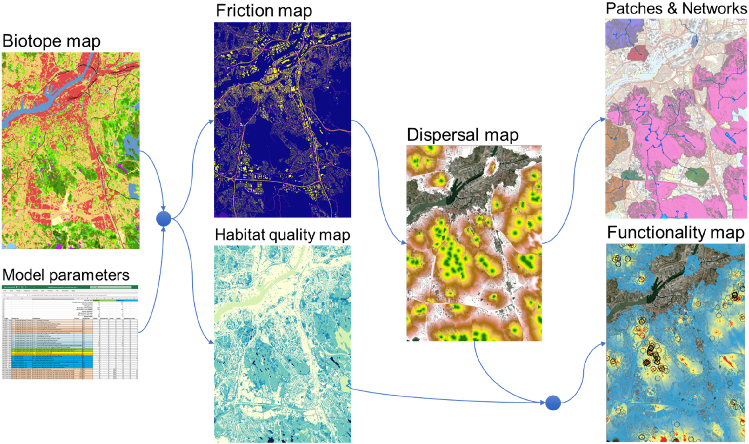

Preparation of input biotope map

HNAT requires a raster file (GeoTiff-format) as input, where pixel values correspond to specific biotopes or environmental elements. Any kind of land cover map, which describes the biotope composition of the study area, could be used as an input map. However, in many cases, model predictions are expected to become more realistic if the basic land cover map is complemented with other sources of environmental information that are relevant for the selected focal organism. Examples of such information include soil or bedrock maps, soil moisture, altitude, slope directions, etc.

In this case, the Swedish land cover map (https://geodata.naturvardsverket.se/nedladdning/marktacke/NMD2018/NMD2018_basskikt_ogeneraliserad_Sverige_v1_1.zip) was modified to achieve a greater cartographic representation of both buildings and transport infrastructure as these environmental elements can generate different levels of mortality and barrier effects on the modelled organisms depending on building height or traffic volumes.

In total, 20 new biotope classes representing buildings of different height ranging from less than 5 m up to 100 m, were added to the basic land cover map. The heights were obtained by analysing the LiDAR data provided by the Swedish Land Survey; for details, see Berghauser Pont et al. (2019). The data were rasterized and added on top of existing pixels representing buildings in the Swedish land cover map.

Roads were separated into 101 new biotope classes with different expected numbers of vehicles per day. Instead of using statistics from the Swedish Transport Administration on the observed number of vehicles per day, we used angular betweenness centrality values calculated from the road network using PST (Place Syntax Tool, Stavroulaki et al., 2023). PST is an open-source plugin for QGIS (https://smog.chalmers.se/projects/pst-plugin-for-qgis). As the traffic volumes are expected to be correlated with the centrality values (Serra and Hillier, 2019) it is often a better option to use these, as values can then be obtained for all roads and not only the ones that have been surveyed. This is especially valuable when modelling future scenarios where only predicted traffic volumes are available for use. Angular betweenness centrality is a measurement of centrality that is based on the angular structure of paths in a network instead of its metric properties (Omer et al., 2017).

The vector layer with the centrality values was buffered by 15 m prior to rasterization. The new pixel values were then added to the basic land cover raster in sequence, following the order of the centrality values. This was done to avoid road pixels representing relatively high centralities to be overwritten by lower road classes. If this procedure is not applied, there will be an obvious risk of underestimating barrier effects by the habitat network model at places where roads are located along side each other, or where they cross.

In addition to information on specific barriers, we also added information on small streams with a maximum width of 6 m. Such small streams are not represented in the Swedish land cover map as the pixel resolution is 10 × 10 m. Adding streams to the biotope map is expected to increase predictability of the habitat network model for amphibians as these are known to disperse through the landscape along the streams. Three classes of smaller streams were obtained directly from a vector layer of Swedish streams (https://www.lantmateriet.se/en/geodata/geodata-products/product-list/topography-50-download-vector/). These lines where rasterized and added to the land cover raster by replacing the original pixel values with new values representing each type of stream.

Finally, we added the possibility to discriminate between smaller pondlike waterbodies and bigger lakes and broad streams. This was done in two ways: 1) by manually reclassifying the existing pixel values of the biotope class named “Inland water surfaces”, which originally includes only waters above 100 m²; 2) by adding small waters from OpenStreetMap (n = 63 additional ponds).

Setting organism specific model parameters

In the HNAT input file, three species specific parameters must be specified separately for each biotope class existing in the biotope map. These parameters are Quality, Reproduction and Friction.

Quality (Q) is an integer value ranging from zero to infinity which should correspond to the relative habitat quality of each listed biotope. Biotopes that do not have any resources that can be used by the target species should have the Quality set to 0 while the biotope used for foraging, reproduction or hibernation should be set a positive number reflecting its relative importance or temporal availability. A lower value could be set on a feeding biotope if food items only occur there during a shorter period compared to a biotope that can be used for feeding all through the season. The habitat network method will generate a Habitat quality map (Figure 1) by replacing the biotope class values with the specified biotope specific quality values.

Reproduction is a parameter that can be set to either 1 or 0 depending on whether the biotope is used for reproduction or not. As biotopes used for reproduction will be the origin for dispersal of all juveniles, we define these parts of a specie’s habitat as the source habitat. In the modelling process, dispersal will originate from the identified source habitats from which all individuals of the target species are expected to emerge, and to which adults return every breeding season to reproduce. HNAT automatically generates a layer that delimits all source habitat patches based on the pixels representing biotopes where reproduction is set to 1.

Friction is an integer value ranging from 1 to infinity which should correspond to the relative barrier effect (θ) that each biotope imposes on the modelled dispersal. All biotopes where the target species can move freely should have the value set to 1. When moving through a biotope where the friction (θ) is greater than 1, the total distance reached will be equal to 1/θ times the distance reached moving within the biotopes where dispersal is not restricted. The habitat network method will generate a Friction map (Figure 1) by replacing the biotope class vales found in the Biotope map with the specified biotope specific friction values (θ).

The general parameters that must be specified for each modelled species regulate the capacity of dispersal from source habitats. The Average dispersal distance (D) will determine how fast the dispersal probability will decline with distance from the source habitat pixels. The Network threshold is specified as the minimum interpatch dispersal probability (P_n) that is required within a network to make separate source habitat patches functionally connected demographically or genetically. If the dispersal probability between two source habitat patches falls under this threshold, then the source habitat patches will belong to separate habitat networks. Setting this parameter to very low values can be useful when trying to identify separate metapopulations (Hanski, 1994), while higher values may give ideas on how populations are structured into local populations of different sizes (Hanski and Gilpin, 1997).

Estimating road barrier effects based on predicted traffic volumes

In the habitat network model tested here, barrier effects are specified by setting biotope specific friction parameters that are used when calculating pixel specific Cost-distances from source habitats. The higher the friction, the greater the barrier it will be for the modelled organism to cross over while dispersing through the landscape.

Roads can have negative effects on populations by acting as barriers for dispersal but will often also impose a severe risk of mortality. Both these effects will lead to increased isolation between different parts of a specie’s habitat (Ceia-Hasse et al., 2018). It is expected that this risk will increase with traffic volumes. As traffic volumes can be predicted by centrality values of road networks (C), we used the Angular betweenness centrality measure, which can be calculated using PST, when estimating friction values (θ) for roads. To do this we applied equation (1) as follows:

θ = R o u n d [θ_{\min} + (θ_{\max} - {B θ}_{\min}) \times {(\frac{C}{C_{\max}})}^{μ}]

(1)where C_max is the maximum centrality value generated within the study area, and θ_min and θ_max denote the minimum and maximum expected friction values, respectively.

The parameter µ is an exponent that will affect the shape of the relationship between friction and expected traffic intensity. If set to values greater than 1, the friction will initially increase slowly with centrality, but eventually become very high rapidly when centrality increases. If set to less than 1, friction will increase rapidly at low traffic volumes and then level off. If µ is set to 1, the barrier effect will increase linearly with the increasing centrality. For the amphibian species analysed, we set μ = 0.6 and θ_min and θ_max to 2 and 100, respectively.

Estimating barrier effects from buildings based on heights

Buildings can potentially be great barriers for dispersal, but the effect may be very different depending on the type of organism. Flying insects may experience an increased barrier effect related to building height (Mayrand and Clergeau, 2018), while amphibians will experience the same barrier effect independent of height. Potentially, equation (1) can be used also for calculations of friction values from building heights (H). To do this, one can replace C with H.

Ground dwelling species, like amphibians, must walk around the buildings no matter the actual height to reach the other side. For this kind of organisms, friction should be set to a relatively high value. In this study we set the friction (θ) of all buildings to 1000.

Calculating dispersal probabilities

HNAT models dispersal from all identified habitat patches in three steps. First a Friction map (Figure 1) is generated by simply replacing the pixel values of the input Biotope raster with the biotope specific friction parameter values (θ) specified in the input file for the modelled species. Using the Friction map as the input raster to the GRASS function r.cost, a new raster is generated where each pixel value represents the cost weighted distance from the nearest source habitat pixel. This map is called the Cost Distance map. Finally, the Dispersal probability map is generated using equation (2), which represents the negative exponential dispersal function in most spatially structured population models that have been used by ecologists (e.g., Hanski, 1994):

P_{d} = e^{- \frac{D_{c}}{D}}

(2)where the dispersal probability (P_d) is here calculated directly from the pixel values (D_c) in the Cost Distance map and the species-specific parameter D, which denotes the average dispersal distance normally performed by the focal species.

Calculating habitat functionality

The ecological functionality at a certain place is not just a function of how useful the biotope or the existing resources are for the organisms potentially using it. The resources must also be reachable from other places that organisms need to visit every now and then. For example, an area with plenty of food items is not functional if it is situated too far away from the nearest source habitat where the organism can reproduce. Thus, functionality is dependent both on the quality of the habitat and how connected it is with other essential landscape features. In the current habitat network model, the pixel values of the Functionality map (F) are calculated by simply multiplying each pixel value (Q) in the Habitat quality map with the corresponding pixel value in the Dispersal probability map (P_d):

F = Q \times P_{d}

(3)

Results

Validation of model predictions

Initially, three versions of the model predictions were generated for the whole study area including Gothenburg city and its surroundings. These versions differed in the amount of input information added to the Swedish land cover map regarding different types of freshwater biotopes. Most of the amphibian observations were seemingly well associated with areas where the investigated habitat network models predicted relatively high dispersal probabilities (Figure 2) and habitat functionality (Figure 3), using the model where dispersal is affected by biotope specific friction values. The mean habitat functionality differed significantly between locations where amphibians have been observed and positions without any known observations according to t-test using all three biotope maps (Table S1). However, predictability was clearly sensitive to the selection of the input biotope data.

Figure 2.

Amphibian observations plotted on three alternative maps with predicted dispersal probabilities. The maps have been generated based on different input biotope maps: (a) Only the original land cover freshwater biotope class; (b) Manual categorization of freshwater classes into ponds and others; (c) Land cover map complemented with ponds from OpenStreetMap.

Figure 3.

Amphibian observations plotted on three alternative habitat functionality maps in Gothenburg. The maps have been generated based on different input biotope maps: (a) Only the original land cover freshwater biotope class; (b) Manual categorization of freshwater classes into ponds and others; (c) Land cover map complemented with ponds also from OpenStreetMap. Habitat functionality is calculated by multiplying the biotope quality with the dispersal probability (equation (3)).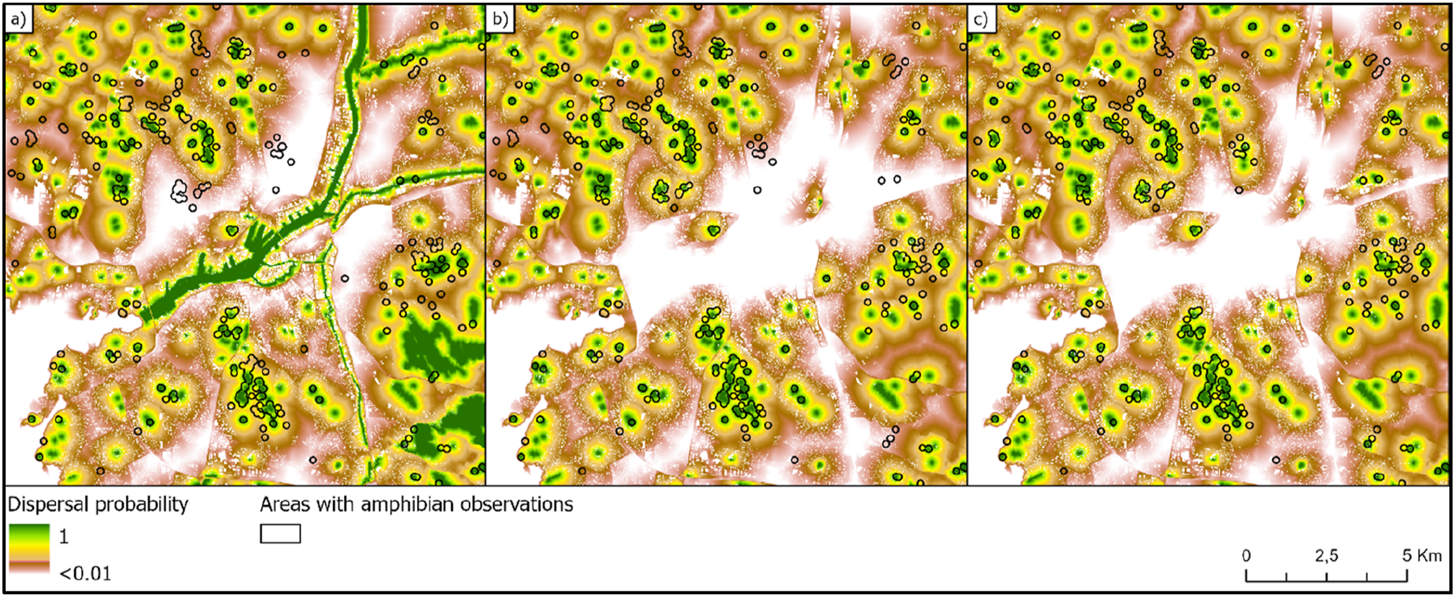

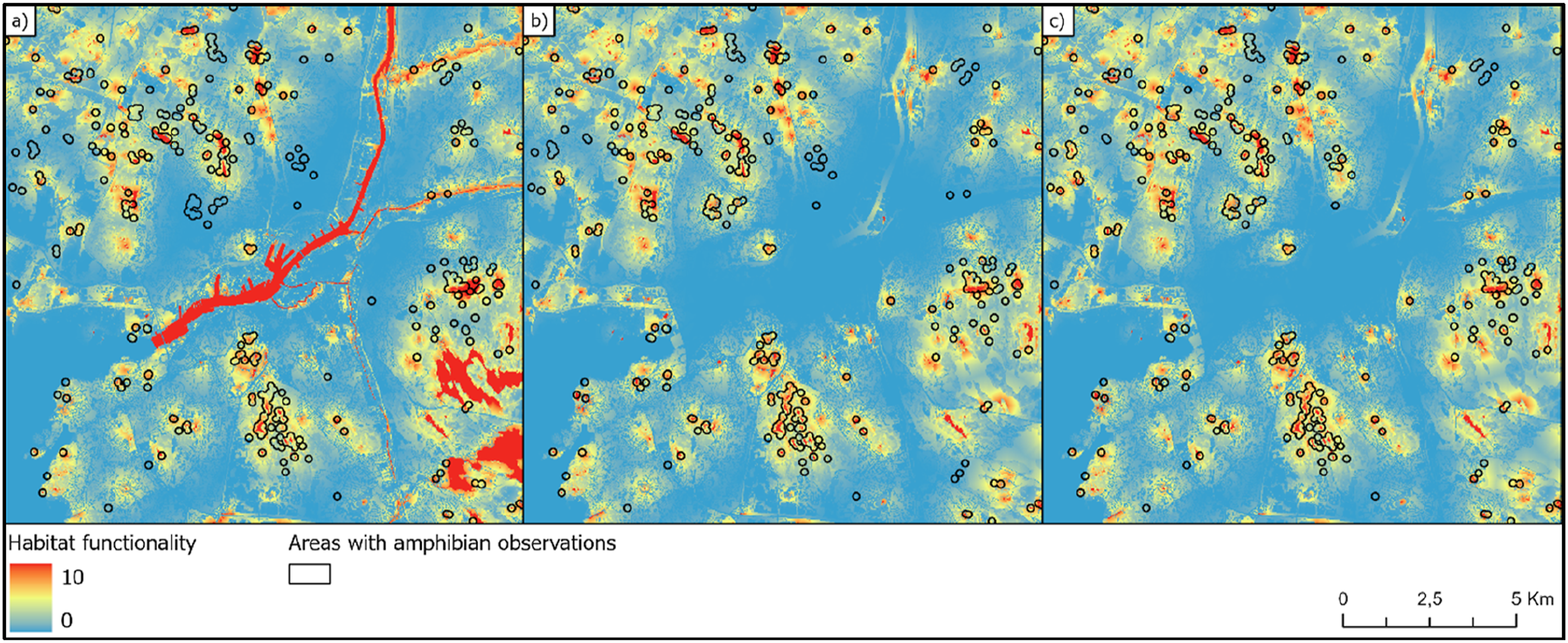
When using only water information from the original version of the Swedish landcover map, several examples of apparent mismatches were found when comparing areas with amphibian observations with predicted dispersal probability (Figure 2(a)) and habitat functionality (Figure 3(a)). Several of these mismatches disappeared when the predictions were based on biotope maps where small water bodies were separated from bigger streams and lakes (Figures 2(b), (c), 3(b) and (c)). Comparing the t-statistics from the t-tests on habitat functionality, model precision became twice as good when extra ponds were added based on data from OpenStreetMap compared to when using the unmodified landcover map as input (Table S1). Adding the extra ponds from OpenStreetMap made the model prediction almost 10% better than when only separating waters by size in the original landcover map (Table S1).

To investigate the importance of using Cost-distance when performing habitat network analyses, the amphibian model was altered by setting all friction parameters to 1 for all biotopes. This change generates Euclidian distances for the dispersal calculations instead of Cost-weighted distances. This results in a less restrictive dispersal pattern within the study area (Figure 4(a)). According to the t-tests on mean habitat functionality, both alternative dispersal models generated predictions of habitat functionality that significantly discriminate areas where amphibians have been observed from areas without known observations (Table S2). Both models proved to be at least 87% better at predicting amphibian occurrences than a model that only considers the habitat quality, completely ignoring connectivity among pixels (Table S2). The model based on Cost-distances was only 2% better than the model that was based on Euclidian distances according to the t-statistics on mean habitat functionality (Table S2). However, the total area of habitat with functionality values above 3.0 was 20% (839 ha) larger when using Euclidean distances (Figure 4(b)) instead of Cost-weighted distances (Figure 3(c)). Despite this, only 0.7% more observations were reported from the additional areas predicted by the more inclusive model. It is also striking that no observations occur in areas where functionality increases when using Euclidean distances instead of Cost-weighted distances (Figure 4(c)).

Figure 4.

Predictions of dispersal probability (a) and habitat functionality (b) assuming dispersal probabilities being only a function of the Euclidian distance from the source habitats. As the maps were generated based on the biotope map with extra ponds from OpenStreetMap, a) and b) can be compared with Figures 2(c) and 3(c), respectively. Areas with observations do not overlap with areas where habitat functionality increases when biotope specific friction is ignored (c).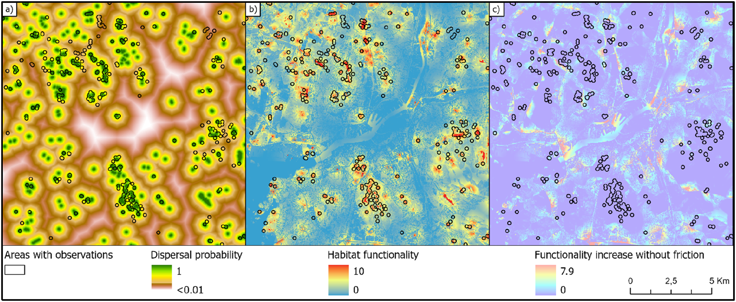

Identifying restoration areas

To demonstrate how the current habitat network model can be used when planning restoration actions, we used the results from the model that had the best fit to observed data. By simply subtracting the pixel vales in the Habitat functionality map (Figure 3(c)) with the values of the corresponding pixel in the Habitat Quality map (Figure 5(a)), we obtained a Difference raster where high pixel values indicate areas where habitats with high quality are not functional due to the lack of connectivity in relation to nearest source habitats where amphibians can reproduce (Figure 5(b)). By selecting all pixels in the Difference map exceeding 6.5 within continuous areas greater than one ha, we generated a polygon layer delimiting areas with the greatest potential for restoration measures (Figure 5(c)).

Figure 5.

The difference between the habitat functionality map (Figure 3(c)) and the corresponding Habitat quality map (c) generates the highest values where quality is high but where dispersal is limited (Figure 2(c)). Based on the calculated differences (b), areas potentially suitable for habitat restoration were selected (c).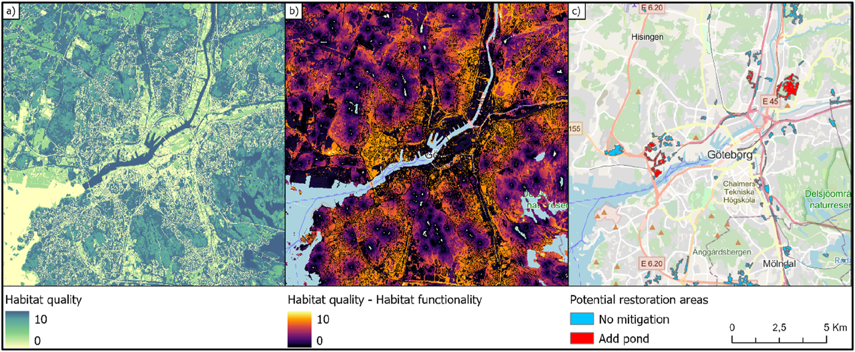

Effects of proposed restoration actions

We performed a scenario analysis where a proposed restoration solution (Figure 6(a)) could be evaluated in relation to the current situation. We identified areas that have great potential for improvements in Habitat functionality. From these areas we selected the eight largest for testing the effect of constructing new ponds suitable for amphibians to reproduce. One pond per selected area was implemented as a restoration action in the future scenario (Figure 6(a)).

Figure 6.

Results from scenario analyses where the effect of creating new ponds for amphibians can be evaluated in terms of increased habitat functionality. The increases from current (b) to the future situation (c) occurred also far from the selected restoration areas (a) where the creation of new ponds was proposed.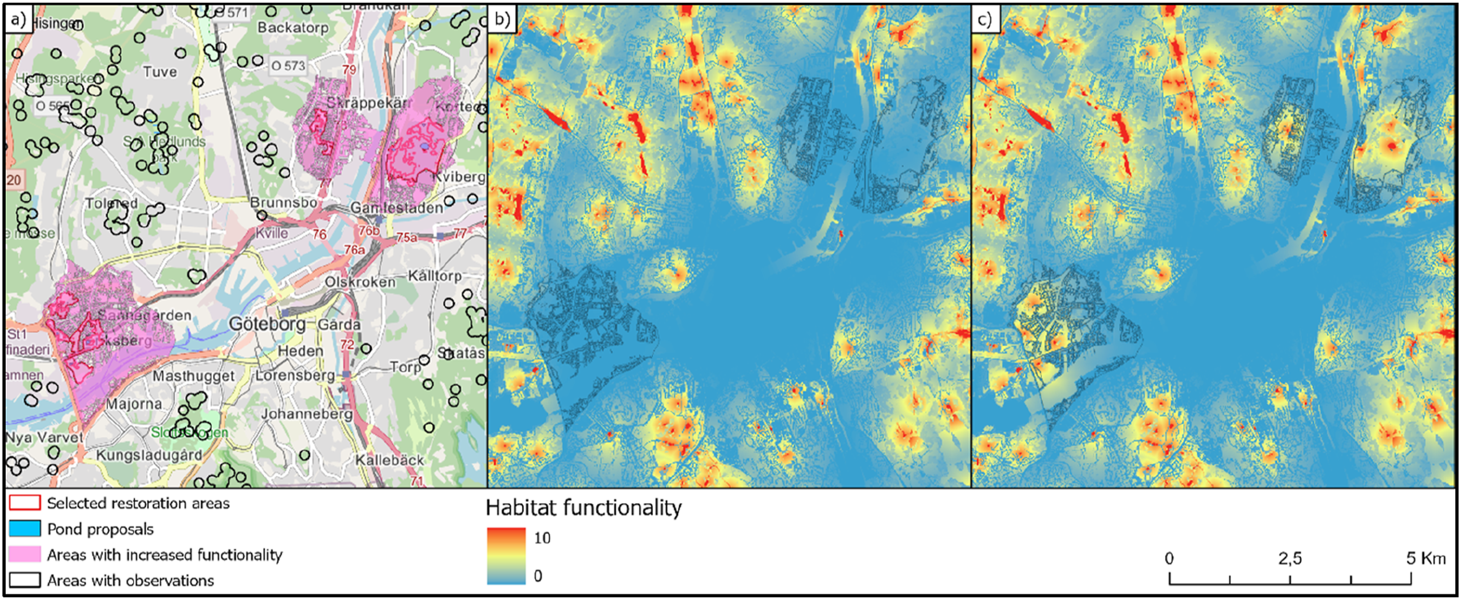

The Functionality map representing the current situation (Figure 6(b)) can be compared with the corresponding Functionality map that represents a future scenario when the restoration plans have been implemented (Figure 6(c)). Subtracting the pixel values in the Functionality maps from the two scenarios gives a measure of the expected effect that the planned restorations can have on amphibians within the city of Gothenburg. In this case, the total functionality increased more than seven times within the areas affected by the restoration. The areas where Habitat functionality was affected according to the scenario comparison are apparently bigger than the selected restoration areas where ponds were created (Figure 6(a)). Note also that there is no overlap between areas where amphibians are known to occur and the areas where the increase in habitat functionality is predicted.

Discussion

Practical usage of habitat network analyses

We demonstrated how raster-based habitat network analyses can help urban planners to effectively select areas most suitable for restoration activities. By modelling both the quality and the functionality of a species’ habitat at every point in space, it is possible to delimit areas where restoration activities are expected to be most successful. This would not be possible using traditional habitat network models that simplify the landscape into a set of habitat patches with uniform quality and linear interpatch migration links. The GIS-based tool we used here is especially practical as it supports the possibility to automate analyses of many species, organism groups or alternative parameter settings. The possibility to keep all model parameters for the analysed species in the same parameter file instead of manually writing them into an interface saves time and promotes reuse and exchange of models among planners and others conducting the analyses.

Here we used centrality values of the road network calculated by the Place Syntax Tool (Stavroulaki et al., 2023) as input for the ecological modelling of roads as barriers for amphibian dispersal. This is very practical as it enables the estimation of barrier effects for all roads, not only the roads where traffic volumes have been measured by the transport administration. This is especially valuable when analysing future roads and a good example of what can be achieved by integrating ecological and socio-economic analyses. Furthermore, this is an important variable in urban planning as it also provides insights into those locations with a potential for economic activities due to the expected higher traffic volumes. However, many other interesting issues can be tackled when integrating analyses from different disciplines in this way. For example, one could think about the possibilities to gain a better understanding of possible biases in the type of species observation data used in this study. As observations are often reported from places that are easily accessible, socio-economic analyses of people transports and pedestrian movements could be very useful in helping to identify areas where the absence of data is likely to be a consequence of having few visitors.

Reliability of model predictions

Habitat network models are quite often used among practitioners both in urban planning and when performing environmental impact assessments of new transport infrastructure (Karlsson and Bodin, 2022). Despite this, very few attempts have been made to evaluate their predictive power (Karlsson and Bodin, 2022; Sawyer et al., 2011). We know of only two previous studies (Van Moorter et al., 2023; Von Hirschheydt et al., 2020), which have attempted to validate the predictive power of Habitat functionality maps of the kind described here. In the first case, both the number of bat observations and the number of bat species were positively correlated with functionality values. Although functionality was calculated exactly in the same way as here (equation (3)), Von Hirschheydt et al. (2020) named it the “Bat Habitat Index” since the model was designed for bats. In the second case (Van Moorter et al., 2023), the estimated Habitat functionality was a better predictor of European wild mountain reindeer telemetry data compared with their habitat suitability map, which conceptually corresponds to the habitat quality map presented here.

In this study, we used observation data mainly collected unsystematically, which makes our validation of the Habitat functional maps less robust compared to both earlier investigations (Van Moorter et al., 2023; Von Hirschheydt et al., 2020). Anyway, our results show that at least most amphibians seem to occur at localities where the investigated model versions predicted relatively high Dispersal probabilities and high values of Habitat functionality. However, the predictive power of the models was very sensitive to the cartographic resolution of the input Biotope maps (see Figures 2 and 3; Table S1). This suggests that the reliability of habitat network model predictions is highly dependent on the availability, representativity and quality of environmental geodata that are relevant for the target species. We recommend not to use land cover data in its original form as input for habitat network modelling, especially not when the focal species requires biotope types or landscape elements that are either not represented among existing biotope classes or could be missed due to the raster resolution. Here we showed how the input Biotope map can be processed to achieve more realism and a greater predictive power.

We found support for the usage of the Cost-distance algorithm when calculating dispersal probabilities of amphibians. Within the city of Gothenburg, no observations of amphibians have been reported from areas that are predicted to be functional only when all barrier effects are ignored (see Figure 4). This suggests that calculations of dispersal probabilities based on just the negative exponential function and Euclidian distance can overestimate habitat functionality. Consequently, we recommend the usage of biotope specific friction values, which can be estimated from street centrality and building height, as was described here, when performing habitat network modelling in urban environments.

More work is needed to improve the reliability and predictive power of habitat network models. Nevertheless, our results suggest a great potential in using models like the one presented here that fit seemingly well to observation data when planning for more biodiversity in urban areas. We strongly encourage ecologists to parameterize habitat networks of this kind for other organism groups to be evaluated and then shared with planners. There is also great potential in using habitat functionality maps like the ones described here for other species than amphibians. Furthermore, we believe that the amphibian model tested here could easily be applied in other cities utilizing the same tool.

Supplemental Material

Supplemental Material - Predicting habitat functionality using habitat network models in urban planning

Supplemental Material for Predicting habitat functionality using habitat network models in urban planning by Oskar Kindvall, Meta Berghauser Pont, Ioanna Stavroulaki, Emy Lanemo, Lena Wigren and Monika Levan in Environment and Planning B: Urban Analytics and City Science

Footnotes

Acknowledgements

This article is a result of the research project Development of a digital tool for integrated impact assessment of social, economic, ecological and cultural-historical values in transport infrastructure planning in urban environments (short name is ILKA 2.0) financed by the Swedish government research council for sustainable development, Formas (Dnr 2021-02438), within the framework of the national research program “From research to implementation for a sustainable society 2021”. The research project included the following people beside the authors, Hans Antonson, Simon Romilsson and Sebastian Andersson. Thanks to all these people who have provided valuable input to the tool developments and comments on the manuscript. We used data from Open Street Map^© both as background maps in figures and for the data analyses.

Declaration of conflicting interests

The author(s) declared no potential conflicts of interest with respect to the research, authorship, and/or publication of this article.

Funding

The author(s) disclosed receipt of the following financial support for the research, authorship, and/or publication of this article: This work including the development of HNAT was supported by Swedish Government Research Council for Sustainable Development, Formas [Dnr 2021-02438].

ORCID iDs

Oskar Kindvall

Meta Berghauser Pont

Ioanna Stavroulaki

Data availability statement

The biotope data and input parameter file used in the analyses can be downloaded from https://doi.org/10.5878/dn29-z128. (Kindvall, 2024).

Supplemental Material

Supplemental material for this article is available online.

Oskar Kindvall is an associate professor in ecology with focus on population dynamics, animal dispersal and landscape modelling. He is currently working both as a senior environmental consultant within the domains of species conservation, risk assessments, sustainable development and planning of new transport infrastructure. Oskar is also working part time as guest researcher at Chalmers University of Technology in Gothenburg.

Meta Berghauser Pont is professor of urban morphology and urban design at Chalmers University of Technology in Gothenburg. She leads the research area SMoG (Spatial Morphology Group), which is engaged in research in the areas of urban morphology, space syntax and design theory. Meta is also the Head of program for Architecture with responsibility for the educational development of architectural education at bachelor’s and master’s level.

Ioanna Stavroulaki is a senior researcher (i.e., associate professor) in Architecture and a member of the SMoG_Spatial Morphology Group (smog.chalmers.se). She conducts basic and applied research in spatial morphology at urban and building scale. Her research focus is on developing descriptive analytical methods and digital tools for the analysis and modelling of building and urban layouts (e.g., Place Syntax Tool), to understand the relation of spatial form, human behavior, and social activity.

Emy Lanemo was until recently working as a Senior cultural environment consultant and Business area manager at KMV Forum AB. She has produced several landscape character analyses, environmental impact assessments and a wide range of cultural environment analyses within the context of urban planning and infrastructure planning. Now Emy is applied as an investigator at the Swedish National Heritage Board.

Lena Wigren is a regional planner working with community planning and social sustainability. She has a background as development strategist, project manager and process manager. She sees a challenge in creating a more sustainable society and would like to be part of that work. Considers that social interaction and democracy are the most important means of achieving sustainable development. Experience in maintaining regional strategic networks, leading projects in mobility management, process leading investigations in segregation and culture and more.

Monika Levan is a landscape architect currently working as a specialist in Architecture at The Swedish Transport Administration. Monika has a wide experience working with issues concerning city development and sustainable landscape planning. Since 2018, she is part of the specialist team at Swedish Transport Administration, working with both architectural and landscape planning matters in various infrastructure projects, mainly in the urban contexts. She also works with strategic development in architecture, city development and social sustainability of the Swedish transportation systems.

References

Akҫakaya

Burgman

Kindvall

, et al. (2004) Species Conservation and Management, Case Studies. Oxford: Oxford University Press.

Balfors

Azcárate

Mörtberg

, et al. (2016) Impacts of urban development on biodiversity and ecosystem services. In Handbook on Biodiversity and Ecosystem Services in Impact Assessment. Cheltenham: Edward Elgar Publishing, 167–194.

Berghauser Pont

Stavroulaki

Bobkova

, et al. (2019) The spatial distribution and frequency of street, plot and building types across five European cities. Environment and Planning B: Urban Analytics and City Science 46(7): 1226–1242.

Berghauser Pont

Stavroulaki

Kindvall

, et al. (2022) Integrated Urban Environment Effect Analysis of Infrastructural Transformations. Gothenburg: Chalmers and Trafikverket.

Burgman

Ferson

Akҫakaya

(1993) Risk Assessment in Conservation Biology. Boca Raton, FL: Chapman & Hall.

Ceia-Hasse

Navarro

Borda-de-Água

, et al. (2018) Population persistence in landscapes fragmented by roads: disentangling isolation, mortality, and the effect of dispersal. Ecological Modelling 375: 45–53.

Dallas

Saastamoinen

Schulz

, et al. (2020) The relative importance of local and regional processes to metapopulation dynamics. Journal of Animal Ecology 89: 884–896.

Hanski

(1994) A practical model of metapopulation dynamics. Journal of Animal Ecology 63: 151–162.

Hanski

(1999) Metapopulation Ecology. New York, NY: Oxford University Press.

10.

Hanski

Gilpin

(1997) Metapopulation Biology: Ecology, Genetics, and Evolution. San Diego: Academic Press.

11.

Heliodora

d’Acampora

Maraschin

(2023) Landscape ecology and urban spatial configuration: exploring a methodological relationship. Application in Pelotas, Brazil. Ecological Modelling 486: 110530.

12.

Hirzel

Le Lay

Helfer

, et al. (2006) Evaluating the ability of habitat suitability models to predict species presences. Ecological Modelling 199(2): 142–152.

13.

Karlson

Mörtberg

(2015) A spatial ecological assessment of fragmentation and disturbance effects of the Swedish road network. Landscape and Urban Planning 134: 53–65.

14.

Karlsson

Bodin

(2022) Ten years of experience with ecological connectivity analysis and urban planning in Sweden. Impact Assessment and Project Appraisal 40(2): 146–155.

15.

Keeley

ATH

Beier

Jenness

(2021) Connectivity metrics for conservation planning and monitoring. Biological Conservation 255: 109008.

16.

Kindvall

(2000) Comparative precision of three spatially realistic simulation models of metapopulation dynamics. Ecological Bulletins 48: 101–110.

17.

Kindvall

(2024) Input data files for habitat network analyses of amphibians in the Gothenburg region (Version 1) [Dataset]. Gothenburg: Chalmers Tekniska Högskola. DOI: 10.5878/dn29-z128.

18.

Leidenberger

Käck

Karlsson

, et al. (2016) The Analysis Portal and the Swedish LifeWatch e-infrastructure for biodiversity research. Biodiversity Data Journal 4: e7644.

19.

Mayrand

Clergeau

(2018) Green roofs and green walls for biodiversity conservation: a contribution to urban connectivity? Sustainability 10: 985.

20.

McRae

Beier

(2007) Circuit theory predicts gene flow in plant and animal populations. Proceedings of the National Academy of Sciences, USA 104: 19885–19890.

21.

McRae

Dickson

Keitt

, et al. (2008) Using circuit theory to model connectivity in ecology, evolution, and conservation. Ecology 89: 2712–2724.

22.

Omer

Kaplan

Jiang

(2017) Why angular centralities are more suitable for space syntax modelling. In Proceedings of the 11th Space Syntax Symposium, Lisbon, July 3–7, 2017.

23.

Sahraoui

de Godoy Leski

Benot

M-L

, et al. (2021) Integrating ecological networks modelling in a participatory approach for assessing impacts of planning scenarios on landscape connectivity. Landscape and Urban Planning 209: 104039.

24.

Sawyer

Epps

Brashares

(2011) Placing linkages among fragmented habitats: do least-cost models reflect how animals use landscapes? Journal of Applied Ecology 48: 668–678.

25.

Serra

Hillier

(2019) Angular and metric distance in road network analysis: a nationwide correlation study. Computers, Environment and Urban Systems 74: 194–207.

26.

Stavroulaki

Berghauser Pont

Fitger

, et al. (2023) PST documentation_v.3.2.5_20231128. DOI: 10.13140/RG.2.2.32984.67845. Available at: https://www.researchgate.net/publication/375992185_PSTDocumentation_v325_231128.

27.

Thomas

Kunin

(1999) The spatial structure of populations. Journal of Animal Ecology 68: 647–657.

28.

Van Moorter

Kivimäk

Panzacchi

, et al. (2023) Habitat functionality: integrating environmental and geographic space in niche modelling for conservation planning. Ecology 104: e4105.

29.

Vergnes

Pellissier

Lemperiere

, et al. (2014) Urban densification causes the decline of ground-dwelling arthropods. Biodiversity & Conservation 23: 1859–1877.

30.

Von Hirschheydt

Kindvall

de Jong

(2020) Testing bat abundance and diversity predictions by PREBAT, a connectivity-based habitat suitability model for insectivorous bats. European Journal of Wildlife Research 66: 29.

31.

Wang

Savage

Shaffer

(2009) Landscape genetics and least-cost path analysis reveal unexpected dispersal routes in the California tiger salamander (Ambystoma californiense). Molecular Ecology 18(7): 1365–1374.

32.

Zetterberg

Mörtberg

Balfors

(2010) Making graph theory operational for landscape ecological assessments, planning, and design. Landscape and Urban Planning 95: 181–191.

Supplementary Material

Please find the following supplemental material available below.

For Open Access articles published under a Creative Commons License, all supplemental material carries the same license as the article it is associated with.

For non-Open Access articles published, all supplemental material carries a non-exclusive license, and permission requests for re-use of supplemental material or any part of supplemental material shall be sent directly to the copyright owner as specified in the copyright notice associated with the article.

0.00 MB

0.14 MB