Sage Journals: Discover world-class research

Abstract

Temporal clustering extends the conventional task of data clustering by grouping time series data according to shared temporal trends across sociospatial units, with diverse applications in the social sciences, especially urban science. The two dominant methods are as follows: Time Series Clustering (TSC), with dynamic cluster centres but static labels for each entity, and Sequence Label Analysis (SLA), with static cluster centres but dynamic labels. To implement the universe of models spanning the design space between TSC and SLA, we present tscluster, an open-source Python framework. tscluster offers: (1) several innovative techniques, such as Bounded Dynamic Clustering (BDC), that are not available in existing libraries, allowing users to set an upper bound on the number of label changes and identify the most dynamically evolving time series; (2) a user-friendly interface for applying and comparing these methods; (3) globally optimal solutions for the clustering objective by employing a mixed-integer linear programming formulation, enhancing the reproducibility and robustness of the results in contrast to existing methods based on initialization-sensitive local optimization; and (4) a suite of visualization tools for interpretability and comparison of clustering results. We present our framework using a case study of neighbourhood change in Toronto, comparing two methods available in tscluster. Supplemental materials provide an additional case study of local business development in Chicago and a detailed mathematical exposition of our framework. tscluster can be installed via PyPI (pypi.org/project/tscluster), and the source code is accessible on Github (github.com/tscluster-project/tscluster). Documentation is available online at the tscluster website (tscluster.readthedocs.io).

Keywords

Temporal clustering time series clustering python toolkit neighbourhood change urban evolution

Introduction

Understanding the evolution of cities and neighbourhoods is a core problem in social science, particularly in the field of urban science (Dias and Silver, 2021; Silver et al., 2022). A central challenge of this problem lies in the multi-dimensional nature of sociospatial entities and social change (Fosse, 2023). A neighbourhood is a spatially based entity with various features, such as physical locations, demographic characteristics, business types and others (Galster, 2001), all of which may change at different rates over time and according to distinct patterns. Temporal clustering has emerged as a promising method for studying such multi-dimensional change processes (i.e. neighbourhood change analysis) (Delmelle, 2016).

Temporal clustering is an unsupervised machine learning problem that involves grouping multiple time series data (e.g. features of neighbourhoods) in such a way that cluster labels (e.g. a neighbourhood type identified by a clustering algorithm) remain coherent across successive time points (Dey et al., 2017; Hoai and Torre, 2012). Cluster centres served as the definition of the corresponding cluster (e.g. the characteristic of this neighbourhood type). Current techniques of temporal clustering in literature can be broadly classified into two main types, Time Series Clustering (TSC) and Sequence Label Analysis (SLA).

Aghabozorgi et al. (2015) reviewed various methods under TSC, illustrated in the plot at the bottom left of Table 1. It groups entities based on similarity in their entire temporal sequences, resulting in longitudinal data as cluster definitions and a single label for each entity. For example, TSC can classify neighbourhoods into types like ‘Residential’ and ‘Commercial’ based on historical dwelling counts. The definition of ‘Residential’ can change over time, reflecting neighbourhood trends. However, this method may not fit neighbourhoods that don’t stay in one cluster over time. For instance, a neighbourhood initially labelled ‘Commercial’ cannot switch to ‘Residential,’ even if a significant increase in dwelling counts sets it apart from other ‘Commercial’ neighbourhoods.

Table 1.

Visualizations and use cases of four temporal clustering methods in tscluster. Methods are organized by: (row) either static cluster centres or dynamic cluster centres over time; (column) how labels are allowed to change over time: static (no label change) or unbounded dynamic (unlimited label change). In each plot, we present five neighbourhoods (solid lines) in two clusters (i.e. two types of neighbourhoods) encoded in red and blue. The dashed lines represent the cluster centres (i.e. definitions of neighbourhood types). The colour of scatter and line segments signifies the type of each neighbourhood at the respective timestamps along the x-axis.

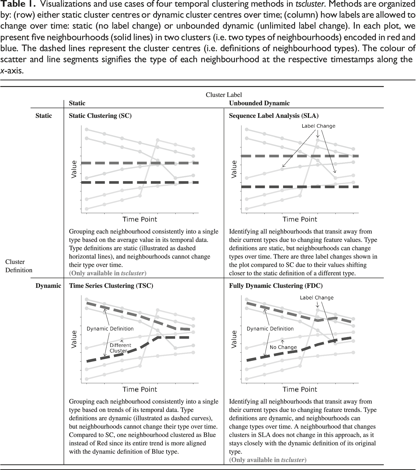
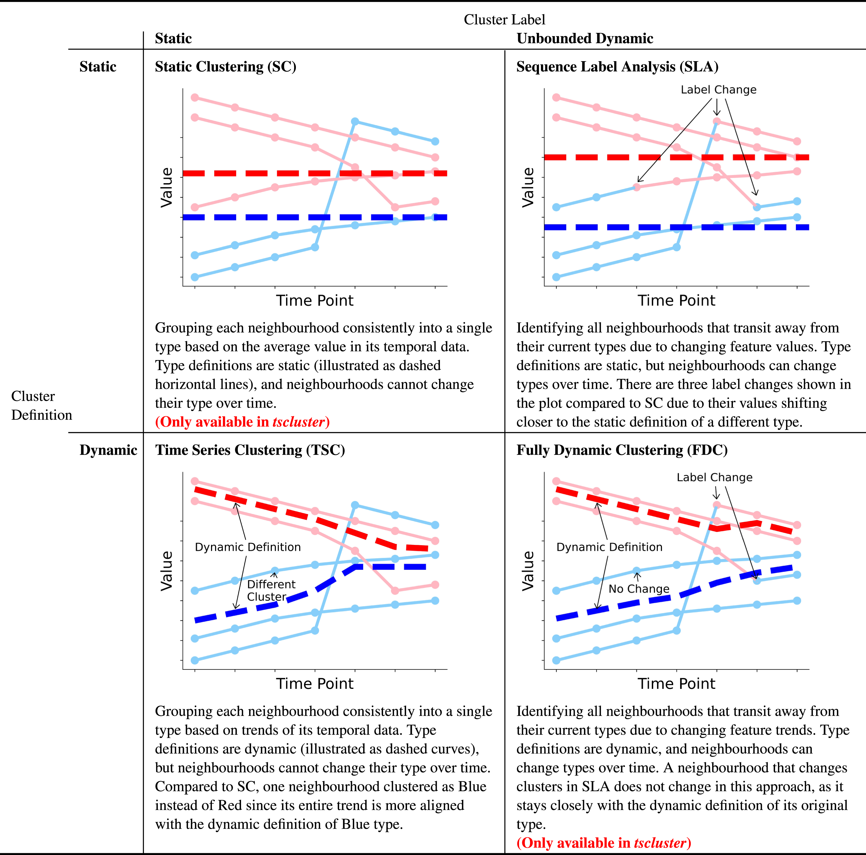
The other main technique is SLA. Several prominent studies on neighbourhood changes use a two-stage approach of temporal clustering (Cornwell, 2015; Delmelle, 2016; Dias and Silver, 2021; Kang et al., 2020), extended from sequence analysis (Aisenbrey and Fasang, 2010). The plot in the upper right of Table 1 shows an example of SLA, the first stage of this approach. In SLA, traditional clustering algorithms, such as K-means Clustering, are applied, treating each timestamp as an independent entity, allowing cluster labels to change over time while keeping cluster definitions static due to the fact that temporal relationships are being ignored. SLA tracks neighbourhood evolution by identifying changes in cluster labels, indicating transitions between types. For example, a neighbourhood might shift from ‘Residential’ to ‘Commercial’, reflecting changes in dwelling count. However, SLA’s static cluster definition is unsuitable for scenarios where the characteristics of this type will evolve over time, as the same dwelling count across years for ‘Residential’ may become unrealistic.

In addition, sequence analysis was performed in the second stage of existing studies to re-group neighbourhoods based on cluster label sequences’ similarity, measured by Optimal Matching (OM) distance (Delmelle, 2016). Kang et al. (2020) also performed a detailed sensitivity analysis of other variations of OM distance under this type of method. However, a deficiency in existing studies is the frequent use of different clustering methods than in the first stage, such as Ward’s method for Hierarchical Clustering (Ward Jr., 1963), along with different similarity measures. This discrepancy can complicate the analysis. Additionally, the use of OM distance as a sequence analysis measure remains questionable (Levine, 2000).

Depending on the specific requirements of the task at hand, either TSC or SLA might be suitable. The existing tslearn Python package (tslearn.readthedocs.io) is primarily designed for TSC, leaving a gap for applications requiring SLA. Adapting traditional clustering for SLA can be labour-intensive, often requiring repeated modifications to suit different problems. In addition, and even more importantly, there is a large and unexplored design space of temporal clustering methodologies that interpolate between the two extremes of TSC and SLA that permit novel temporal clustering approaches, like understanding neighbourhood transitions from existing temporal trends to new ones. If a unique neighbourhood initially shows a declining trend in dwelling count but has an increasing trend afterwards, it should be clustered into two different types. In this case, both cluster definition and labels are dynamic over time. A flexible temporal clustering framework is summarized in Table 1 to accommodate any combination of static or dynamic cluster definitions and labels. This framework encompasses existing approaches and bridges the gaps between them.

Another important novelty of this framework is its ability to perform bounded dynamic cluster labels (illustrated in Table 2), which introduces two additional novel temporal clustering methods with both static cluster definition (Bounded Sequence Label Analysis (BSLA)) and dynamic cluster definition (Bounded Dynamic Clustering (BDC)). These methods allow the identification of atypical time series entities by limiting the maximum cluster label changes. A potential use case in urban science is identifying neighbourhoods that change types due to external forces. For instance, an urban renewal process might shift neighbourhoods from ‘Residential’ to ‘Commercial’, reflected by atypical changes in their dwelling counts. A real-world example of identifying atypical changes using BDC can be found in the case study section.

Table 2.

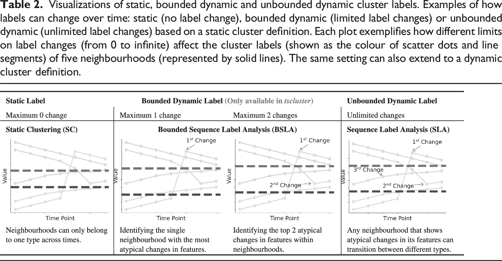
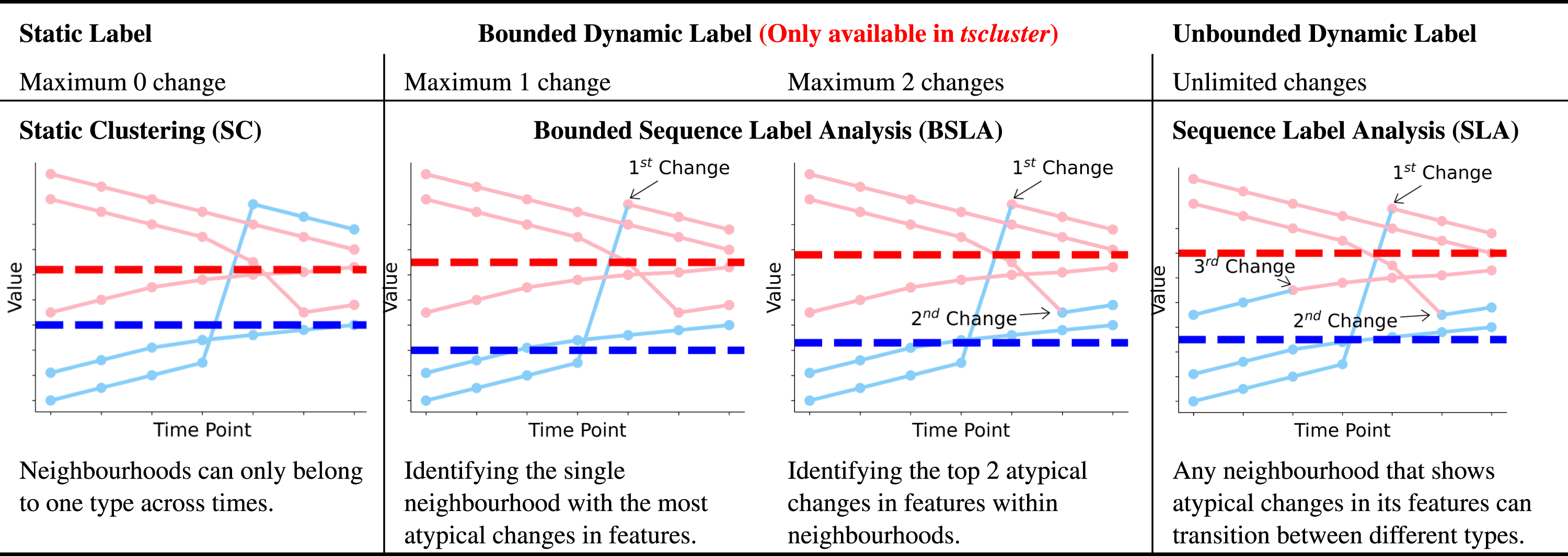
Visualizations of static, bounded dynamic and unbounded dynamic cluster labels. Examples of how labels can change over time: static (no label change), bounded dynamic (limited label changes) or unbounded dynamic (unlimited label changes) based on a static cluster definition. Each plot exemplifies how different limits on label changes (from 0 to infinite) affect the cluster labels (shown as the colour of scatter dots and line segments) of five neighbourhoods (represented by solid lines). The same setting can also extend to a dynamic cluster definition.

In addition, TSC and SLA are extensions of traditional clustering algorithms, which means they are not guaranteed to produce reproducible results and are sensitive to initialization (Celebi et al., 2013). Different initializations can potentially converge to different optimal values in the clustering objective (i.e. local minima), resulting in varying cluster definitions and labels under the same temporal data and settings. To address these issues, we introduce tscluster, a Python package that covers all the methods listed in Table 1 for temporal clustering. More importantly, tscluster utilizes mixed-integer linear programming (MILP), a type of constraint programming, to guarantee that the value of the clustering objective after optimization is globally optimal, ensuring the reproducibility of the clustering results.

Methodology

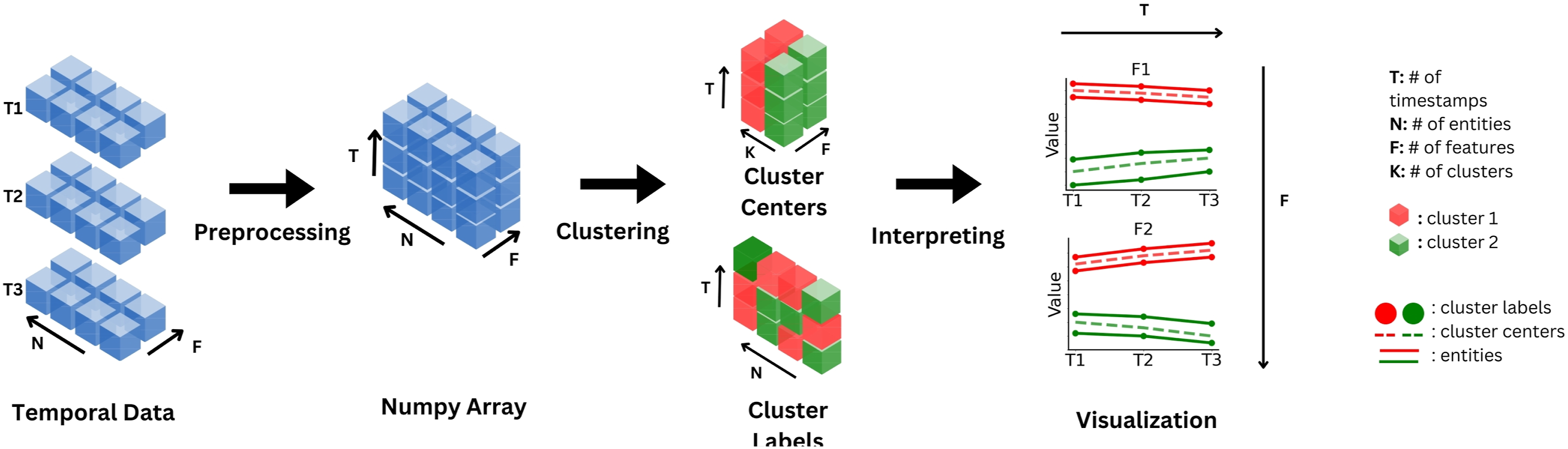
tscluster is an open-source Python package with comprehensive functionalities for temporal clustering. tscluster can be installed via PyPI (pypi.org/project/tscluster), and the source code is accessible on Github (github.com/tscluster-project/tscluster). Documentation is available online at the tscluster website (tscluster.readthedocs.io). As illustrated in Figure 1, the general temporal clustering workflow using tscluster comprises the following three steps:

1. Preprocessing: This involves manipulating the sourced temporal data, which typically includes T timestamps (e.g. years), N sociospatial entities (e.g. neighbourhoods), and F features (e.g. percent unemployed), to the required format (details discussed below). Data transformation (e.g. Z-score normalization) may also be applied to facilitate various analyses.

2. Clustering: Selecting the clustering methods with appropriate parameter settings (e.g. number of clusters K, the maximum number of clustering label changes B if selected methods allow bounded changes) from the six methods outlined in Table 1. Subsequently, the selected methods are applied to the preprocessed temporal data to derive the clustering centres and labels.

3. Interpreting Utilizing the clustering results (e.g. centres and labels) to extract insights (e.g. identifying the definition of neighbourhoods types using centres, recognizing atypical neighbourhoods that do not fit a single type based on changes in labels) from the temporal data, typically through visualization (e.g. time series plots) or numerical evaluations (e.g. total number of cluster label changes).

Figure 1.

An exemplary workflow of the tscluster package. The temporal data is preprocessed using the preprocessing sub-package into a Numpy array with dimension (number of timestamps T, number of entities N, number of features F) before applying the selected clustering methods in ‘tskmeans’ and ‘opttscluster’. The clustering result consists of K cluster definitions and T cluster labels for each entity. To interpret the result along with temporal data, the ‘tsplots’ sub-package can be used to construct visualizations, such as time series plots.

Below we elaborate on the specifics of each step within tscluster.

Preprocessing

The preprocessing sub-package loads temporal data from various formats, including Numpy Arrays, Pandas DataFrames, CSV, Excel and JSON files. Internally, as illustrated in Figure 1, the loaded temporal data was converted to a Numpy array with dimension (T, N, F), where t = 1, …, T indexes the number of timestamps, n = 1, …, N indexes the number of sociospatial entities, and f = 1, …, F indexes the number of variables or features.

The preprocessing sub-package also provides functionalities for transforming temporal data, such as Z-score normalization and min-max scaling per timestep or feature. These transformations ensure that the data is standardized and thus ready for further analysis and clustering.

Clustering

The two main sub-packages for temporal clustering within tscluster are as follows:

• tskmeans: This sub-package leverages the tslearn for TSC (Tavenard et al., 2020) and extends the K-means clustering in scikit-learn for SLA (Buitinck et al., 2013). TSC and SLA can be done using TSKmeans and TSGlobalKmeans classes, respectively.

• opttscluster: A more versatile temporal clustering that covers all methods shown in Table 1. It uses the ‘gurobipy’ (Gurobi Optimization, LLC, 2023) package to solve a MILP formulation (as shown in supplemental materials) of each temporal clustering method. The results guarantee the global optimality in the clustering objective.

Interpreting

To facilitate the interpretation of output for applied researchers, tscluster provides the tsplot sub-package to visualize temporal data and clustering results (e.g. cluster centres and labels). tsplot is capable of generating multivariate time series plots as 3-D waterfall plots for all features or separate univariate time series subplots for each feature (see Figure 2). Additionally, tscluster can numerically interpret the clustering results using two distance metrics, inertia and max distance, which are detailed in the supplemental material.

Figure 2.

The comparison between FSAs with most frequent changes – M3B from SLA (top) and M5E from BDC bottom). The solid lines are the time series of two FSAs in each feature. The dashed lines represent the centres of clusters present in M3B and M5E (i.e. three clusters in SLA and two clusters in BDC). In ‘population density’ and ‘percentage of the young population’, increases in M5E align with its cluster label changes in BDC (colour of scatter points and line segments), indicating an atypical FSA that transited to another neighbourhood type with different temporal trends in 2006.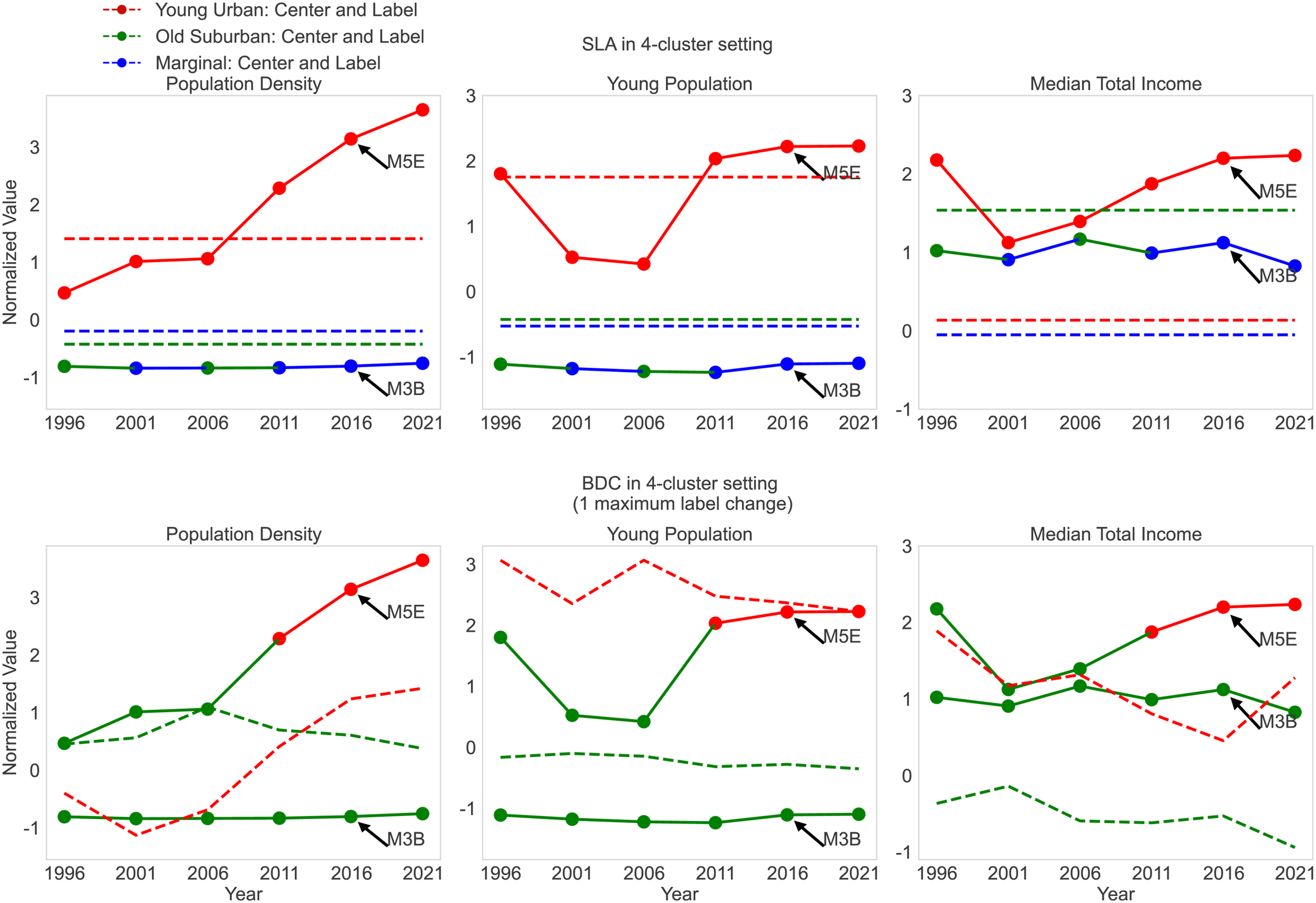

Case study

This section illustrates one use case of tscluster, showing how to apply Bounded Dynamic Clustering (BDC) to answer an important research question in neighbourhood change research: what areas of the city are the most volatile (Silver and Silva, 2021)? Specifically, we show an example of BDC in Toronto, Canada, examining F = 4 socioeconomic indicators over T = 6 timestamps from 1996 to 2021. This temporal data comes from the Census of Canada data provided by Statistics Canada via CHASS (Canada, 2021). The geographic unit for this analysis was the Forward Sortation Area (FSA), with all N = 96 entities transformed using Z-score normalization across each timestamp per feature. Further details on these features and their derivation are available in the supplemental material.

We first identified the different types of FSAs in Toronto by clustering their historical temporal data, and second, examined atypical FSAs that do not neatly fit into a single type, quantified by the frequency of label changes within each FSA. We identified four different types of FSA in Toronto and captured the FSA that exhibits the most divergent transition from one neighbourhood type to another (i.e. the most frequent changes in its cluster label).

To illustrate the distinctive capabilities of tscluster, we show both SLA with K-means clustering (i.e. TSGlobalKmeans class in tscluster), a common method for neighbourhood change analysis (Delmelle, 2016) and BDC (for this exercise, we limited the maximum number of changes to 1, where only a single FSA that least adheres to a single cluster definition will change its label). We set the total number of clusters K = 4 as determined by the Elbow method based on the ‘Within Cluster Sum of Squares’ (Nainggolan et al., 2019). This dual approach allows us to compare SLA with the novel BDC in handling temporal data for neighbourhood change analysis. The data and Python code for this case study can be found in this Colab Notebook.

Cluster definition

As depicted in Figure 1, the output of SLA and BDC consists of two main components: the static or dynamic cluster centres and a set of cluster labels assigned to each timestamp for every entity. The initial analytical step involves interrupting the cluster centre of each cluster as the specific definition for the types of the neighbourhood. To ensure consistency across the two methods, we calculate the mean of four features across all timestamps within each cluster (refer to Figure 5 and Figure 6 in supplemental materials), as well as examine their geographical distribution (see Table 2 and Table 3 in supplemental materials). Both the SLA and BDC approaches yield similar definitions for neighbourhood types, which can be summarized as follows:

1. Old Suburban: Predominantly comprising suburban FSAs concentrated within the southeast corner and midtown of Toronto with the lowest average percentage of young adults, while boasting the high average median total income.

2. Young Urban: Concentrated in the central city, this type of FSA has the highest average population density and exhibits an exceptionally high youth population. BDC further subdivided these central FSAs into an additional type, characterized by high density but a lower proportion of the younger population (termed as High-Density Urban).

3. Visual Minority: This type of suburban FSA has the highest percentage of visual minorities with the lowest median income. This cluster is situated in the peripheral regions of Toronto’s suburbs

4. Marginal: This unique type identified by SLA exhibits the lowest values across all four features and is located within Toronto’s suburbs, lacking clear geographical characteristics.

An alternative method for defining neighbourhood types in BDC entails directly utilizing the cluster centres. These centres, illustrated as dashed lines on the bottom of Figure 2, represent temporal sequences rather than static values across years in SLA (dashed lines on the top of Figure 2), allowing type definitions to temporally evolve and offering a more refined definition than static ranks when using the mean of features. Supplemental materials provide a detailed demonstration of using dynamic cluster centres as cluster definition via a case of business establishment changes in Chicago.

Atypical change analysis

To identify atypical FSAs that do not fit into a single neighbourhood type, we calculated the frequency of cluster label changes within each FSA using SLA and BDC. M3B experienced the most frequent changes in SLA, while M5E exhibited changes in BDC due to the 2000 Toronto Waterfront Revitalization Initiative (Rosen, 2017), which likely influenced population density and young professionals (Lehrer et al., 2010).

We visualized the time series of the percentage of young people and the population density in M5E and M3B along with the cluster centres and labels under SLA (left side of Figure 2) and BDC (right side of Figure 2). For M5E, significant increases in both features are observed starting in 2006, coinciding with its transition from ‘Old Suburban’ to ‘Young Urban’ under BDC.¹ However, under SLA, M5E’s cluster labels remain unchanged.

By contrast, M3B’s features do not show pronounced changes over time. However, under SLA clustering, M3B changes cluster label frequently since minor changes shift it between two nearby cluster centres (cf. Figure 7 in supplemental materials), making it susceptible to statistical noise in clustering algorithms that lack global optimality and reproducibility. Without incorporating a bound on the maximum allowable label changes (e.g. BDC) or global optimality (e.g. SLA with MILP,² entities like M3B risk transitioning repeatedly between cluster boundaries without meaningful data changes.³

This case study reveals that BDC, a novel temporal clustering method in tscluster, demonstrates significant advantages over SLA in identifying atypical FSAs. BDC successfully captures the atypical temporal behaviour of M5E, reflecting the real-world impact of the Toronto Waterfront Revitalization Initiative while avoiding misidentifying FSAs, such as M3B, located on the boundary between clusters susceptible to statistical noise. Moreover, BDC retains the ability to summarize cluster definitions similar to SLA.⁴

Conclusion

In this article, we have introduced tscluster, a novel Python package that provides a generalized framework for temporal clustering based on the dynamics of cluster centres and labels. This package offers: (1) a number of innovative techniques, such as Bounded Dynamic Clustering, that are not available in existing libraries, (2) a user-friendly interface for applying and comparing these methods, (3) globally optimal solutions for the clustering objective by employing a mixed-integer linear programming formulation, enhancing the reproducibility and robustness of the results and (4) a suite of visualization tools to facilitate the interpretation and comparison of clustering results, enabling researchers to gain deeper insights into the temporal patterns and structures within their data.

Supplemental Material

Supplemental Material - tscluster: A python package for the optimal temporal clustering framework

Supplemental Material for tscluster: A python package for the optimal temporal clustering framework in Jolomi Tosanwumi, Jiazhou Liang, Daniel Silver, Ethan Fosse and Scott Sanner by Environment and Planning B: Urban Analytics and City Science

Footnotes

Declaration of conflicting interests

The author(s) declared no potential conflicts of interest with respect to the research, authorship, and/or publication of this article.

Funding

The author(s) disclosed receipt of the following financial support for the research, authorship, and/or publication of this article: This work was supported by the Education and Training for the 21st Century Workforce (ET21) Cluster, part of the Clusters of Scholarly Prominence Program at the University of Toronto Scarborough.

ORCID iDs

Jolomi Tosanwumi

Jiazhou Liang

Data availability statement

The source code for tscluster python toolkit and the datasets and codes generated during and/or analysed in the case studies are available in the tscluster repository in Github.*

Supplemental Material

Supplemental material for this article is available online.

Notes

Jolomi Tosanwumi is a Master’s Student in Industrial Engineering at the University of Toronto. His research focuses on data science and machine learning methodologies and applications. He is currently a research assistant at Data Driven Decision Making Labs.

Jiazhou Liang is a Master’s Student in Industrial Engineering at the University of Toronto. Jiazhou’s research is focus on various range of data science applications and machine learning methodologies. He is currently a research assistant at Data Driven Decision Making Labs.

Daniel Silver is a Professor of Sociology at the University of Toronto.

Ethan Fosse is an Assistant Professor of Sociology and Associate Director of the Data Sciences Institute at the University of Toronto. He received his PhD from Harvard University and previously worked as a Postdoctoral Research Associate at Princeton University. He has published research on social change, quantitative methods, and cohort analysis in a number of journals, including Demography, Sociological Science, and the Annual Review of Sociology. He is currently working on a forthcoming book with Cambridge University Press on methods for analyzing time-series cross-sectional data.

Scott Sanner is an Associate Professor in Industrial Engineering and Cross-appointed in Computer Science at the University of Toronto. Scott’s research focuses on a broad range of AI topics spanning sequential decision-making, (conversational) recommender systems, and applications of machine/deep learning. Scott is currently an Associate Editor for ACM Transactions on Recommender Systems (TORS), the Machine Learning Journal (MLJ), and the Journal of Artificial Intelligence Research (JAIR). Scott was a corecipient of paper awards from the AI Journal (2014), Transport Research Board (2016), and CPAIOR (2018). He was a recipient of a Google Faculty Research Award in 2020 and a Visiting Researcher at Google while on sabbatical during 2022-23.

References

Aghabozorgi

Seyed Shirkhorshidi

Ying Wah

(2015) Time-series clustering–a decade review. Information Systems 53: 16–38.

Aisenbrey

Fasang

(2010) New life for old ideas: the “second wave” of sequence analysis bringing the “course” back into the life course. Sociological Methods & Research 38(3): 420–462. DOI: 10.1177/0049124109357532.

Buitinck

Louppe

Blondel

, et al. (2013) API design for machine learning software: experiences from the scikit-learn project ECML PKDD Workshop: Languages for Data Mining and Machine Learning, Prague, Czech Republic, 23-27th September, 2013, 108–122.

Canada

(2021) Census of Canada topic based tabulations, immigration and citizenship tables: immigrant status and place of birth of respondent, sex, and age groups, for population, for census metropolitan areas, tracted census agglomerations and census tracts. https://clouddc-chass-utoronto-ca.myaccess.library.utoronto.ca/census/fsa.html.

Celebi

Kingravi

Vela

(2013) A comparative study of efficient initialization methods for the k-means clustering algorithm. Expert Systems with Applications 40(1): 200–210.

Cornwell

(2015) Social sequence analysis: Methods and applications. Cambridge: Cambridge University Press, Vol. volume 37.

Delmelle

(2016) Mapping the dna of urban neighborhoods: clustering longitudinal sequences of neighborhood socioeconomic change. Annals of the Association of American Geographers 106(1): 36–56.

Dey

Rossi

Sidiropoulos

(2017) Temporal clustering. arXiv preprint arXiv:1704.05964.

Dias

Silver

(2021) Neighborhood dynamics with unharmonized longitudinal data. Geographical Analysis 53(2): 170–191.

10.

Fosse

(2023) Theorizing in the cohort mode: on ryder’s processual account of social change. Canadian Studies in Population 50(3): 5–23. DOI: 10.1007/s42650-023-00075-9.

11.

Galster

(2001) On the nature of neighbourhood. Urban Studies 38(12): 2111–2124.

12.

Gurobi Optimization, LLC (2023) Gurobi optimizer reference manual. https://www.gurobi.com.

13.

Hoai

Minh

Torre

Fernando De La

(2012) Maximum margin temporal clustering. Proceedings of the Fifteenth International Conference on Artificial Intelligence and Statistics. La Palma, Canary Islands: PMLR, 22, 520–528.

14.

Kang

Rey

Wolf

, et al. (2020) Sensitivity of sequence methods in the study of neighborhood change in the United States. Computers, Environment and Urban Systems 81: 101480.

15.

Lehrer

Keil

Kipfer

(2010) Reurbanization in Toronto: Condominium boom and social housing revitalization. disP-The Planning Review 46(180): 81–90.

16.

Levine

(2000) But what have you done for us lately? commentary on abbott and tsay. Sociological Methods & Research 29(1): 34–40.

17.

Nainggolan

Perangin-angin

Simarmata

, et al. (2019) Improved the performance of the k-means cluster using the sum of squared error (sse) optimized by using the elbow method. Journal of Physics: Conference Series 1361: 012015.

18.

Rosen

(2017) Toronto’s condo-builders: development approaches and spatial preferences. Urban Geography 38(4). https://www.tandfonline.com/doi/full/10.1080/02723638.2016.1179426?scroll=top&needAccess=true.

19.

Silver

Silva

(2021) A markov model of urban evolution: neighbourhood change as a complex process. PLoS One 16(1): e0245357.

20.

Silver

Adler

Fox

(2022) Towards a model of urban evolution—part i: context. Urban Science 6(4): 87.

21.

Tavenard

Faouzi

Vandewiele

, et al. (2020) Tslearn, a machine learning toolkit for time series data. Journal of Machine Learning Research 21(118): 1–6. https://jmlr.org/papers/v21/20-091.html.

22.

Ward

Jr (1963) Hierarchical grouping to optimize an objective function. Journal of the American Statistical Association 58(301): 236–244.

Supplementary Material

Please find the following supplemental material available below.

For Open Access articles published under a Creative Commons License, all supplemental material carries the same license as the article it is associated with.

For non-Open Access articles published, all supplemental material carries a non-exclusive license, and permission requests for re-use of supplemental material or any part of supplemental material shall be sent directly to the copyright owner as specified in the copyright notice associated with the article.

0.00 MB

27.64 MB

tscluster : A python package for the optimal temporal clustering framework

Abstract

Keywords

Introduction

Methodology

Preprocessing

Clustering

Interpreting

Case study

Cluster definition

Atypical change analysis

Conclusion

Supplemental Material

Supplemental Material - tscluster: A python package for the optimal temporal clustering framework

Footnotes

Declaration of conflicting interests

Funding

ORCID iDs

Data availability statement

Supplemental Material

Notes

References

Supplementary Material