Sage Journals: Discover world-class research

Abstract

Agent-based models are computational methods for simulating the actions and reactions of autonomous entities with the ability to capture their effects on a system through interaction rules. This study develops an agent-based simulation model (RANGE) to replicate the growth of Sydney Trains network by given exogenous historical evolution in land use. A set of locational rules has been defined to find a sequence of optimal stations from an initial seed. The model framework is an iterative process that includes five consecutive components including environment loading, measuring access, locating stations, connecting stations, and evaluating connections. In each iteration, following the locating/connecting process in each line of railways network, the accessibility will be calculated, and land use will be updated. Based on the compilation of network topology and properties, each iteration will be a year-on-year time step analysis. The network evolves based on a set of locational rules in regards to changes in the historic land use. Also, two coverage indices are defined to evaluate the fitness of the simulated lines in comparison to the Sydney tram and train network.

Keywords

agent-based model simulation accessibility railway network evolution

Introduction

Urban growth is a dynamic, complex system with many components that can be examined from various angles. The agents in this dynamic pursue their individual interests and interact with each other with some local rules. This suggests that cities are the emergent result of a self-organization process, and urban evolution is a bottom-up process and temporally dynamic (Batty et al., 2013). When considering the long-term changes of urban morphology, transport network and land use are the two main co-evolutionary subsystems (Rui et al., 2013; Wu et al., 2017).

There has been a trend towards modeling the evolution of urban areas using micro-simulation in the literature (De Martinis et al., 2014; Levinson and Huang, 2012; Rui et al., 2013; Wu et al., 2013, 2017; Xie and Levinson, 2009; Zhang and Levinson, 2017; Zhuge et al., 2016). Simulation can be an effective tool for understanding urban dynamics, and it provides planning support in managing the growth and evaluating future (or developing) scenarios. Urban dynamics have many driving forces which influence the intensity and direction of urban evolutionary processes. Central planning plays a significant role in shaping cities even if the effective time horizon of city planners and authorities is much shorter than the life-cycle of a city (Barthelemy et al., 2013). Depending on the time horizon and the level of detail, there are a wide spectrum of studies from aggregate spatial interaction models to feedback loop systems and micro-simulations used to model urban dynamics.

Transport network development is one of the main segments of urban dynamics and there has been a well-established interest in this area. Transport network development can be modeled using top-down or bottom-up mechanisms. The top-down process is when governmental authorities plan or directly impact the planning of a transport network through centralized objectives (Levinson and Huang, 2012). The bottom-up process considers local objectives that determine the decentralized and independent development of the network. In the latter mechanism, the whole network structure and its characteristics emerge from self-organization and evolution (Levinson and Huang, 2012).

For example Levinson and Yerra (2006); Yerra and Levinson (2005); Zhang and Levinson (2017) simulated the growth of road networks with investment/disinvestment rules for individual roads. The growth of transport networks is also investigated using biological phenomena since they develop without centralized control. Tero et al. (2010) compare the growth of the slime mold Physarum polycephalum with Tokyo rail system. They developed a biologically inspired mathematical model for network constructions. Sugarscape is another biologically inspired agent-based model that has been used to replicate the growth and dynamics of a system (Epstein and Axtell, 1996).

Finding the optimal configuration of a transport network is a planning and operational objective. The transport network design problem determines the configuration of the transport network, including its form and structure, with respect to a given land use and a set of constraints. The network design is a complex problem and its complexity does not permit an exact solution and requires multi-objective optimization techniques. The network design problem, specifically for the road network, is extensively discussed in the literature (Cantarella and Vitetta, 2006).

However, modeling growth and evolution of transport networks is not an optimization problem to design a better system. It aims to find a set of rules that govern the growth of a network and reflect the emergent pattern from the interactions between effective agents. Transport evolution models are critical for evaluating planning theories and future policies, particularly in the area of accessibility. An agent-based model is a micro-simulation modeling system for representing bottom-up phenomena. It can account for complex and dynamic individual behavior. This results in evolving collective patterns and self-organized characteristics.

Agent-based models are developed to simulate the behavior of individual entities interacting in heterogeneous spatial environments; once an agent-based model has been developed and validated, it can be used to gain a deeper understanding of the whole system. For instance, agent-based models have been used in simulating urban air mobility (Rothfeld et al., 2018), supply chains (Davidsson et al., 2008; De Bok and Tavasszy, 2018; Holmgren et al., 2013), service design (Rexfelt et al., 2014), and travel demand (Axhausen et al., 2016).

Agent-based models can be computationally complex and expensive, require much data, are not easily transferable and must be built as context-specific models. Because of these limits, it is important to keep the level of details low and simplify the interaction mechanisms between agents without losing the general concept. This study aims to develop a simulation framework to model the growth of a railway network using accessibility as a nexus between transport network investment and land use development.

The concept of access links transport networks and land use characteristics, but has received little attention in the evolution of transit systems. One explanation is that calculating access requires historical data and a multi-component model. The goal of this research is to develop simple rules (i.e., search, select, branch, and reconnection rules) that capture the properties of the transit network at a large scale, as well as the dynamic of transit lines and land use developments, as efficiently as possible. The Rail Agent-based Network Growth and Evolution (RANGE) model is developed to replicate growth of the Sydney Trains network as detailed in the methodology section.

Methodology

To model the growth of a railway system, initial conditions, potential station locations, potential links, connection rules, and the structural constraints must be determined. This requires taking a variety of local factors into account, including land use patterns, population and employment distribution, road networks, and topography. This is in addition to the constraints imposed by the rail transit system’s design. This section explains agent-based models, the developed simulation framework, and the parameters and constraints that are associated with an evolving network.

Agent-based model

Agent-based models are computational methods for simulating the actions and reactions of autonomous entities with the ability to capture their effects on a system through interaction rules. One of the main advantages of agent-based modeling is to enable us to have an explicit expression of feasible interaction between different and heterogeneous agents whether in a complex or a simple network. The agent-based simulation is a useful application to simulate the formation of transport networks considering individual travel behavior (Xie and Levinson, 2009).

The agent-based model evolves by itself when the initial micro-level elements (and initial conditions) have been set; macro-level characteristics emerge through an evolutionary process. Simple local rules of agent behaviors are shown to efficiently represent network demand and hierarchy in the structure of road network (Zhang and Levinson, 2004). Therefore, it is a suitable approach for our purpose to evaluate transit network evolution based on changes in land use.

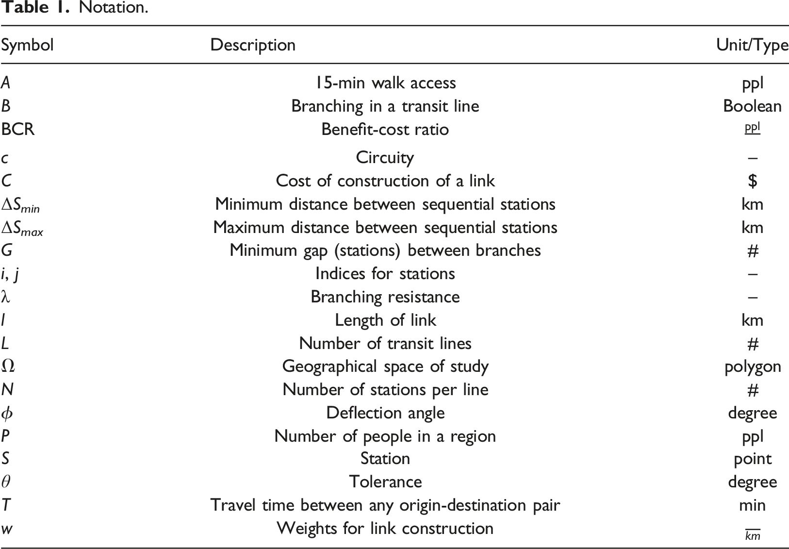
This study develops Rail Agent-based Network Growth and Evolution (RANGE) model to simulate the growth of the Sydney Trains network by using the concept of interaction between land use and transit networks. Two types of agents exist in the model including land use and transit network. The transit agent (including stations and links between them) will be generated over land use agents (the environment consists of land use parcels), and their interaction will be modeled. We use accessibility to connect land use development and transit network investment, as shown in Figure 1, which depicts a generic feedback loop between transit network and land use. In this representation, accessibility would be a surrogate measure for latent factors (Lahoorpoor, 2022b). This generic and simplified (i.e., less detailed) feedback loop reduces the computational complexity of agent interactions and requires fewer inputs. Due to the heavy computational time of the feedback, this study only models the network investment, and land use agents are passive, they change exogenously and do not evolve based on the access provided by the modeled network investment, but instead vary based on the actual conditions, presumably as a function of the historic access. Variables, parameters, and coefficients that will appear throughout this study are notated in Table 1.

Figure 1.

Interaction between land use development and transit investment. (a) Interaction decomposition. (b) Interaction positive feedback loop.

Table 1.

No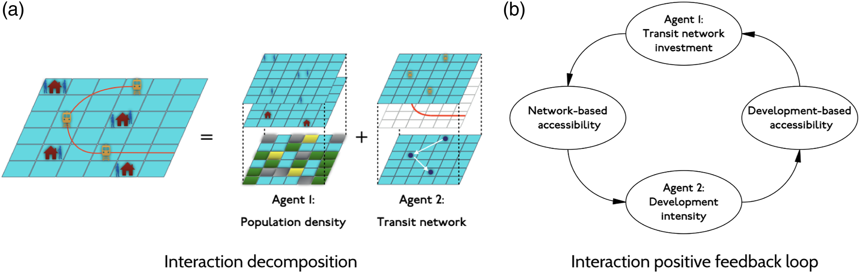tation.

Symbol	Description	Unit/Type
A	15-min walk access	ppl
B	Branching in a transit line	Boolean
BCR	Benefit-cost ratio	$\frac{ppl}{$}$
c	Circuity	–
C	Cost of construction of a link	$
ΔS_min	Minimum distance between sequential stations	km
ΔS_max	Maximum distance between sequential stations	km
G	Minimum gap (stations) between branches	#
i, j	Indices for stations	–
λ	Branching resistance	–
l	Length of link	km
L	Number of transit lines	#
Ω	Geographical space of study	polygon
N	Number of stations per line	#
ϕ	Deflection angle	degree
P	Number of people in a region	ppl
S	Station	point
θ	Tolerance	degree
T	Travel time between any origin-destination pair	min
w	Weights for link construction	$\frac{$}{k m}$

Simulation framework

In an evolutionary process, a simulation framework is developed to replicate the growth of a railway network by given exogenous historical evolution in land use. Figure 2 illustrates the flowchart of the proposed model and the architecture of agents. As a whole, the co-evolution of land use and railways network is represented as an iterative process that includes six consecutive components: exogenous land use and road network loading and setting up initial parameters, measuring walking access, locating stations, connecting stations, evaluating connections, and evaluating network circuity, which will be explained in turn. In each iteration, following the locating/connecting process in each line of railways network, the land use will be updated and walking access will be calculated. Based on the compilation of network topology and properties, each iteration will be a year-on-year time step analysis.

Figure 2.

Model’s flowchart and agents architecture: Agent 1 is the transit network which has stations and links. Agent 2 is the land use layer which includes the population and land characteristics.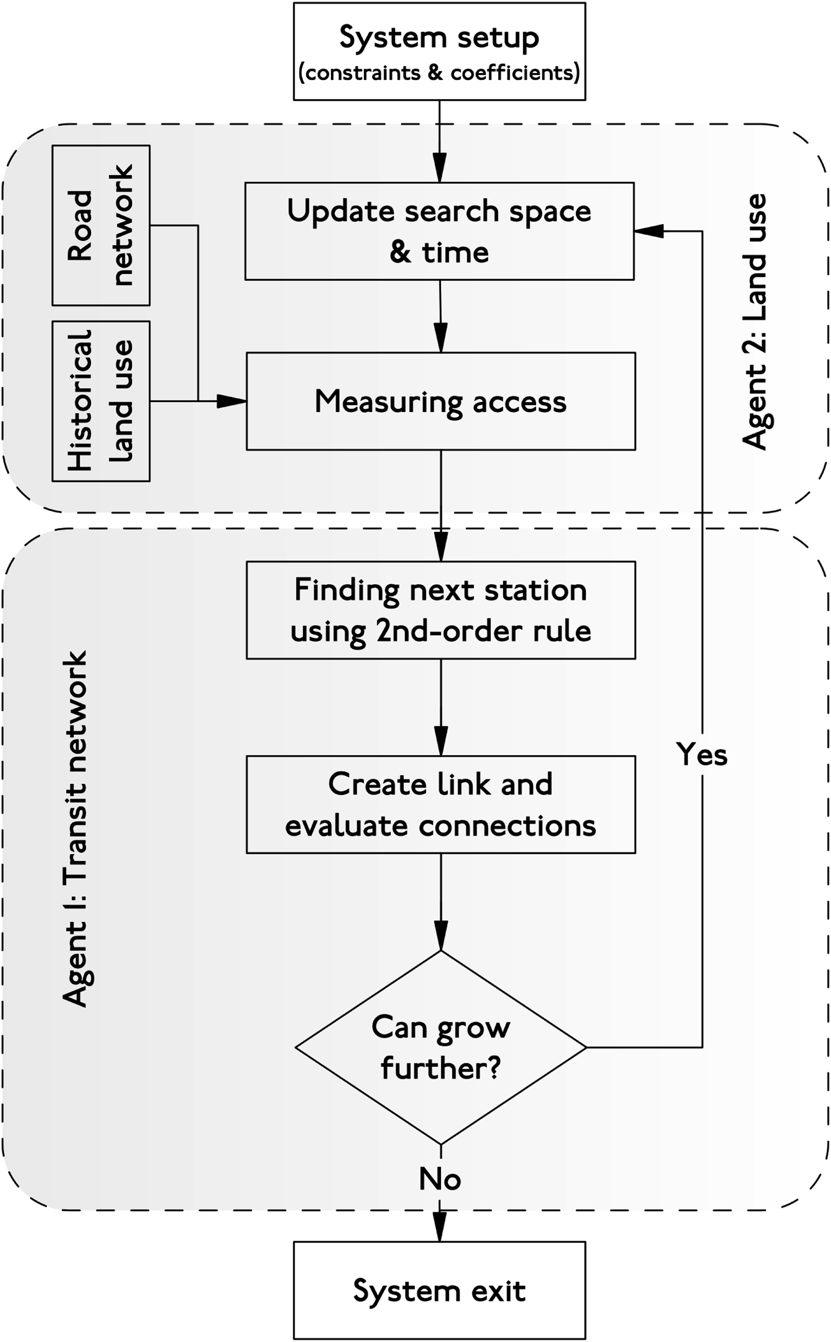

As mentioned previously, the system contains two distinct types of agents;

The transit network is the first agent. This agent type corresponds to a train line consisting of stations (i.e., nodes) and track (i.e., links) that connect them. A transit line’s (or transit agent’s) behavior is to extend its coverage and maximize its potential ridership. In each time step, the transit agent seeks the next best station given the constraints defined. Transit agents can compete, but they can share stations and create transfers during the development process. The line can be extended from the terminal and any potential transfer stations (the emergence of transfer stations is discussed in the following subsections). Each transit agent has a set of bi-directional links with the sequence of stations, and they can determine whether or not to expand based on the potential link’s length and associated costs.

The second agent is the land use agent, which corresponds to land parcels. Land use agents contain information on population, proximity to transit stations, and access to other locations. The population is externally updated at each time step, and each agent can assess the locational walking accessibility of a given road network. Each land use agent is able to detect the presence of a train station on itself or in neighboring cells. This study does not utilize regional access by transit (access based on development in Figure 1).

Each time step, transit agents observe their environment, interact with parcels within their search space, and obtain the locational walking access measures. If the network decides to expand, it makes a connection between the next potential station and the terminal (or transfer station) and evaluates the network’s characteristics as described in the subsections below. The development rate in this study is one link per year.

Search space and local search rules

The search space for locating stations depends on the study area and the land use characteristics. The study area is divided into smaller cells (which do not necessarily have to be the same size) and the feasibility of each cell as a potential station is evaluated based on land use and planning requirements (Ahmed et al., 2020).

For the case of Sydney, the study area will be divided into approximately 59,000 meshblocks (approximately city blocks, as defined by the Australian Bureau of Statistics (ABS) for the year 2016, typically associated with 30 to 60 single-family dwellings in suburban areas). The reason is twofold. First, meshblocks have scale (i.e., the more developed an area is, the smaller the blocks are) and reflect the historical land development characteristics. Using today’s meshblocks carries an exogenous and predefined land use attraction (where places get developed more) into the input dataset. Second, it helps to reduce the size of the search space in the areas that are on the outskirts of the city center.

Based on planning requirements, exclusion criteria for a site location include being in national parks, flood plains, rivers, or heritage lands. These criteria are used to filter the search space. The search space can be written as equation (1)

Ω_{f} = Ω_{m} - Ω_{e}

(1)

where Ω_f is the set of feasible blocks, Ω_m is the set of all study area meshblocks, and Ω_e is the set of excluded blocks.

In order to select the next stations, a local rule is defined to identify a series of potential locations around the initial station (or the last station in the previous growth stage). The potential locations should not be too close or too far from the previous station. Therefore, a minimum and a maximum distance between two successive stations are defined to form a “Goldilocks” zone. The potential stations are the land parcels (meshblocks) within the Goldilocks zone as depicted in Figure 3(a) and formulated in equation (2)

S_{J} \in Ω_{f} : Δ S_{\min} \leq l_{S_{i} - S_{j}} \leq Δ S_{\max}

(2)

where S_J is the selection set of potential locations of station j.

l_{S_{i} - S_{j}}

is the distance between the potential station j and the initial/previous station i. ΔS_min and ΔS_max are the minimum and maximum distance between two successive stations, respectively.

Figure 3.

Goldilocks zone and selection criteria. ΔS_min and ΔS_max are minimum and maximum distance between two successive stations, respectively. (a) First-order Goldilocks zone. (b) Second-order Goldilocks zone.

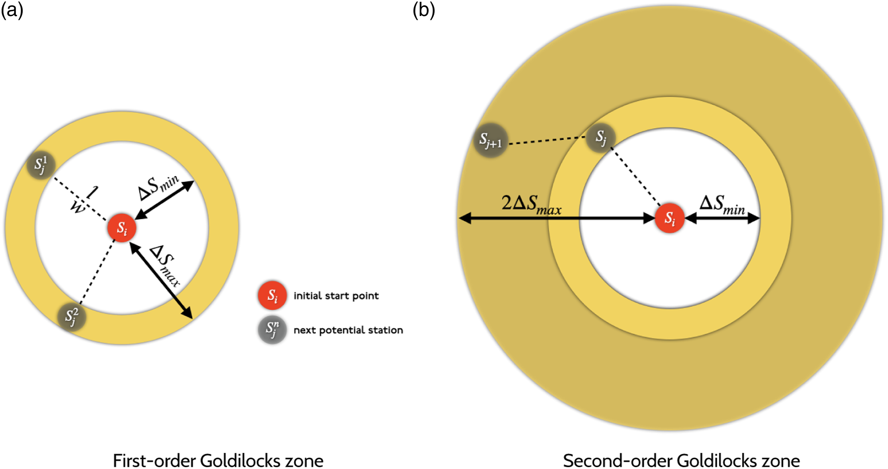
In a series of station selections, two stations should not be too close to each other. Therefore, the blocks that are within the ΔS_min of stations will be excluded from the search space in the next iterations (we name it as deactivation stage), except for transfer stations where a reconnection pattern is defined. This minimizes the choice set and expedites the running time.

One method to improve locating the next station is to look one step ahead. The second-order selection rule states that the search space would include all points in the initial station’s Goldilocks zone as well as all other points’ Goldilocks zones. For determining the next station from the selection set, a greedy heuristic algorithm is used to maximize the total benefit-cost ratio as formulated in equation (3). Access is a surrogate measure for potential ridership and revenue. The second-order search space is illustrated in Figure 3(b)

Maximum BCR = \sum \frac{Benefit}{Cost} = \sum \frac{A_{S_{j}}}{C_{S_{i} - S_{j}}}

(3)

A_{S_{j}}

is the 15-min walking access (cumulative opportunities) from S_j as equation (4)

A_{S_{j}} = \sum_{n = 1}^{N} P_{n} \cdot f (T_{S_{j} - n})

(4)

f (T_{S_{j} - n}) = {\begin{cases} 1 & if T_{S_{j} - n} \leq 15 \min \\ 0 & otherwise \end{cases}

where P_n is number of people living/working on cell n.

T_{S_{j} - n}

is travel time between station j and cell n.

f (T_{S_{j} - n})

is the impedance function.

And $C_{S_{i} - S_{j}}$ is the construction cost of link S_i − S_j based on its length, weight, and angle of deflection as illustrated in equation (5)

C_{S_{i} - S_{j}} = w_{S_{i} - S_{j}} \cdot l_{S_{i} - S_{j}} \cdot f (ϕ_{j})

(5)

where

l_{S_{i} - S_{j}}

is the length, and

w_{S_{i} - S_{j}}

is the weight of link between station i and j. The weight is determined by the topology of the study area. f (ϕ_j) is an impedance function to reflect the cost of deviation from the previous link’s direction.

Estimating the travel time is essential in the calculation of the accessibility measure. Generally, the travel time of an origin-destination pair is taken to be the minimum time one can travel the shortest path found in the network between two points of interest by walking. The travel time between the potential location and surrounding blocks is calculated using the open-source platform OpenTripPlanner V1.3.0. The walking speed is set to be 4.8 km/h (3 miles per hour). Due to the lack of historical data about roads’ opening and closure dates, the available pedestrian network is assumed to be fixed and equal to the existing (2021) network. It is worth noting that, using the 2021 road network will have little effect on locational accessibility because, historically, people tend to cluster around available roads. We therefore hope that the historical changes in land use will prevent the overestimation of access.

Branching and reconnection rules

A connection rule is defined to simulate the emergence of transfer stations in a growing network. This branching rule allows another transit line to start to grow from a junction point. A criterion is defined as whether a transit line should branch at a particular station. We assume that if the benefit-cost ratio of the following potential station is less than the second-best option of all the stations excluding adjacent to previous transfer stations (this is controlled by transfer gap parameter which will be discussed in the following subsection), then a branch occurs at the station with the previous second-best potential station. A branching resistance factor is defined to reflect the reluctance of constructing a new line (i.e., the junction cost). The branching is represented as a Boolean variable in equation (6)

B = {\begin{cases} True & if λ \cdot {BCR}_{j + 1} < {BCR}_{j}^{2 n d} : \forall j \in J - {i \pm G} \\ False & otherwise \end{cases}

(6)

where λ is the branching resistance factor, BCR is the benefit-cost ratio of stations, and G_i is the minimum gap between transfer station i in a transit line.

With the rules that have been established by now, a transit line can grow from an initial seed, extend in space, and branch off into other lines with respect to constraints and exogenous variables. However, these rules give the network a tree pattern structure. The network’s closest branches should interconnect to form loops. Consequently, a reconnection behavior is modeled in order to connect transit lines and increase the number of transfers. In the developing stage, when a line is expanding from one of its ends and finds an existing station (built in the preceding stages) around itself with an angle within a certain range, it connects to the station and forms a junction with the other line. Limiting the junction angle to ±45° eliminates semi-parallel connections and permits perpendicular-like junctions.

Constraints

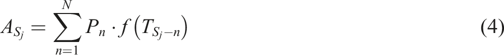
Number of lines and stations per line

The number of lines and the number of stations in the system are two main constraints in the simulation. These two variables determine the network’s potential size. The number of transit lines (L) shows how dispersed the network can be. The number of stations per line (N) indicates how far the network can be extended and is proportional to network diameter. Given a fixed number of stations in a system and a confined urban space, the network pattern would be radial if the number of stations per line increases (i.e., the number of lines decreases). In contrast, the network would have a tree-like structure as the number of stations per line decreases. These constraints are relaxed in most of the simulation runs to be an emergent property of the model.

Start point and start direction

The location of the first station of a train line, as well as the direction in which it will develop, are the critical initial parameters that affect the trend of growth. Existing train lines and historical data can be used to calibrate these parameters when simulating the growth of a network. However, they can be used to evaluate other alternatives and scenarios (for example, what if the network initially expands towards the north-east?).

Sequence of growth

Based on the number of lines, the sequence of their growth can lead to different configurations. The sequence of growth can be categorized into two types. First, the growth of lines occurs in order, that is, the second line begins to develop once the first line is completed. The second type of growth occurs when all the lines grow simultaneously. The difference is that some lines may compete with each other to find the best next station in simultaneous growth. A combination of these two types is also possible, but it is beyond the scope of this research. In this study, transit lines compete with each other, and the best station from all the potential candidates is selected to expand the network (i.e., one station per iteration, or “year”).

Line angle variation

The angle of deflection from the initial (previous) growth direction is another parameter that affects finding the next station. Expansion of a line is usually limited to one direction (e.g., east-west, north-south, etc.) to avoid unusual zigzags and U-turn growth. However, dis-alignment is possible when the benefit outweighs the cost (or no other option exists). In order to consider this constraint, the angle of deviation impacts the cost of the potential link via an impedance function, as in equation (7)

f (ϕ) = {⌈ \frac{ϕ}{θ} ⌉}^{2}

(7)

where ϕ is the deflection angle between two segments (Figure 4) and θ is the tolerance.

Number of transfers

The purpose of the branching rule is to locate intersections along a transit line. However, these points should not necessarily be consecutive, and the emergence of transfer stations should be constrained by a minimum distance (or number of stations) between them. As a result, a constraint is defined to allow testing scenarios where two adjacent stations do not become transfer points on a line.

Circuity of transit lines

Spiraling is a possible behavior of an evolving transit line. To avoid open-loop growth, the measure of circuity is used to evaluate the network’s growth. Circuity is defined as the ratio of network distance to Euclidean distance between two points (Levinson and El-Geneidy, 2009) as mathematically expressed in equation (8). In this study, the circuity is measured between all stations and the initial start point. A threshold (k) is defined to prevent the line from growing if one of its ends exceeds the threshold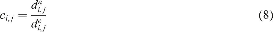

c_{i, j} = \frac{d_{i, j}^{n}}{d_{i, j}^{e}}

(8)

where c is circuity between point i and point j,

d_{i, j}^{n}

is the network distance, and

d_{i, j}^{e}

is the Euclidean distance.

Summary of the system and performance measures

A set of rules is defined that govern the evolution of a transit system (in this case, a railway). Once the initial seed is set, the first step is to locate the potential stations from the initial seed (or the end points of lines in the next stages). The second step is to choose the best station system-wide (among lines’ candidates) to connect to network. The third step is to evaluate the structure to locate possible transfer stations (a junction point where another line can emerge or two lines reconnect) and to satisfy system constraints.

If the growth of a line from one end exceeds the circuity to the start point, the line’s growth from that end is disabled. After the expansion stage is complete, the land use is updated, and the process is repeated. The model is terminated when no alternative is discovered during the searching stage. At the end of each simulation step, a series of topological measures are computed to evaluate the collective structural features of the emergent network from different dimensions, including network length, network diameter, meshedness, centrality measures, and the gamma index (γ).

Figure 4.

Deflection angle between two line segments. The angle ranges between 0 and 180°.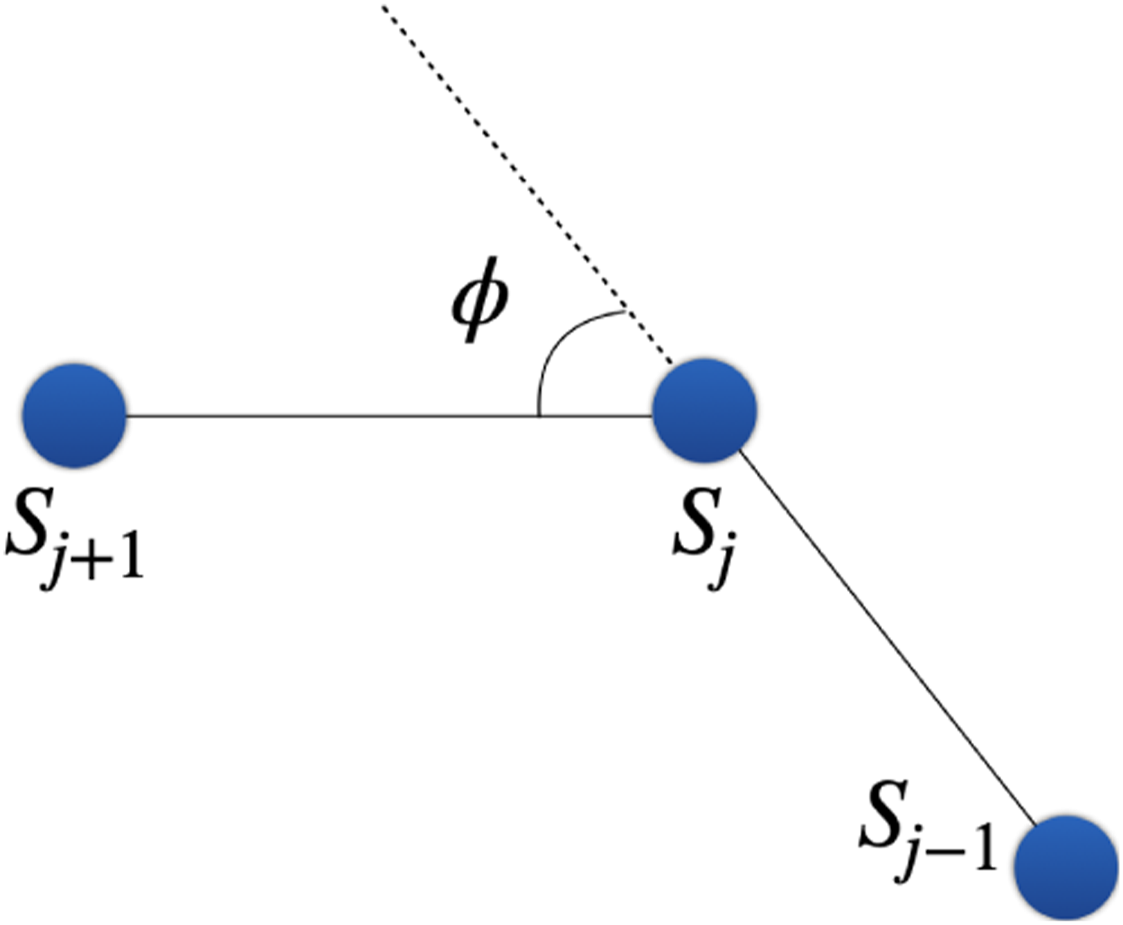

The model RANGE is written in Python 3.9 (Lahoorpoor, 2022a), and the outputs are visualized in QGIS 3.22.

Case study

Sydney, Australia, with its extensive public transport, serves as the case study. Sydney’s train network is the backbone of public transport in the inner (with a central underground core) and middle suburbs that covers over 815 km of track serving 178 stations over nine service lines.¹ In 2016, the Sydney Trains network accounts for more than 16% mode share of journeys to work (ABS, 2016, Charting Transport, 2017). The network initially evolved between Sydney and Parramatta (from Redfern to Granville station) and continues to grow to this day, with a recent Metro line opening in 2019, and extensions under construction and planned. The location of stops, stations, platforms and also, road and walking networks outside the stations were collected from the OpenStreetMap database. Figure 5 illustrates Sydney Trains network.

Figure 5.

Sydney Trains network (2021). Redfern-Central and Granville stations were the first built stations in Sydney. Basemap: OpenStreetMap.

Simulation experiments

As previously described, a simulation framework is developed to simulate the growth of a train network in the presence of exogenous land use. Numerous simulation experiments have been conducted to evaluate the model. To investigate the behavior of the system and the effects of defined parameters, 15 sets of simulation runs are defined according to the possible variable combinations. Most of simulation tests use historical land use data for Sydney, and the system runs on a year-by-year time steps (from 1851 until 2016). Because the number of possible time steps is roughly equal to the number of Sydney train stations, the development rate has been set at one station per year. Table 2 summarizes the experiments conducted in this study.

Table 2.

Simulation runs.

Sets	Algorithm	Initial point	Initial direction	Goldilocks diameter (km)	Parameters	Objective access
Set_1		Varying	Varying	1–1.5	Varying	Historical pop
Set_2		Redfern	220°–40°	1–1.5
Set_3	Transfer w/o	Central	220°–40°	1–1.5	Branching [1,2,5,10]
Set_4	reconnection	Central	245°—65°	1–1.5	Transfer gap [1—10]	Historical pop
Set_5		Redfern	245°—65°	1–1.5	Circuity [1.3, 1.5, 1.7, 1.9]
Set_6		Central	220°–40°	1.5—3
Set_7		Redfern	220°–40°	1–1.5
Set_8	Transfer w/	Central	220°–40°	1–1.5	Branching [1,2,5,10]
Set_9	reconnection	Central	245°—65°	1–1.5	Transfer gap [1—10]	Historical pop
Set_10		Redfern	245°—65°	1–1.5	Circuity [1.3, 1.5, 1.7, 1.9]
Set_11		Central	220°–40°	1.5—3
Set_12		Central	220°–40°	1–1.5	Branching [1,2,5,10]	2016 (pop + job)
Set_13	Transfer w/	Central	220°–40°	1–1.5	Transfer gap [1—10]	Historical (1pop + 2job)
Set_14	reconnection	Central	220°–40°	1–1.5	Circuity [1.3, 1.5, 1.7, 1.9]	Historical (2pop + 1job)
Set_15		Central	220°–40°	1–1.5		Historical (1pop + 1job)

Validation

The following subsections describe a series of experiments in simulation Set 1 to investigate the role of different constraints. Detailed results are provided in Supplementary Material.

Initial seeds and directions

The initial seeds of growth have a significant impact on the network’s form, shape, and structure. To determine how these initial conditions affect the results, two stations were chosen and the growth of a single line in various directions was simulated. The results indicate that by including an impedance function in the network evolution model, the network grows in a stable direction. Additionally, some initial directions result in simulated lines that closely resemble the actual network.

Number of lines and stations

As previously stated, one of the constraints that impacts network expansion and diameter is the number of stations and lines. Numerous combinations of these two constraints are feasible (different lines and different stations per line). With fixed initial seeds (i.e., initial station and initial direction), several lines with varying number of stations were simulated without using the branching mechanism discussed in the following section. The results indicate that in some lines with a relaxed station count, the line expands to a fixed point due to a lack of alternative routes. Along rivers, bays, and national parks, this occurs. With a large number of stations, a line is capable of spinning in circles, especially as access to the outer suburbs decreases.

Branching mechanism

A transfer station is an emerging property to the growth of a transit system. A connection rule is defined to determine whether a line can have a branch. The branching resistance is one variable that has an effect on the branching mechanism (which reflects the junction cost). The model is tested for four resistance values (λ = 1, 2, 5, 10) to determine the effect of branching resistance. The results indicate that when branching resistance is low, the network branches rapidly during the early stages of growth, particularly in the vicinity of central districts. Therefore, the network tends to be radial from the center. As resistance increases, the total number of lines decreases and more loops appear at the ends of lines, especially in low-density areas.

Evaluation

In order to validate the simulation results with the reality, two coverage indices are defined to evaluate the close between the simulated network and the existing lines. The first coverage index is the ratio of simulated stations within a distance of existing stations, and the second index is the ratio of simulated stations within a distance of existing lines. These measures are defined as equations (9) and (10)

{Coverage}_{1} = \frac{Number of simulated stations within existing stations buffer}{Number of expected stations} = \frac{| V_{w, s}^{d} |}{| V_{E} |}

(9)

{Coverage}_{2} = \frac{Number of simulated stations within existing lines buffer}{Number of expected stations} = \frac{| V_{w, l}^{d} |}{| V_{E} |}

(10)

Results

A series of local rules are defined to simulate the evolution of railways in a bottom-up process. More than 2000 scenarios are tested, and the fitness of simulated lines is evaluated. We observed some of the simulation lines resemble historical tram lines. The Sydney tram was born in 1879, reached its maximum extent (more than 290 km) around 1925, and was completely removed by 1961. Several segments of the tram network were integrated with the train system, and buses replaced a significant portion of the tram network. In 1997, the tram network was reborn as a modern light rail system (LRT) (Lahoorpoor and Levinson, 2022). Therefore, the coverage indices are measured for two systems: (a) existing train lines only; and (b) the 1925 trams and train network. In order to find the best answers, three buffer radii are used to evaluate the simulation runs. The evaluation results are depicted in Figure 6.

Figure 6.

The coverage ratio for simulation Set_15. The size of the dots corresponds to the relative coverage ratio. (a) Train Coverage_1. (b) Train Coverage_2. (c) Tram and Train Coverage_1. (d) Tram and Train Coverage_2.

The coverage results indicate that, not surprisingly, with higher buffer radii, the coverage ratio increases. This is because more simulated stations are within the large coverage area. Also, higher circuity (relaxing the spiraling of the network) leads to better results in some scenarios.

The results of Tram and Train Coverage_2 for a 400 m buffer indicate that the branching resistance λ = 1, circuity c = 1.9, and transfer gap G = 7 have the highest coverage ratio. Figure 7 illustrates the evolution of the network for these parameters. As seen from the figures, the network expands from Central Station and branches out with multiple lines, becoming interconnected as transit lines rejoin in further development steps.

Figure 7.

Simulation Set_15 result from Central Station with branching resistance λ = 1, circuity c = 1.9, and transfer gap G = 7. (a) 1851. (b) 1861. (c) 1881. (d) 1921. (e) 2001.

During the evolution of a simulated transit system, network characteristics are evaluated. Figure 8 illustrates the temporal changes of various attributes, such as network diameter, the total length, average link length, average centrality measures, and the meshedness of the network. In terms of diameter, both simulation and observation reach to more than 50 links. The historical trend of meshedness is different. In the simulation, reconnections are rare, whereas the number of loops is greater in reality. In addition, as a result of the historical closure of some lines and segments in Sydney Trains, the meshedness pattern exhibits more jumps.

Figure 8.

Network characteristics of the simulated system: Simulation Set_15 result from Central Station with branching resistance λ = 1, circuity c = 1.9, and transfer gap G = 7. (a) Diameter and meshedness. (b) Total and average link lengths. (c) Closeness and betweenness centrality.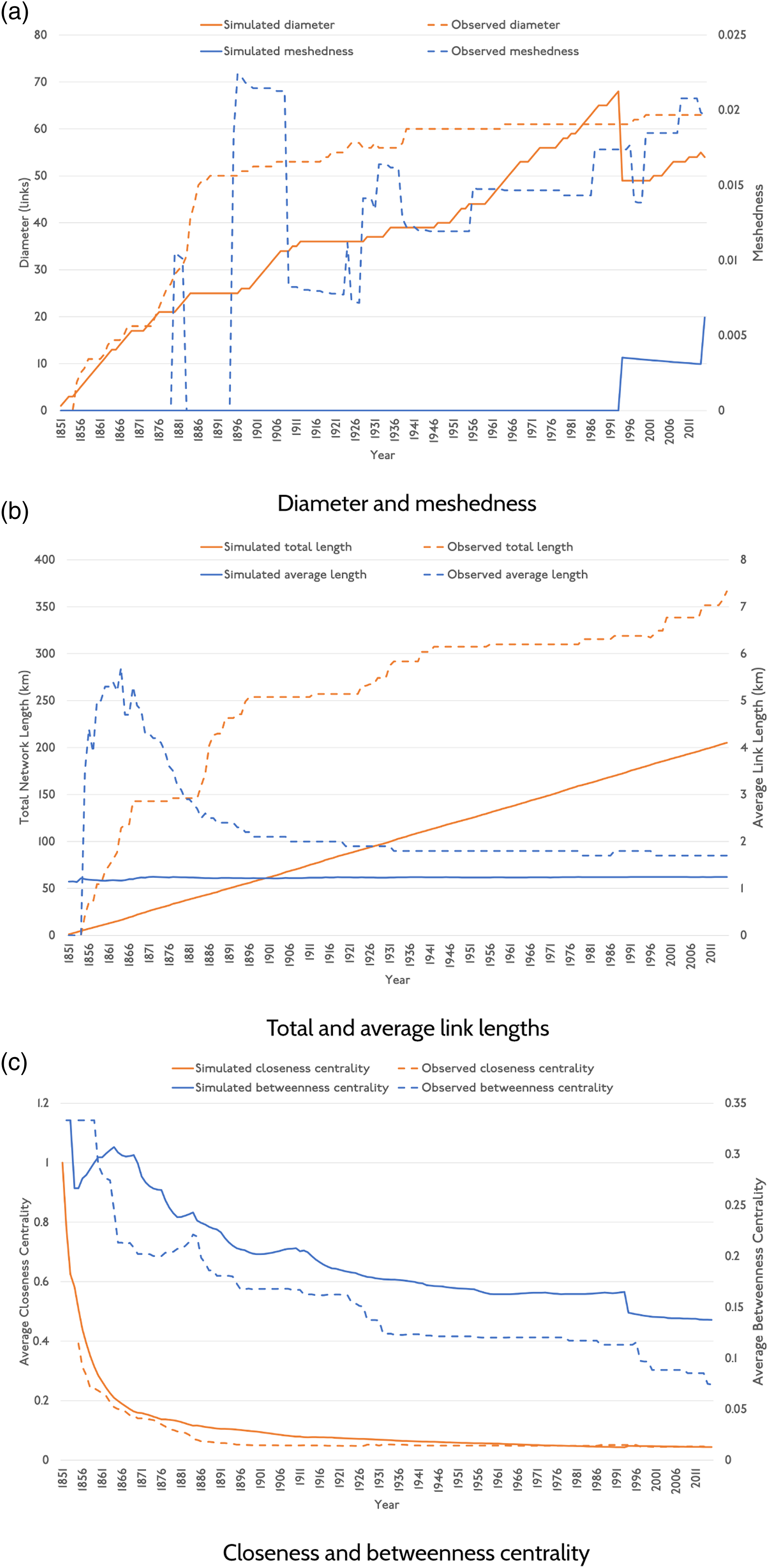

The results indicate that the network continues to expand to a total length of over 200 km and that the average link length converges to 1.24 km. Historical observation of Sydney Trains indicates a different average link length pattern because of in-fill stations. The network grew by more than 350 km, which reflects the intercity connectivity of the system.

The observed and simulated measures of closeness centrality follow the same pattern and eventually converge to the same value. The betweenness centrality measures decrease over time, but the simulated network has a greater betweenness due to fewer loops and alternative shortest paths.

Conclusion

The emergent properties of evolutionary systems can be modeled a bottom-up process using an agent-based model. Within the context of urban dynamic systems, agents can represent land parcels and transit networks. By simulating their behaviors and interactions, the model can reveal how the transit system evolves and how it responds to changes in land use.

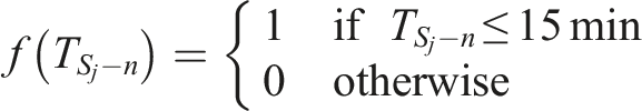
This study develops an agent-based simulation framework for modeling the growth of Sydney’s train network. In an evolutionary setting, a set of locational rules has been defined to find locally optimal stations from an initial seed. A second-order search space is used to improve the selection criteria for the next moves. Additionally, an impedance function is used to reflect the costs associated with unwanted deviations (zigzags) in a line’s growth. The model calculates the accessibility of 15 min walking from potential stations as a surrogate for the benefits and selects the locations with the highest benefit-cost ratio evaluated locally. To model transfer stations as an emergent property of network growth, a branching mechanism is developed. Therefore, the network evolves in response to changes in historical land use, based on a set of locational rules.

Furthermore, to expedite finding local solutions, this study defined a deactivation rule for excluding the cells (in the search space) that already have access to stations. Also, when two lines want to intersect or when two of their stations are close together, a re-joining connection rule is defined to improve the performance of the simulation model. This can be a way to model the advantage in increasing the regional accessibility rather than simply walk access to stations.

Fifteen distinct sets of simulation experiments were carried out to evaluate the possible combination of the constraints and parameters. The results indicate that simulating lines using predefined initial seeds can result in simulated lines that are more closely aligned to the existing network. The second set of experiments defines only one initial location and leaves branching to the system’s branching mechanism. The results indicate that by adjusting simple local rules, the model can be used to replicate the growth of train lines. Furthermore, the results suggest that, through the implemented framework, the concept of “access” can be employed as a localized search target, without having a system-wide perspective. This implies that in the assessment of proposals for transport development, a significant portion of decision-making may have been (subconsciously) influenced by the objective of optimizing access, as evidenced in the early stages of the London Tube proposals (Levinson et al., 2016).

There are a few theoretical points that must be addressed. First, the constraints serve to regulate the behavior of the agent-based model. For example, the deviation cost does not pertain to operational expenses. It is due to the design logic of railway construction and to eliminate zigzags. The other topic of debate is the interpretability of the low-level interaction constraints within the model’s global perspective. The parameters and constraints defined control the model’s behavior in order to calibrate it for a particular case study, different cases may yield alternative better fitting constraint values (see Supplementary Material).

Second, the model should take the presence of other networks (trams, for example) into account. Because, some of the simulated lines replicate tram lines and it is worth noting that the train network may have competed with the tram system since there were several proposed train lines either along the tram lines or had converted to tram lines. Third, the calibration of the variables and associated coefficients will require additional simulation experiments.

The land use agent in this study was passive and changed endogenously. Modeling the complete feedback loop (i.e., making the land use agent active and dynamic) where regional access by transit modifies land use patterns will be a worthwhile future research direction. Also, the assumption of linear development speed (one station per time step) can be improved by more sophisticated models that determine the speed of development endogenously, where construction costs rose with the number of lines being constructed simultaneously. Also, the Goldilocks zone logic implies contiguous station development rather than the construction of a long-distance line with infill development planned for later stages. Defining a variable minimum distance between stations (i.e,. initially longer distances and shorter distances subsequently) and using higher-order search rules may enhance the temporal replication accuracy of the model during the growth and early stages of development. However, this would increase computational costs and add complexity to other model components.

The primary objective of this study was to replicate the historical growth of the railway network by utilizing locational access as a surrogate to optimize network ridership. However, it is important to acknowledge that when aiming for replication, there is a risk of overfitting, which could potentially undermine the applicability of the simulation model. To address this concern and enhance the utility of the model for future planning and decision-making, future research should include a comparative analysis to evaluate the predictive accuracy of the model. This would involve assessing how well the model predicts future growth by comparing its projections with the actual developments that occurred at different points in time. Furthermore, for practical planning and strategic decision-making processes, incorporating system-wide access considerations into the objective function offers a more comprehensive perspective. This expansion of the model’s focus would enable a better understanding of the broader impacts and implications of network changes.

It is important to point out that the model could be applied to any idealized environment with a variety of different structures. The proposed model (by altering the exogenous inputs) can also be used to simulate the evolution of train network in other cities (e.g., state capitals in Australia) with train systems. This will enable us to compare how different urban topographies, different land use data, and initial seeds affect the evolution of railways. Numerous additional experiments can be conducted, as any combination of initial conditions is possible.

Supplemental Material

Supplemental Material - An agent-based simulation model for the growth of the Sydney Trains network

Supplemental Material for An agent-based simulation model for the growth of the Sydney Trains network by Bahman Lahoorpoor and David M Levinson in Environment and Planning B: Urban Analytics and City Science.

Footnotes

Declaration of conflicting interests

The author(s) declared no potential conflicts of interest with respect to the research, authorship, and/or publication of this article.

Funding

The author(s) received no financial support for the research, authorship, and/or publication of this article.

ORCID iDs

Bahman Lahoorpoor

David M. Levinson

Supplemental Material

Supplemental material for this article is available online.

Note

Bahman Lahoorpoor holds PhD in Transportation Engineering from the University of Sydney. His research interests include Transport and Land Use Interaction Models, Network Econometric Models, Network Evolution, and Urban Accessibility.

David M Levinson is a transport professor. He researches Accessibility, Transport Economics, Transport Network Evolution, and Transport and Land Use Interaction. He is the author of several books including The Transportation Experience, Planning for Place and Plexus, A Political Economy of Access, Elements of Access, and The End of Traffic and the Future of Access. He blogs at http://transportist.org.

References

ABS (2016) Australian Bureau of Statistics. Canberra, Australia: ABS, 161.

Ahmed

Nur

Ochieng

(2020) GIS and genetic algorithm based integrated optimization for rail transit system planning. Journal of Rail Transport Planning & Management 16: 100222.

Axhausen

Horni

Nagel

(2016) The Multi-Agent Transport Simulation MATSim. London: Ubiquity Press.

Barthelemy

Bordin

Berestycki

, et al. (2013) Self-organization versus top-down planning in the evolution of a city. Scientific Reports 3: 2153.

Batty

Vargas

Smith

, et al. (2013) SIMULACRA: fast land-use—transportation models for the rapid assessment of urban futures. Environment and Planning B: Planning and Design 40(6): 987–1002.

Cantarella

Vitetta

(2006) The multi-criteria road network design problem in an urban area. Transportation 33(6): 567–588.

Charting Transport (2017) Trends in Journey to Work Mode Shares in Australian Cities to 2016 (2nd edition). Available at: https://chartingtransport.com/2017/10/24/trends-in-journey-to-work-mode-shares-in-australian-cities-to-2016 (Accessed: 2017-12-01).

Davidsson

Holmgren

Persson

, et al. (2008) Multi agent based simulation of transport chains. In: Seventh International Joint Conference on Autonomous Agents and Multi-Agent Systems. Stanbul, Turkey: IFAAMAS.

de Bok

Tavasszy

(2018) An empirical agent-based simulation system for urban goods transport (mass-gt). Procedia Computer Science 130: 126–133.

10.

De Martinis

Pagliara

Wilson

(2014) The evolution and planning of hierarchical transport networks. Environment and Planning B: Planning and Design 41(2): 192–210.

11.

Epstein

Axtell

(1996) Growing Artificial Societies: Social Science from the Bottom up. Washington, DC: Brookings Institution Press.

12.

Holmgren

Dahl

Davidsson

, et al. (2013) Agent-based simulation of freight transport between geographical zones. Procedia Computer Science 19: 829–834.

13.

Lahoorpoor

(2022a) Range: Rail Agent-Based Network Growth and Evolution. Seattle, WA: TransportLab.

14.

Lahoorpoor

(2022b) Terraces, Towers, Trams, and Trains: Examining the Growth of Sydney Using Empirical Models and Agent-Based Simulation. Ph. D. thesis. Sydney: The University of Sydney.

15.

Lahoorpoor

Levinson

(2022) In Search of Lost Trams: Comparing 1925 and 2020 Transit Isochrones in. Sydney: Findings.

16.

Levinson

El-Geneidy

(2009) The minimum circuity frontier and the journey to work. Regional Science and Urban Economics 39(6): 732–738.

17.

Levinson

Huang

(2012) A positive theory of network connectivity. Environment and Planning B: Planning and Design 39(2): 308–325.

18.

Levinson

Yerra

(2006) Self-organization of surface transportation networks. Transportation Science 40(2): 179–188.

19.

Levinson

Giacomin

Badsey-Ellis

(2016) Accessibility and the choice of network investments in the London Underground. Journal of Transport and Land Use 9(1): 131–150.

20.

Rexfelt

Schelenz

Karlsson

, et al. (2014) Evaluating the effects of bus design on passenger flow: is agent-based simulation a feasible approach? Transportation Research Part C: Emerging Technologies 38: 16–27.

21.

Rothfeld

Balac

Ploetner

, et al. (2018) Agent-based simulation of urban air mobility. In: 2018 Modeling and Simulation Technologies Conference, Atlanta, Georgia, June 25–29, 2018, pp. 3891.

22.

Rui

Ban

Wang

, et al. (2013) Exploring the patterns and evolution of self-organized urban street networks through modeling. The European Physical Journal B 86(3): 74.

23.

Tero

Takagi

Saigusa

, et al. (2010) Rules for biologically inspired adaptive network design. Science 327(5964): 439–442.

24.

Gao

(2013) Coevolution dynamics model of road surface and urban traffic structure. Nonlinear Dynamics 73(3): 1327–1334.

25.

Ding

, et al. (2017) City expansion model based on population diffusion and road growth. Applied Mathematical Modelling 43: 1–14.

26.

Xie

Levinson

(2009) Topological evolution of surface transportation networks. Computers, Environment and Urban Systems 33(3): 211–223.

27.

Yerra

Levinson

(2005) The emergence of hierarchy in transportation networks. The Annals of Regional Science 39(3): 541–553.

28.

Zhang

Levinson

(2004) Agent-based approach to travel demand modeling: exploratory analysis. Transportation Research Record: Journal of the Transportation Research Board 1898(1898), 28–36.

29.

Zhang

Levinson

(2017) A model of the rise and fall of roads. Journal of Transport and Land Use 10(1): 337–356.

30.

Zhuge

Shao

Gao

, et al. (2016) Agent-based joint model of residential location choice and real estate price for land use and transport model. Computers, Environment and Urban Systems 57: 93–105.

Supplementary Material

Please find the following supplemental material available below.

For Open Access articles published under a Creative Commons License, all supplemental material carries the same license as the article it is associated with.

For non-Open Access articles published, all supplemental material carries a non-exclusive license, and permission requests for re-use of supplemental material or any part of supplemental material shall be sent directly to the copyright owner as specified in the copyright notice associated with the article.

0.00 MB

16.87 MB