Sage Journals: Discover world-class research

Abstract

This study develops an agent-based model of urban transition, U-TRANS, with coupled housing and labour markets to simulate the transition of a city during a major industrial shift. We propose a dynamic, bottom-up framework incorporating the key interacting factors and micro mechanisms that drive the transition paths of cities. Using U-TRANS, we simulate a number of distinctive urban transition paths, from total collapse to weak recovery to enhanced training to global recruit, and analyse the resulting outcomes on economic growth, employment, inequality, housing price and the local neighbourhoods. We find that poor neighbourhoods benefit the most from growth in the new industry, whereas rich neighbourhoods do better than the rest when growth stagnates and the city declines. We also find there is a subtle trade-off between growth and equality in development strategy. By aggressively recruiting a large number of skilled workers from outside of the city in a short time, the division between local and non-local workers can be widened. The study contributes to the understanding of the dynamic process and micro mechanisms underlying urban transition. It helps explain why some cities starting from seemingly similar initial conditions may go on divergent development paths at critical moments in the history. It also demonstrates the heterogeneous impact of industrial shift on different urban neighbourhoods. The model can be used as a policy testbed for different development strategies to help cities navigate through a major industrial revolution.

Keywords

Urban transition urban resilience and adaptation agent-based model inequality JEL: R23 R31 C63

Introduction

In her classic Cities and the Wealth of Nations (Jacobs, 1985), Jane Jacobs argued that nations are not the key economic units; cities are. Cities play an important role in a nation’s economy and their rise and fall has a significant impact on the whole society. The fourth industrial revolution and the recent globalisation have created new winners and losers among cities and regions. Typically, cities with a big knowledge and high-tech sector like San Francisco, New York City and London have gained in population and economic power, whereas many traditional industrial cities have lost in both (Glaeser et al., 2010).

It is not readily predictable ex ante how a city’s transition path will unfold; however, it is recognised that this trajectory is highly path dependent and can be shaped by idiosyncratic events, such as the abrupt arrival of a substantial number of high-skilled immigrants. Historically, cities starting with seemingly comparable socioeconomic conditions have gone on very different transition paths. For example, Los Angeles and San Francisco had very similar income per capita and almost identical task content of work in the 1970s, but by 2012, income per capita of the former was 29% lower than the later (Storper et al., 2015). Cambridge and Swansea (Wales) had similar economic structure and employment size in the 1970s, but by 2008 Cambridge had become a world-leading innovation hub and had an employment size 50% higher than Swansea. Also, New York City and Detroit both experienced a long period of decline between 1950 and 1970, but since then the former has reinvigorated whereas the latter has further shrunk (Glaeser et al., 2010). Similarly, Buenos Aires and Chicago both grew quickly during the 19^th century for similar reasons of being the connector for moving meat and grain from inland to coastal markets (Campante and Glaeser, 2018). Yet Chicago later became much more prosperous than Buenos Aires.

Cities are a classic example of a self-organising complex system (Krugman, 1996), where order arises from the interactions between a large number of individuals and businesses as an emergent rather than planned outcome of a complex system. To be able to understand and predict the transition path of a city thus requires the understanding of this complex self-organising process. To this date, our understanding of the various micro-processes underlying a city’s transition is very much limited (Bettencourt and West, 2010). Between the high-level trade and spatial equilibrium theories and specific case studies (e.g. the ‘tale of two cities’ (Martin, 2016; Campante and Glaeser, 2018; Simmie and Martin, 2010)), there remains a gap in developing a generic, micro-level framework to capture the interacting factors and analyse the dynamic mechanisms that drive the urban transition process.

This study fills the gap by developing an open-source agent-based model (ABM) of urban transition (U-TRANS) to understand the mechanisms that drive the evolution of a city under external shocks and paradigm shifts. By coupling the housing and labour market, the framework incorporates the key mechanisms shown to drive the divergent development paths of cities, including human capital, spatial lock-in and segregation, and agglomeration economies. We then use the framework to investigate a range of transition scenarios in a general abstract urban system, including Total Collapse, Weak Recovery, Transition, Training and Global Recruit. U-TRANS generates a range of macroeconomic indicators at the city level, including GDP and population growth, GINI index, as well as indices for the housing (e.g. housing price, number of transactions) and labour market (e.g. unemployment rate, the number of job vacancies and applicants). It also generates economic and demographic indicators at the neighbourhood level, including income, unemployment rate and local housing price, which could help us detect early signals for change. U-TRANS is a first step towards a comprehensive micro-level framework to analyse the dynamic processes and mechanisms of urban transition.

Relevant works

Various theoretical frameworks have been developed to explain why cities have had very different transition paths. Storper et al. (2015) introduce four broad groups of theoretical frameworks, each from a different (sub-)discipline, to analyse the divergence between Los Angeles and San Francisco, including (1) ‘specialisation ladder’ (Development Economics) that focuses on moving the industries progressively towards high-skilled ones via the accumulation of human capital; (2) ‘comparative advantage’ (Trade Theory) that looks at the relative factor costs in cities as a result of its geographic location, history, social environment and natural endowment; (3) ‘agglomeration effect’ (New Economic Geography) that emphasises the innovation and productivity gains through interactions and knowledge spillover between different industries co-located in the same city; and (4) ‘local institutions’ (Sociology) that looks at the role of social networks, beliefs and culture in the development of cities. Arguably, no single framework alone provides an adequate explanation for why cities’ development paths differ, but multiple interacting factors all contribute to the divergent outcomes (Martin, 2016). Typical of a complex, self-organising system, an urban system contains various self-reinforcing mechanisms that amplifies the (small) initial differences, leading cities to go on divergent paths.

One self-reinforcing mechanisms is human capital, an important determinant of economic development. Human capital is believed to be the main factor that separates cities like Cambridge and Swansea (Simmie and Martin, 2010), and Buenos Aires and Chicago (and their countries) (Glaeser et al., 2010), which have otherwise very similar initial conditions. The development or deterioration of human capital displays a strong self-reinforcing effect: the more human capital or skilled labour a city has, the more high-skilled firms it will attract, which will further attract more skilled workers to the region. In addition, the clustering of high-skilled labour and firms will facilitate learning, and attract entrepreneurs and capital investment (e.g. venture capitals) into the region, which further stimulates the growth of high-skilled industries in the area (e.g. Silicone Valley) (Benner, 2003). On the flip side, the effect of brain drain is also self-reinforcing (Kemeny and Storper, 2012). During the decline of an industrial city typified by mass layoffs and stagnant wage growth, the people who first move out are the young and educated who can find employment elsewhere. As more educated workers leave the city, the local labour continues to worsen, making more firms want to leave. For the unemployed workers who remain, the longer they stay unemployed, the more difficult for them to find a job again, due to employer discrimination (Kroft et al., 2013), skill loss (Ortego-Marti, 2017) and the negative impact of long-term unemployment on one’s social connections, physical and mental health (Nichols et al., 2013).

A second self-reinforcing mechanism is the spatial lock-in of workers in rundown neighbourhoods as a result of urban decline, causing increased income inequality, segregation and unrest, and inner city poverty (Swanstrom et al., 2002). Urban decline is usually accompanied by a decline of housing values in the city, although unevenly distributed across neighbourhoods. Studying changes in housing prices in Detroit and Chicago between 1980 and 2009 during which period both cities have experienced a prolonged period of population decline, (Guerrieri et al., 2012) find that the poorest areas experience the largest declines in housing prices, whereas housing prices in the richest remains the same (Detroit) or even increase (Chicago). Low housing values prevent people from leaving declining cities for those with more job opportunities and higher productivity, because the resale value of the house is so low that people cannot afford to move elsewhere. They are thus spatially locked in within low-value housing estates in rundown neighbourhoods (Chan, 2001), and as a consequence, many suffer from long-term unemployment and its side effects. Compounding the issue, neighbourhoods with a higher rate of long-term unemployment tend to have a higher rate of crime, homelessness (in vacant houses) and mental health issues (Austin et al., 2018), which could further suppress the housing price in the area, starting a vicious self-reinforcing circle. On the other hand, new businesses and services are more likely to open in ‘nicer’ neighbourhoods during regeneration, which exacerbates the inequality across neighbourhoods in the city.

A third self-reinforcing mechanism is agglomeration economies that make businesses more productive, innovative and grow faster when they agglomerate near each other (Glaeser, 2010). Agglomeration economies is one of the main reasons behind the high productivity and level of innovation in large cities. It is by definition self-reinforcing: the more firms locating near each other, the more productive and innovative they become, and the more firms they will attract to locate near them. There are several mechanisms behind agglomeration economies, including knowledge spillovers (in the same industry) and crossovers (between different industries), shared inputs, facilities and services, and access to a larger market and better matching between employer and employees, buyers and suppliers etc., which are summarised by Puga (2010) as ‘matching, sharing and learning’.

By providing insights into the nonlinear relationships and adaptive processes that drive the evolution of complex systems, Agent-based modelling (ABM) can capture feedback loops and self-reinforcing effects inherent in complex systems, facilitating a deeper understanding of their underlying mechanisms and potential outcomes (Bonabeau, 2002). For that reason, ABMs have been developed to study the urban transition process and interactions between labour and housing market. For example, Ge et al. (2018) develops an ABM of the city of Aberdeen, UK to study its transition from an oil-based economy to a green and knowledge-based one under various socio-economic and technological scenarios. Jiang et al. (2021) simulate the city of Detroit when it experienced significant decline in population and GDP as a result of decline in the automobile manufacturing industry and show that imbalanced supply and demand in the local housing market can lead to or exacerbate urban shrinkage. Haase et al. (2010) develop a data-driven ABM for the shrinking city of Leipzig in Eastern Germany to look at the impact of residential mobility on shrinkage and potential gentrification of a city.

Although ABMs have been developed for both housing (Gilbert et al., 2009; Ge, 2017; Filatova, 2015; Magliocca et al., 2011; Ettema, 2011; Parker and Filatova, 2008; Geanakoplos et al., 2012) and labour market (Axtell et al., 2019; Goudet et al., 2017; Guerrero and Axtell, 2013; Tong et al., 2017; López et al., 2020) respectively, few has included and coupled the two in the same framework. One exception is Alves Furtado (2022) where the author developed an endogenous coupled labour-housing market with spatial empirical validity, with a focus on testing alternative public policy instruments. Another is EURACE, a non-spatial, agent-based macroeconomic model developed as a ‘policy laboratory’ for European Union to analyse the interactions between regional development, technological innovation and labour market dynamics (Dosi et al., 2006; Dawid et al., 2014).

Model setup

In this paper, we will develop an agent-based model with coupled housing and labour markets to study the transition of a city under an industrial revolution. This section presents the key elements of the model. We keep it short for the sake of space, and we provide the full model documentation as Supplementary Material (see section S1). The description follows the ODD Protocol (Grimm et al., 2020).

Purpose

The purpose of the model is to simulate urban transition by coupling the local housing and labour market and study the impact of various transition paths and scenarios on the local neighbourhoods. The model will help us understand how local housing and labour markets respond to major socioeconomic shocks, how the feedback loop between the two markets influences the results, and how different transition paths may evolve from it.

Agents

The active agents include individual person, household and business. A person has the attributes of age, gender, skill level, employment status and employment history. Individuals receive income when employed and seek jobs on the market when unemployed. A household can be made up of one or two persons (single or couple). Household income is the sum of the income of its members. A household either owns or rents a house. It can decide whether it wants to buy a house (if it is renting) or sell their house (if it owns one), as well as which house to buy. More details of the housing market can be found in Section 3.4.2 (and in the ODD, section S1.10.2). A household may also decide to leave the city, which makes the model an open one.

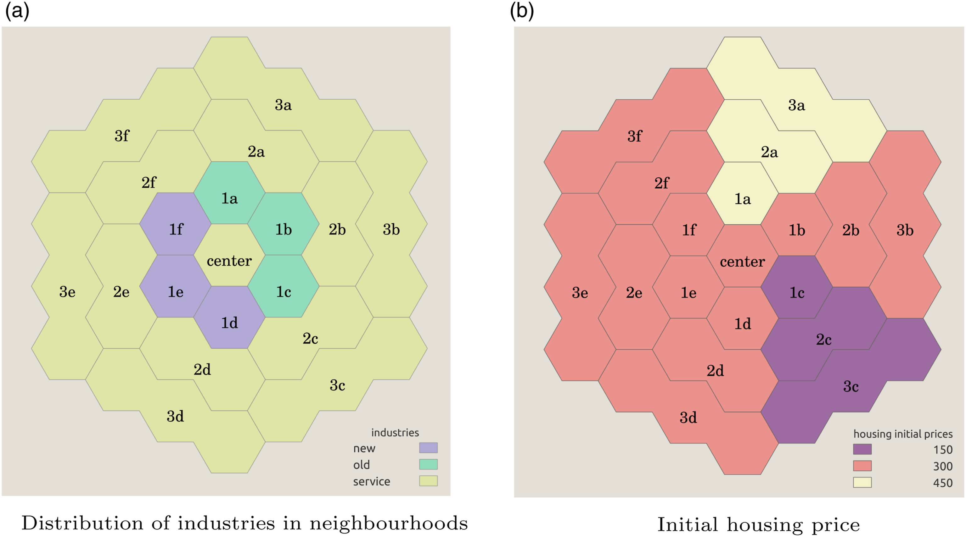
A business has workers and a target growth rate for the next period. A business will recruit new workers (from the local or global labour market) when expanding, or make existing ones redundant when downsizing. The target growth rate depends on the industries the businesses belong to. For those in the old and new industries, the target growth rate is exogenous and linked to the global scenario. For those in the service industry, it depends on the local market size. More details of the labour market can be found in Section 3.4.1. Figure 1 summarises the decision making process by different types of agents.

Figure 1.

Illustration of the coupled labour and housing markets.

Figure 2.

Spatial configuration of neighbourhoods at initialisation. Outer ring neighbourhoods are larger in size. Old industries concentrate in the northwest ring, just outside the city centre, whereas new industry locates in the southeast ring. Service businesses are scattered in all neighbourhoods and are more dense in the city centre. Initially, houses in southwestern areas (letter c) are cheaper, whereas houses at northwestern area (letter a) are more expensive.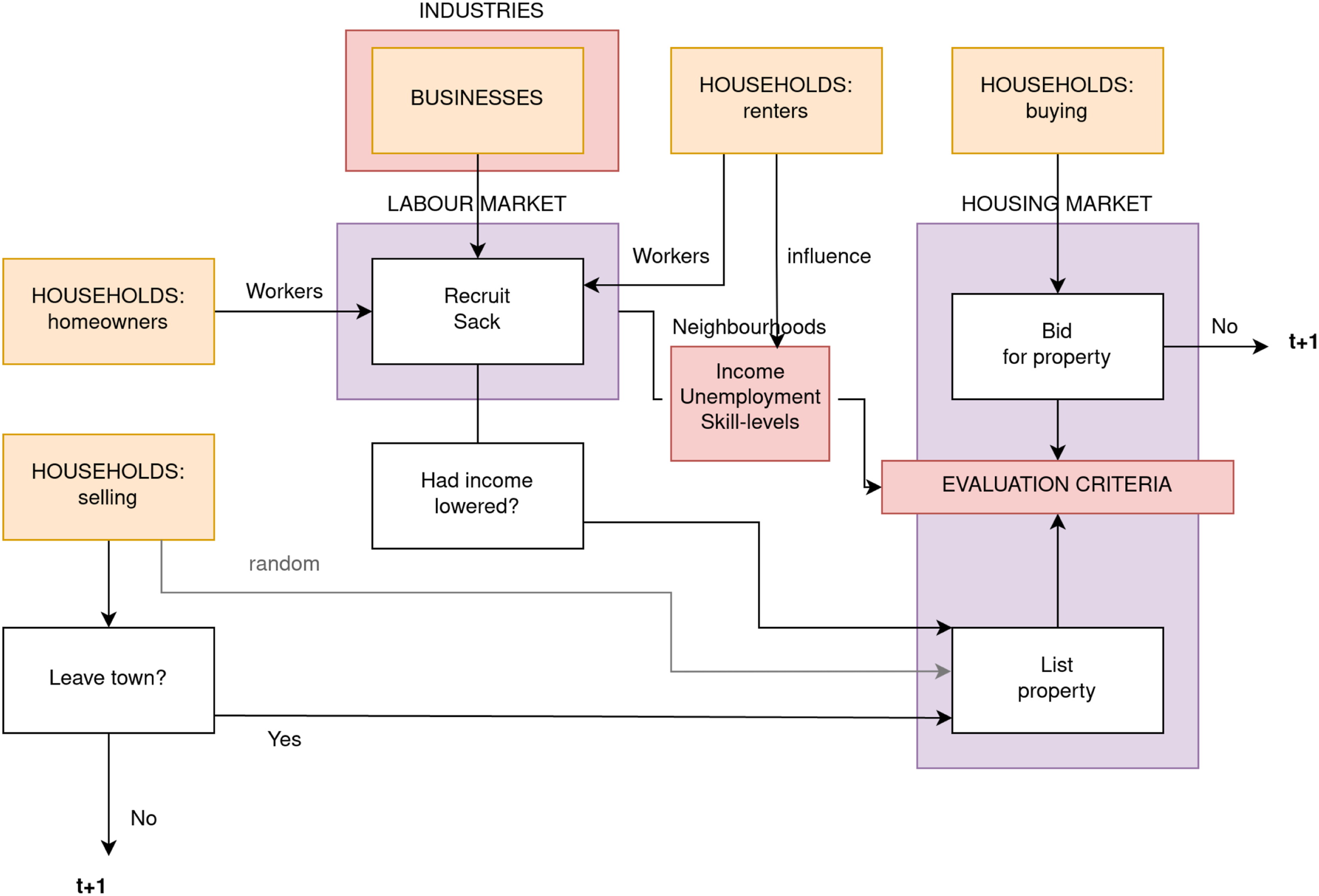

Spatial environment

The social and physical environment of the model include (1) three industries, to which the businesses belong to and (2) 19 neighbourhoods, in which houses and business are located (Figure 2). The three industries are old, new and service . The old and new are linked to the global market and have exogenous growth rates; whereas the service industry depends on the local market and thus has an endogenous growth rate. The industrial transition considered in this study is the collapse of the old industry and the transition to the new industry, with potential rippled effects on the service industry.

The model features a typical monocentric city that consists of 19 neighbourhoods as shown in Figure S1(a). The neighbourhoods are heterogeneous. The old and new industries are located only in certain neighbourhoods (2a). In the initialisation, all neighbourhoods have an equal number of service businesses, except for the city centre, which has twice as many service businesses (Figure S1(b)). Also, in the initialisation, some neighbourhoods have more expensive properties than others 2b. We introduce the initial differences in the neighbourhood to analyse the impact of urban transition on different neighbourhoods. We then assign households only to the neighbourhoods that their income can afford, which naturally result in differences in average household income and unemployment rate across neighbourhoods in the initialisation.

Micro-processes in urban transition

The temporal resolution in the model is weekly and the model is run for 10 years (or 520 weekly steps) after the initial burnout period (200 steps). We aim to study the medium-run dynamics, which is about 10 years. Rather than the short-run (just after the shock) or the long-run (when an equilibrium is reached), we believe that the medium-run is the most appropriate time frame to study the dynamic transition process of a city.

Labour market

The labour market features a searching and matching mechanism between job seekers (person agents) and hiring businesses (business agents). At the beginning of each period, businesses compare the target number of workers with the current number. If the target exceeds the current number, it will try to recruit workers from the local labour market first by posting a job advert detailing the minimum skill level required and income offered, which depend on the industry the business is in. We assume that the old and new industries have higher skill requirement and higher income on average compared with the service industry, although income of individual jobs will vary. Job adverts are open information to all. If multiple attempts to recruit from the local labour market have failed (e.g. no one applies or the one offered the job rejects), businesses will then recruit someone from the global labour market and bring new workers into the city. If, on the other hand, there are multiple applications for one job, the firm will hire the one with the highest skill level (more about skills in 3.4.4).

Unemployed workers will first seek jobs in the local labour market by browsing job adverts and making job applications to the hiring businesses. They will only apply for jobs for which their skill level exceeds the minimum requirement. We assume that job seekers do not have the time and cognitive capacity to browse all job adverts, so in each week, a job seeker will search a (random) subset of all the job adverts and apply for a maximum of three jobs with the highest income offered that they are eligible for.

If, however, unemployed skilled workers repeatedly fail to find a job, there is a probability that they will leave the city for job opportunities elsewhere. This is further complicated by their skill level and other members in the household. First, we assume that only skilled workers may find jobs elsewhere whereas unskilled workers cannot (or the wage level offered for unskilled worker do not support the move). This is a simplification, but is supported by literature which find that skilled workers are more mobile and adaptable and have a higher likelihood of finding jobs in different parts of the country (Autor, 2014; Yankow, 2006). Skilled workers leaving the city is one mechanism that causes the vicious cycle of brain drain, which the model aims to capture in the labour market dynamics (another is skill depreciation during long-term unemployment documented in 3.4.4). In addition, we assume that if there is another household member with a skilled job in the city, the family will not leave. Only when (1) the person is single or (2) the other household member is also unemployed or (3) the other household member works in an unskilled (service) industry, will a skilled person consider leaving for jobs elsewhere. In addition, the family owns a house in the city, they will also need to sell it first before moving out. The additional constraints are to acknowledge the complicated considerations of a household when making a relocation decision, which adds realism to the model.

Housing market

The housing market features a market settling process between sellers and buyers, both are household agents. In each period, homeowners will decide whether to sell their houses for various reasons, such as leaving the city or not being able to afford mortgage anymore. Those who decided to sell then list their house for sale on the housing market. Information on all houses for sale is open to all potential buyers, including information on the house (e.g. location, number of bedrooms, size etc.), asking price and time on market (TOM). A seller’s asking price depends on (1) past prices of similar properties in the neighbourhood (accounted for house price inflation) as reference price, and (2) the particular property’s TOM. The longer the house’s TOM, the more discount in asking price, as in Ge (2017).

Houses for sale are open information to all buyers. Since the houses are assumed to be uniform, households’ choice will depend on the asking price and the quality of the neighbourhood where the house is located. House evaluation will be based on the following elements: asking price, distance to work (average if there are more than one members in the household who are working), mean neighbourhood income (as a proxy for neighbourhood quality and amenity) and the percentage of skilled versus working class households (as a proxy for social class). Households will only consider houses for which the asking price is within their maximum budget, assumed to be 10 years of household income, a generous threshold set to allow for more flexibility (for comparison, in the UK lenders will typically lend up to 4.5–6 times one’s annual income).

After evaluating the houses for sale, the buyer will put in a bid on the house with the highest evaluation score if it exceeds their own minimum score. The bid price will similarly depend on the buyer’s TOM. The longer the buyer’s TOM, the higher the bid price w.r.t reference price. If a house gets multiple bids, the highest bid will be accepted. The final transaction price is the winning bid. In return, the relocation of households will change the endogenous features of the neighbourhood that they move into, including neighbourhood quality and social class (skilled vs working class).

The coupling of labour and housing market

The labour and the housing markets are coupled via the individual agents who are both employees (player in the former) and a household member (player in the latter). The spatial distribution of different industries will influence the local population and demand for housing in the nearby neighbourhoods. The income employees earned from the labour market will determine the household budget in the housing market. The employment status of household members will determine the household’s decision to buy, hold or sell a house, thus the supply and demand in the housing market. On the other hand, changes in the labour market and the neighbourhood composition will affect the demand for service workers there. We assume that people have the same access to jobs regardless of where they live, although in reality it is likely that people have better access to jobs near where they live, especially for low-income inner-city workers or those without a vehicle (Cervero et al., 1999). If we include that in the future, we may find that the housing market will have a bigger influence on the labour market. For example, we may observe a crowding-out effect that high housing price prevents people from accessing jobs there, which is found in expensive cities such as London (Turrell et al., 2018), New York and the San Francisco Bay area (Hsieh and Moretti, 2019).

Skill development and depreciation

Skills are single numeric values between 0 and 1 (1 = maximum) and is an attribute of a person agent. This is a simplification as skills and experience are specific to industries and occupations. In other words, we assume that skills developed in the old industry can be transferred fully to the new industry. Although in reality, there may be skill losses and re-training needed to transfer skills between industries, which could be added in future adaptations. We assume there are two types of industries: high-skilled and low-skilled ones. Both the old and new industries are high-skilled industries, and the service industry is considered low-skilled. To qualify to work in the high-skilled industry, one needs a minimum skilled level (assumed to be 0.5), whereas no minimum skill is required to work in the service industry.

All workers are endowed with a skill level at initialisation. The skill distribution in the population is in accordance with the industrial structure in the city (i.e. the percentage of high-skilled and low-skilled industries). While in employment, a worker’s skill level maintained the same. Moreover, one can also gain skills by participating in education or training if given the opportunity. On the other hand, if they are not in employment or training, one’s skill level depreciates. For every period, a person is not in employment or training, their skills will decrease by a small percentage, until it reaches the minimum. The loss of skill as a consequence of long-term unemployment is widely documented in the literature Schmieder et al. (2016); Görlich and De Grip (2008). For example, Edin and Gustavsson (2008) find that a full-year out of employment is associated with about 5% in skill loss. Skill depreciation is one cause of the brain drain self-reinforcing cycle that the model aims to capture (another being educated workers leaving the city (see more details in the ODD, Supplemental Material S1).

Spatial locked-in in rundown neighbourhoods

Previously, we discussed the effect of spatial locked-in (or housing locked-in) in declining cities: the sharp decline in housing value prevents house owners from moving out of declining neighbourhoods and regions to more prosperous ones. The model captures this effect by assuming that households have to sell their house first before moving out of the city. If household could not sell their house (e.g. because there are too many sellers and too few buyers), they will not be able to leave for better job opportunities elsewhere. The rationale is that households cannot afford the loss in resale value or need capital from resale to start a new life elsewhere. Ferreira et al. (2010) find that homeowners in the U.S. with negative equity (i.e. whose outstanding mortgage is more than the value of the house) are one-third less likely to move elsewhere, and every added $1000 in real annual mortgage costs lowers mobility by about 12%.

In a declining city, it is not uncommon to see housing values in rundown neighbourhoods plunge to nearly zero in some cases and homeowners there effectively locked into their current house and neighbourhood. Research also find that the decline in housing values is very unequal across neighbourhoods, with the best neighbourhoods suffer the least decline and the poorest ones suffer the most, exacerbating inequality within the city (Guerrieri et al., 2012). The effect of locked-in is further compounded by the deterioration of human capital with time (see 3.4.4): the longer the households have to wait to sell their house before they move out, the more their skills depreciates staying unemployed, and the harder they will find a job, creating a vicious cycle.

Agglomeration economies and the endogenous growth of the service industry

The model captures agglomeration economies in its simplest form: the endogenous growth of the service industry as a result of the growth or decline of local neighbourhoods. The growth rate for the old and new industries are exogenous and determined by external factors such as a paradigm shift in technology and global supply chain. The growth of the service industry, on the other hand, is endogenous and responds to changes in population and income in the local neighbourhood. The more prosperous the neighbourhood is, measured by the income level and the population who lives and works in the neighbourhood, the quicker the local service businesses (e.g. bakery, restaurants, supermarkets) grow and the more job opportunities they offer, and vice versa. Moreover, the more service businesses available in the neighbourhood, the more appealing the neighbourhood is to house buyers, which will attract more people to move there and further promote the growth of the service industry.

Of the three mechanisms of agglomeration economies, that is, sharing, matching and learning, the current version of the model captures only the first one, the sharing of markets and inputs. Hence it may underestimate the effect of agglomeration economies in urban transition. The other two mechanisms of matching and learning could be captured in future adaptations of the model, for example, by introducing industry-specific skills and the generation of new ideas as a result of spillover and crossover of knowledge enabled by skilled workers connecting with each other (via space or social network). This, however, is beyond the scope of this study and we believe it will over-complicate the model and should be left for future research.

Sensitivity analysis and calibration

We performed sensitivity analysis on the parameters of the model to make sure no single parameter changed the robustness of the results. Specifically, we checked that initial parameters related to skill, price and distance to jobs maintained reasonable, yet, varying results.

The sensitivity analysis involved testing 37 parameters within a range of three values for 10 simulation runs. For each parameter, 33 different indicators were plotted, displaying the mean and the top and bottom 5 quantiles. The purpose of the analysis was to identify which parameters had a significant impact on specific aspects of the model. We examined the primary indicators for all the parameters, followed by individual assessments of the housing and labour markets. Our aim was to ensure that altering a parameter’s value from its default, for example, from 0.01 to 0.005 or 0.02, would not cause a completely different trajectory in evaluating GDP, Gini coefficient, or unemployment.

Overall, the parameters were very robust, responding to value alterations without any disruptive behaviour. For instance, doubling the value of the parameter ‘Ask decrease per week’, which reduced the asking price for listed houses much faster, resulted in increased inequality among homeowners and non-homeowners. Other more significant changes produced expected results. Drastically reducing the order of magnitude of the Bid Discount parameter, for example, resulted in a marked increase in the time it takes to sell a house. Furthermore, amplifying the job search parameter from 1 to 3 produced minimal changes. Still, when the value was increased to 10, it resulted in a much better economic adjustment between workers and firms, leading to increased GDP, reduced inequality, higher income and lower unemployment.

In summary, we calibrated the parameters to provide a stable baseline that would enable clear comparisons with alternative scenarios. The results demonstrate that the model can handle value alterations without producing unexpected outcomes, making it a reliable tool for simulating the housing and labour markets.

Scenarios design

We have designed a number of alternative scenarios of exogenous shocks that enable the analysis of the model’s reaction to each one of them relative to a Baseline, business-as-usual path. All scenarios encompass a declining growth rate for the ‘old’, traditional industry, associated with varying degrees of expansion for a ‘new’, innovative industry.

The range of different scenarios together delineate distinct transitions and trajectory paths. These paths shed light on changes at the local level, specifically in neighbourhoods, across industries and in each specific market: housing and labour. Furthermore, they help us achieve the general goal of the model, which is to learn about the mechanisms that drive the divergent development of cities.

The unfolding of the scenarios cover a range of typical responses observed after a major shock, including collapse and decline, as seen in some of the cities mentioned in the introduction. Additionally, they explore possibilities of recovery, adaptation and transformation, as discussed in (Eraydin and Özatağan, 2021). Implementing these scenarios is relatively straightforward and involves changing the external growth rate of the industries and adjusting the magnitude of the training parameter, specifically for the Enhanced Training (Training) scenario (from 0.01 to 0.1, see Table 1).

Table 1.

Monthly growth rates (GR) for old and new industries throughout different scenarios.

Scenarios	GR–Old	GR–New	Observations
Baseline	0.00	0.00	Status quo
Total collapse	−0.01	0.0005	—
Transition	−0.002	0.002	—
Enhanced training (Training)	−0.002	0.002	Increased training probability
Global recruit	−0.01	0.005, 0.001*	Increased global recruit of workers
Weak recovery	−0.002	0.0005	—

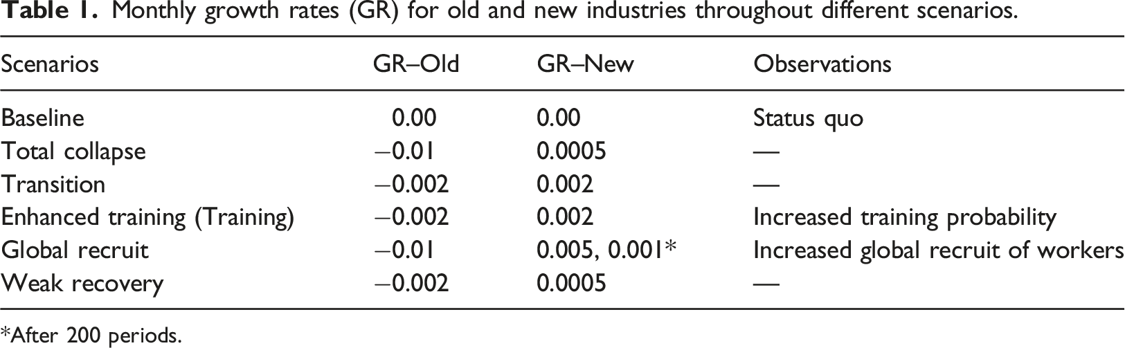
*After 200 periods.

The Baseline scenario serves as a status quo in which all industries remain unchanged. Total Collapse features a sudden, drastic collapse of the main industry in the city followed by long-term stagnation, as are often observed in many former industrial cities such as Detroit, Leipzig and Liverpool (Rink et al., 2012). On the contrary, Global Recruit features a quick and aggressive expansion of the new industry, which could cause a social, economic or infrastructural ‘overshoot’ beyond a city’s capacity. This overshooting can lead to complex problems such as increased inequality, high cost of living, disruption of communities and heightened social tension, and could pose a significant risk for cities undergoing major industrial shifts. Gyourko et al. (2013) discusses how economic growth fuelled in part by a large influx of high-skilled workers in the ‘superstar cities’ like San Francisco has crowded out lower income households and contributed to increased inequality. Another example for infrastructural overshoot is China’s numerous ghost towns and neighbourhoods as a result of aggressive state-led housing and urban development programmes (Shepard, 2015).

Transition and Training both feature a more gradual and smooth transition to the new industry. The difference is that the latter provides re-training opportunities to the workers to enhance their skill levels, which mitigates skill depreciation that occurs during unemployment and allows more workers to be eligible for jobs in the (high-skilled) new industry. Finally, Weak Recovery features a slow decline in the old industry and slow growth in the new industry.

The growth rates are chosen so that at the end of the simulation, the old industry will almost disappear in Total Collapse and Global Recruit, and the new industry will more than replace the old in the growth scenarios. They are also chosen to reflect the relative magnitude of industrial decline and growth across scenarios.

Results

We present four distinct groups of results: at the macroeconomic and the neighbourhood level, and for the housing and labour markets. Due to space restrictions, we provide additional results at section 2 of the Supplementary Material 1.

Macroeconomic results

In all scenarios, the total GDP Figure S3(a) declines at the beginning of the shock as the old industry collapses. The dip in GDP is smallest under Transition and Training. Under Global Recruit, the GDP recovers most quickly before it surpasses the baseline. The recovery path is more volatile under Global Recruit. The GDP and population (Figure S3(b)) in both Weak Recovery and Total Collapse scenarios keep declining throughout the simulation.

Initially housing price index (3c) declines at the wake of the shock, as people who have lost jobs in the old industries try to sell their houses, with the deepest drop under Total Collapse and Global Recruit. Under some scenarios, including Transition, Training and Global Recruit, housing price recovers and rise to a level higher than that under baseline. Under Weak Recovery and Total Collapse, on the other hand, housing prices never return to the pre-shock level. Under Weak Recovery properties maintain more than half of its original values at the end of the simulation, whereas they lost almost all of their values under Total Collapse. Unemployment rate is defined as the percentage of people who are without a job in the total (working) population. As expected, unemployment rate is much higher under Total Collapse (∼40%) and Weak Recovery (∼25%) (3d). The relatively aggressive nature of growth under Global Recruit means that a large number of unemployed workers from the city’s old industry cannot find jobs in the new sectors, which becomes a long-term unemployment issue overtime. Unemployment rate is the lowest in Training, although still higher than Baseline at the end of the simulation.

At the beginning of the shock, income inequality increases, due the collapse and the lost income in the old industry (3e). Under Transition and Training, inequality starts to decline after a while. Under Training, it even drops below the Baseline in the last 100 periods, which shows that training can lead to a more equality income distribution by allowing more people to access high-income jobs. On the other hand, income Gini is much higher under Global Recruit, which features a scenario with higher growth in GDP but also higher inequality. Home equity is an important source of wealth for households. Changes in property values can therefore create inequality in wealth among homeowners and non-homeowners. In this model, wealth is measured by household’s net gains or losses from changes in housing price (i.e. current value net of purchase price). Figure 3(f) shows that wealth Gini is the highest under Total Collapse, followed by Global Recruit, which reflects the high volatility in housing prices.

Figure 3.

Macroeconomic results under different scenarios.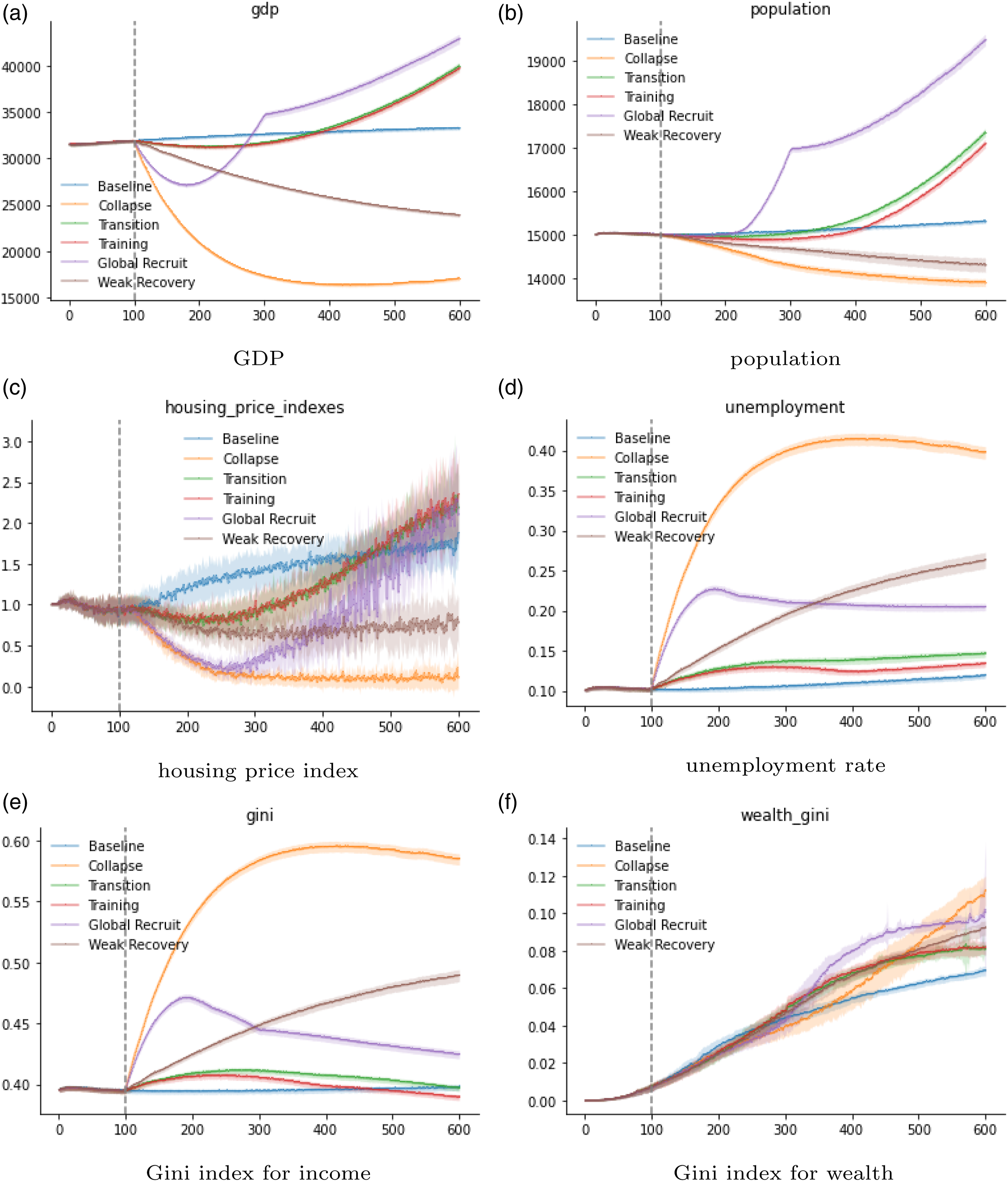

Housing market

During the initial shock, all scenarios see the number of houses for sale increase, as people who have lost their jobs in the old industry sell their houses (4a) (Figure 4). Under Total Collapse and Global Recruit, in particular, the number of houses for sale jump to 5–6 times the pre-shock level. The average time-on-market reflects the general housing market conditions (4b). Under Total Collapse and Global Recruit, the impact of the shock is significant. Under Total Collapse, especially, the TOM keeps rising to a staggering 150 periods (3 years in real time), meaning that houses are not selling while losing its value overtime. That means people may be stuck in a declining city.

Figure 4.

Housing market indicators under different scenarios.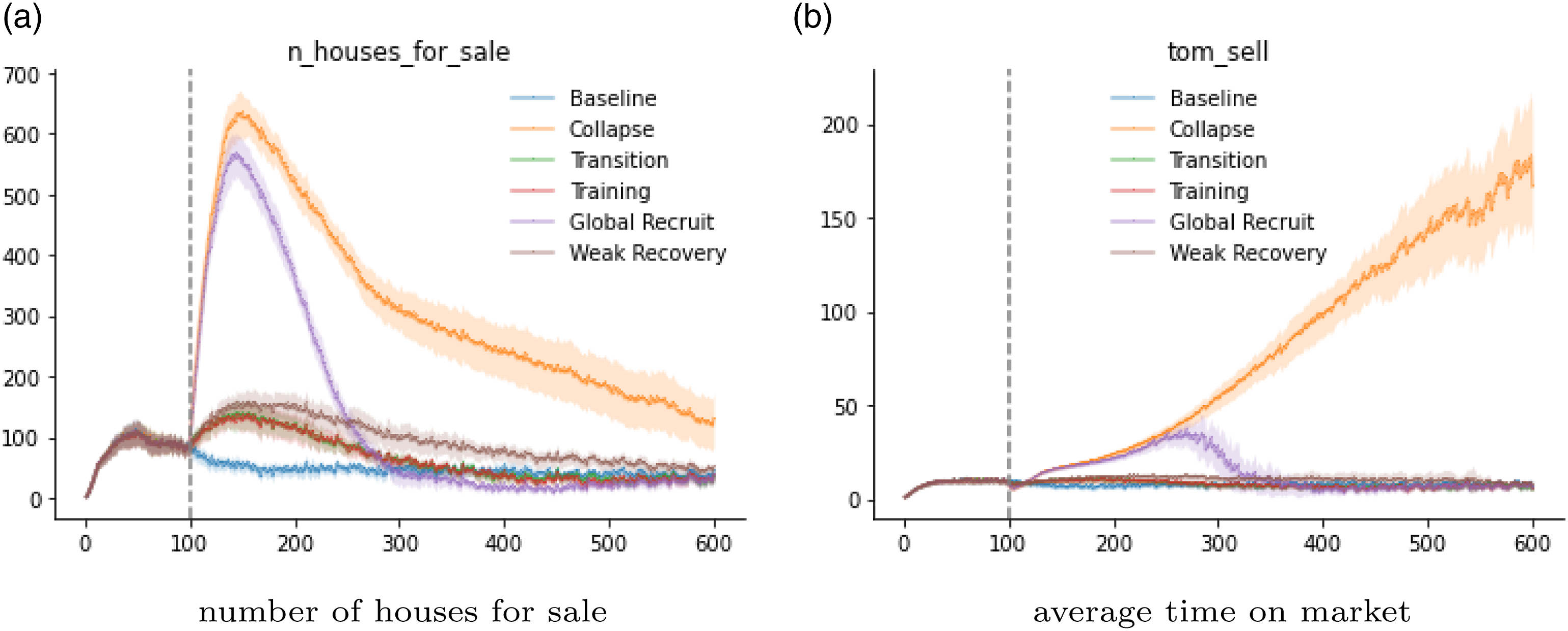

Labour market

As expected, there is an initial jump in both the number of job adverts and new recruits from outside the city under Global Recruit, which features an initial rapid expansion of the new industry and an aggressive recruitment strategy to introduce skilled workers from outside of the city (Figures 5(a) and (a)). Global Recruit scenario sees the largest increase in the number of jobs adverts in the new industry at the beginning of the transition (Figure 5(c)). However, under Total Collapse, the number of jobs available in the new industry does not increase, with a significantly increase in the number of applicants (Figure 5(d)). This indicates a severe imbalance in the labour market, where a large number of unemployed skilled workers (they can only apply if their skill level qualifies) are looking for jobs in the new industry, but available job opportunities are extremely limited.

Figure 5.

Labour market results under different scenarios.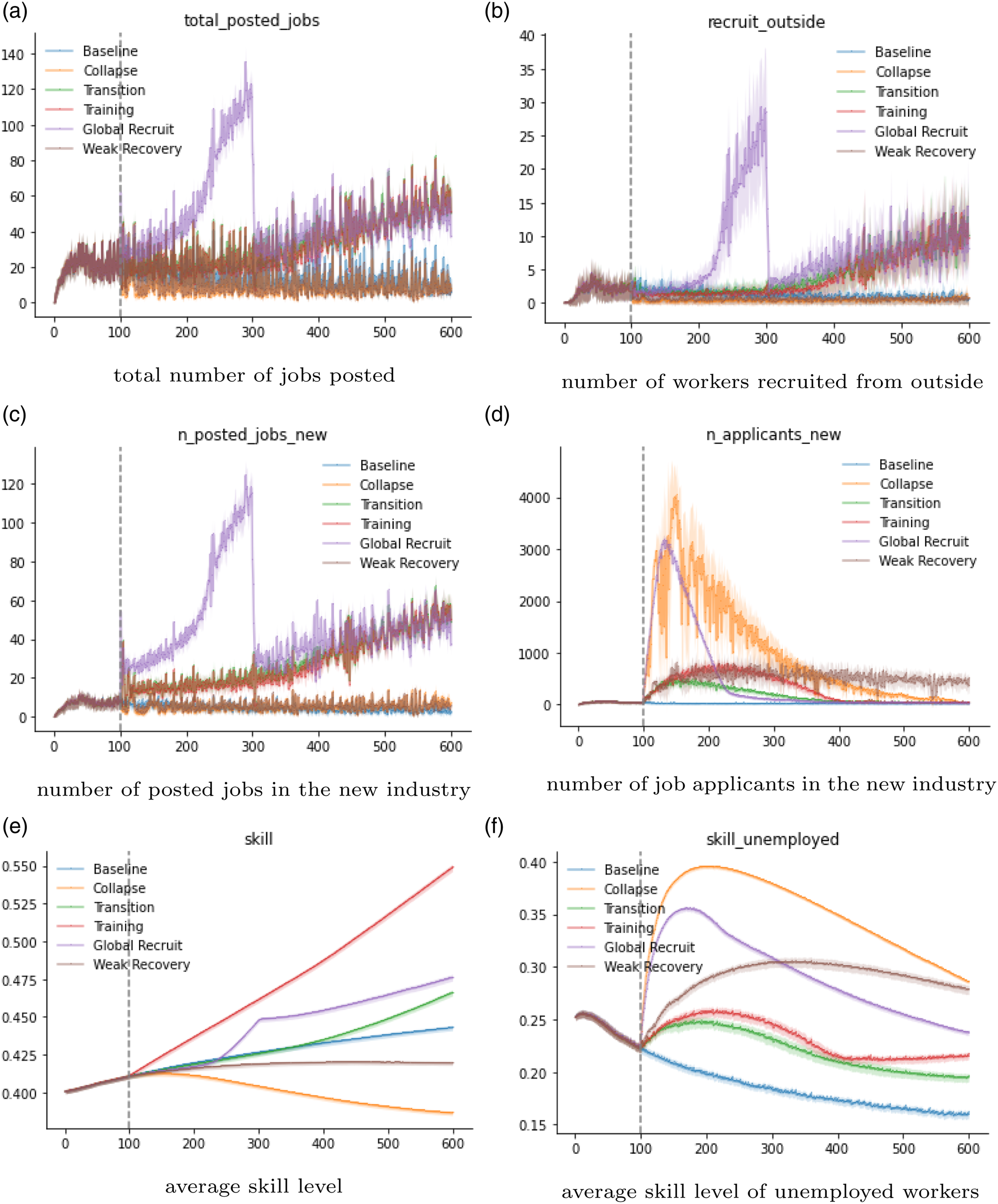

The average skill level is the highest under Training, as a result of the extra training opportunities provided to the whole population (Figure 5(e)), seconded by Global Recruit, because of the influx of skilled workers attracted by the rapidly expanding new industry. A decline in the average skill level in the population reflects the depreciation of human capital in the city. The skill level of the unemployed people (Figure 5(f)) has two sides. On the one hand, it reflects the human capital reservoir available in the city. On the other hand, as the skills are not currently put to use, it shows the waste of human resources. Under Total Collapse and Weak Recovery, the average skill of unemployed workers is much higher than in the Baseline, indicating a waste of human resource as many skilled workers are unemployed. Finally, there is an increase in skills under Training due to more training opportunities offered to unemployed people.

Neighbourhood results

Under Baseline (6a), all neighbourhoods experience a moderate level of inflation in the housing prices, with the poorest neighbourhoods seen the largest inflation (around 100%). The city centre, on the other hand, sees the smallest inflation in housing price (around 20%). Under Total Collapse (6b), however, all neighbourhoods see a significant drop in housing prices. Yet the level of price drop is unequal across neighbourhoods, which is consistent with existing findings (Jiang et al., 2021; Guerrieri et al., 2012).

Under the two transition scenarios (Figures 6(c) and (d)), price inflation in poor neighbourhoods are much higher than the rest. The overall level of inequality in housing price among neighbourhoods decreases as a result of transition. Housing price indexes are more turbulent under Global Recruit (Figure 6(e)). However, the level of volatility vary greatly across neighbourhoods, with the rich neighbourhoods seen the least volatility. Finally, under Weak Recovery, only the rich neighbourhoods manage to maintain its property values, and all the other neighbourhoods see its property value decrease. The differences in the growth rate will greatly exacerbate the level of inequality in property values across neighbourhoods.

Figure 6.

House price index in different neighbourhoods.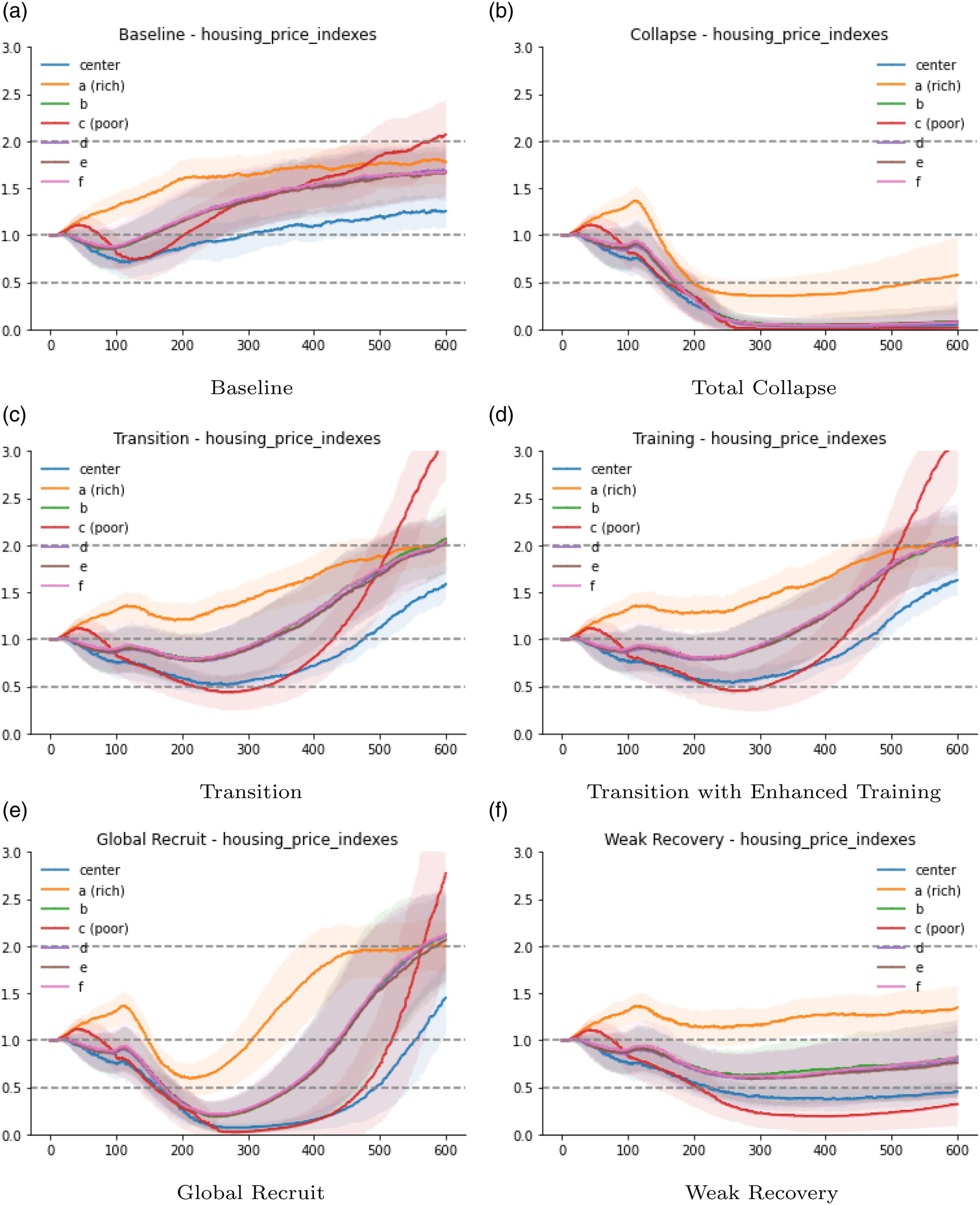

Discussion

The different growth scenarios have a profound impact on the path of the city and its heterogeneous neighbourhoods. As expected, in Total Collapse where the old industry has collapsed but the new industry barely grows, the results are devastating, which include lasting high unemployment rate and the collapse of the housing price in almost all neighbourhoods. Interestingly, the model also shows potential side effects from Global Recruit where the new industry grows rapidly fuelled by the recruit of skilled workers globally, including higher overall unemployment rate and inequality, a phenomenon observed in many countries and cities during the recent globalisation (Bourguignon, 2013).

Additionally, Global Recruit has led to higher GDP and growth rate, as well as higher average skill level or human capital in the city. The influx of skilled workers into the city do not only benefit the new industry but also the locals by increasing the number of jobs in the service industry and driving up the local wage level. It also increases the demand for housing and drives up housing prices in certain neighbourhoods.

However, not everyone will benefit from the growth. Results show that unemployment rate remains significantly higher than the Baseline years after the collapse of the old industry, indicating that growth in the new industry cannot fully absorb the local workforce, especially as workers gradually lose their skills over the years of unemployment (Laureys, 2021). Moreover, jobs taken by the locals in the service industry pays a lot less than those in the new industry where most foreign workers cluster, meaning that the income gap between the locals and the newcomers have widened. In terms of local human capital, although Global Recruit increases the local human capital by introducing a large number of global skilled workers into the city, other growth path such as Training can achieve the same or even higher level in the long-run by providing training to the local residents.

Compared with a more gradual growth strategy such as Transition or Training, Global Recruit has also led to more volatility in the housing market, which in turn leads to higher inequality in wealth (in the form of home equity). Using a one-to-one scale ABM of roughly 25 million UK households, Guerrero (2020) investigated the role of market institution and housing price on wealth inequality, and estimated that the decentralised housing market contributes to about one to two thirds of the Gini coefficient in the UK. Especially during an urban transition when the labour and the housing market are experiencing increased volatility as well as long-term shifts, the effect of the housing market and price on wealth inequality can be magnified.

Furthermore, we find that poor neighbourhoods benefits the most from the growth of the new industry. The gaps in housing price between the rich and poor neighbourhoods closes under scenarios with steady or rapid growth in the new industry and widens under those with slow or no growth. In the latter, only the rich neighbourhoods maintain most of its property values, whereas poor neighbourhoods lost most of its property values, which is consistent with empirical evidence. Lastly, the city centre, where there are more service businesses, has lagged behind others in the growth of income and housing price in most scenarios, mainly because the service industry has a lower income level and growth rate compared with the new industry.

The model has important policy implications. It suggests several recommendations that align with empirical findings. Firstly, policymakers should prioritise immigration that brings in new skilled workers as a way to stimulate industry replacement and alternative expansions. Secondly, fast industry decay disproportionately affects residents and the value of poorer neighbourhoods, which calls for specific, place-based planning and development to alleviate these effects. Thirdly, during periods of slow industry growth, new industries tend to grow more unequally across city space. Policymakers should therefore pay attention to inequality and consider policies that provide redistribution and social welfare. Lastly, training programmes that maintain and upgrade workers’ skills towards a possible replacing industry are essential in the face of significant industry decay.

There are many simplifications in the model. For example, there are no investors in the housing market, which may be added to study their role on the housing price or the forming of a housing bubble. The growth rate in the new industry is assumed to be exogenous and the skills of workers fully transferable from the old industry to the new one. The complex process of innovation and the mechanism behind the growth of an industry is beyond the scope of the study. In the future, the model can be coupled with a production model with endogenous innovation and growth to study the dynamics between innovation, human capital, productivity growth and urban transition.

U-TRANS is purposefully developed at an abstract level with the flexibility to be tailored for a specific city. The three-ring urban layout and the stylised industrial structure (old, new and service) are chosen to create a simple but useful structure for the designed scenarios and experiments. The model is a first step towards a dynamic modelling framework of urban transition under the influence of a socio-economic and technological shock.

Concluding remarks

U-TRANS provides a relatively simple but useful modelling framework to study urban transition from the bottom up. By coupling the endogenous labour and housing markets, we can use it to explore different transition scenarios and strategies. The model incorporates some key interacting factors and micro processes, including individual workers and households, human capital, industrial structure, businesses and neighbourhoods. By simulating different transition scenarios, U-TRANS is able to generate similar patterns as observed in urban transitions in the real world, including the different housing market dynamics in rich and poor neighbourhoods, the division between local and international workers, and the trade-off between growth and inequality in both income and wealth. In the future, the framework can be adapted to a specific city using city-specific data, or be coupled with models of innovation to study the impacts of innovation and industrial revolution on the development paths of cities.

Supplemental Material

Supplemental Material - Modelling urban transition with coupled housing and labour markets

Supplemental Material for Modelling urban transition with coupled housing and labour markets by Jiaqi Ge and Bernardo Alves Furtado

Footnotes

Declaration of conflicting interests

The author(s) declared no potential conflicts of interest with respect to the research, authorship, and/or publication of this article.

Funding

The author(s) received no financial support for the research, authorship, and/or publication of this article.

ORCID iDs

Jiaqi Ge

Bernardo Alves Furtado

Supplemental Material

Supplemental material for this article is available online.

Jiaqi Ge a University Academic Fellow (UAF) in the School of Geography at the University of Leeds. Her research areas are agent-based modelling, behavoural modelling in complex systems, urban transition and housing markets. Her research develops agent-based models to study urban transition under major socio-economic and environmental shocks, such as climate change and the fourth industrial revolution. Her research contributes to the understanding of how cities as self-organised complex systems adapt to external shocks and evolve under a changing environment. Jiaqi is originally from Shanghai, China.

Bernardo Alves Furtado is a senior researcher at the Institute for Applied Economic Research, a government-affiliated think-tank in Brazil. His expertise lies in spatial analyses, urban economics, real estate, municipalities and metropolitan regions. With a PhD from Utrecht University in co-tutorship with a PhD in Economics from UFMG, Bernardo's research currently focuses on applying agent-based modelling techniques to analyse and inform public policy.

References

Alves Furtado

(2022) Policy space 2: modeling markets and endogenous public policies. Journal of Artificial Societies and Social Simulation 25(1): 8.

Austin

Glaeser

Summers

(2018) Jobs for the Heartland: Place-Based Policies in 21st Century America. Brookings Papers on Economic Activity, vol 2018(1), pages 151-255.

Autor

(2014) Skills, education, and the rise of earnings inequality among the “other 99 percent”. Science 344(6186): 843–851.

Axtell

Guerrero

López

(2019) Frictional unemployment on labor flow networks. Journal of Economic Behavior and Organization 160: 184–201.

Benner

(2003) Learning communities in a learning region: the soft infrastructure of cross-firm learning networks in silicon valley. Environment and Planning A: Economy and Space 35(10): 1809–1830.

Bettencourt

LMA

West

(2010) A unified theory of urban living. Nature 467(7318): 912–913. http://www.nature.com/nature/journal/v467/n7318/full/467912a.html

Bonabeau

(2002) Agent-based modeling: methods and techniques for simulating human systems. Proceedings of the National Academy of Sciences of the United States of America 99(suppl_3): 7280–7287.

Bourguignon

(2013) The globalisation of inequality. EUI MWP LS 49, p. 56Z. https://cadmus.eui.eu/handle/1814/26496 Accepted: 2013-04-04T15.

Campante

Glaeser

(2018) Yet another tale of two cities: Buenos aires and Chicago. Latin American Economic Review 27(1): 2–33.

10.

Cervero

Rood

Appleyard

(1999) Tracking accessibility: employment and housing opportunities in the san francisco bay area. Environment and Planning A: Economy and Space 31(7): 1259–1278.

11.

Chan

(2001) Spatial lock-in: Do falling house prices constrain residential mobility? Journal of Urban Economics 49(3): 567–586. https://www.sciencedirect.com/science/article/pii/S0094119000922058

12.

Dawid

Gemkow

Harting

, et al. (2014) Agent-based macroeconomic modeling and policy analysis: the eurace@ unibi model. Bielefeld Working Papers 01: 1–27.

13.

Dosi

Fagiolo

Roventini

(2006) An evolutionary model of endogenous business cycles. Computational Economics 27(1): 3–34.

14.

Edin

P-A

Gustavsson

(2008) Time out of work and skill depreciation. ILR Review 61(2): 163–180.

15.

Eraydin

Özatağan

(2021) Pathways to a resilient future: a review of policy agendas and governance practices in shrinking cities. Cities 115: 103226. Publisher: Elsevier.

16.

Ettema

(2011) A multi-agent model of urban processes: modelling relocation processes and price setting in housing markets. Computers, Environment and Urban Systems 35(1): 1–11.

17.

Ferreira

Gyourko

Tracy

(2010) Housing busts and household mobility. Journal of Urban Economics 68(1): 34–45.

18.

Filatova

(2015) Empirical agent-based land market: integrating adaptive economic behavior in urban land-use models. Computers, Environment and Urban Systems 54: 397–413.

19.

(2017) Endogenous rise and collapse of housing price: an agent-based model of the housing market. Computers, Environment and Urban Systems 62: 182–198.

20.

Polhill

Craig

, et al. (2018) From oil wealth to green growth-an empirical agent-based model of recession, migration and sustainable urban transition. Environmental Modelling and Software 107: 119–140.

21.

Geanakoplos

Axtell

Farmer

, et al. (2012) Getting at systemic risk via an agent-based model of the housing market. American Economic Review 102(3): 53–58.

22.

Gilbert

Hawksworth

Swinney

(2009) An agent-based model of the english housing market. AAAI Spring Symposium: Technosocial Predictive Analytics. Palo Alto, California USA: AAAI Press, 30–35.

23.

Glaeser

(2010) Agglomeration Economics. University of Chicago Press.

24.

Glaeser

Ponzetto

, et al. (2010) Did the death of distance hurt detroit and help new york? Agglomeration Economics 303: 303–305.

25.

Görlich

De Grip

(2008) Human capital depreciation during hometime. Oxford Economic Papers 61(suppl_1): i98–i121.

26.

Goudet

Kant

J-D

Ballot

(2017) Work sim: a calibrated agent-based model of the labor market accounting for workers’ stocks and gross flows. Computational Economics 50(1): 21–68. https://doi.org/10.1007/s10614-016-9577-0

27.

Grimm

Railsback

Vincenot

, et al. (2020) The odd protocol for describing agent-based and other simulation models: a second update to improve clarity, replication, and structural realism. Journal of Artificial Societies and Social Simulation 23(2): 1–20.

28.

Guerrero

(2020) Decentralized markets and the emergence of housing wealth inequality. Computers, Environment and Urban Systems 84: 101541. https://www.sciencedirect.com/science/article/pii/S019897152030274X

29.

Guerrero

Axtell

(2013) Employment growth through labor flow networks. PloS One 8(5): e60808.

30.

Guerrieri

Hartley

Hurst

(2012) Within-city variation in urban decline: the case of detroit. American Economic Review 102(3): 120–126.

31.

Gyourko

Mayer

Sinai

(2013) Superstar cities. American Economic Journal: Economic Policy 5(4): 167–199.

32.

Haase

Lautenbach

Seppelt

(2010) Modeling and simulating residential mobility in a shrinking city using an agent-based approach. Environmental Modelling and Software 25(10): 1225–1240. https://www.sciencedirect.com/science/article/pii/S1364815210001027

33.

Hsieh

C-T

Moretti

(2019) Housing constraints and spatial misallocation. American Economic Journal: Macroeconomics 11(2): 1–39.

34.

Jacobs

(1985) Cities and the Wealth of Nations: Principles of Economic Life. New York: Vintage.

35.

Jiang

Crooks

Wang

, et al. (2021) Simulating urban shrinkage in detroit via agent-based modeling. Sustainability 13(4): 2283.

36.

Kemeny

Storper

(2012) The sources of urban development: wages, housing, and amenity gaps across american cities. Journal of Regional Science 52(1): 85–108.

37.

Kroft

Lange

Notowidigdo

(2013) Duration dependence and labor market conditions: evidence from a field experiment. The Quarterly Journal of Economics 128(3): 1123–1167.

38.

Krugman

(1996) The Self Organizing Economy. Massachusetts: Blackwell Publishers Ltd Malden.

39.

Laureys

(2021) The cost of human capital depreciation during unemployment. The Economic Journal 131(634): 827–850.

40.

López

Gaspard

Axtell

(2020) Predatory publishing and the academic librarian: developing tools to make decisions. Medical Reference Services Quarterly 39(1): 1–14.

41.

Magliocca

Safirova

McConnell

, et al. (2011) An economic agent-based model of coupled housing and land markets (chalms). Computers, Environment and Urban Systems 35(3): 183–191.

42.

Martin

(2016) Divergent urban economic development: reflections on a tale of two cities. Regional Studies 50(9): 1623–1627.

43.

Nichols

Mitchell

Lindner

(2013) Consequences of Long-Term Unemployment. Washington, DC: The Urban Institute. Technical report.

44.

Ortego-Marti

(2017) Differences in skill loss during unemployment across industries and occupations. Economics Letters 161: 31–33.

45.

Parker

Filatova

(2008) A conceptual design for a bilateral agent-based land market with heterogeneous economic agents. Computers, Environment and Urban Systems 32(6): 454–463.

46.

Puga

(2010) The magnitude and causes of agglomeration economies. Journal of Regional Science 50(1): 203–219.

47.

Rink

Haase

Grossmann

, et al. (2012) From long-term shrinkage to re-growth? the urban development trajectories of liverpool and leipzig. Built Environment 38(2): 162–178.

48.

Schmieder

von Wachter

Bender

(2016) The effect of unemployment benefits and nonemployment durations on wages. American Economic Review 106(3): 739–777.

49.

Shepard

(2015) Ghost Cities of China: The Story of Cities without People in the World’s Most Populated Country. London, UK: Bloomsbury Publishing.

50.

Simmie

Martin

(2010) The economic resilience of regions: towards an evolutionary approach. Cambridge Journal of Regions, Economy and Society 3(1): 27–43.

51.

Storper

Kemeny

Makarem

, et al. (2015) The Rise and Fall of Urban Economies: Lessons from San Francisco and Los Angeles. Stanford, CA: Stanford University Press.

52.

Swanstrom

Dreier

Mollenkopf

(2002) Economic inequality and public policy: The power of place. City and Community 1(4): 349–372.

53.

Tong

Guerrero

Lopez

, et al. (2017) Diffusing workers in a multiplex world. Saïd Business School WP 21: 8.

54.

Turrell

Speigner

Djumalieva

, et al. (2018) Using Job Vacancies to Understand the Effects of Labour Market Mismatch on uk Output and Productivity. Bank of England Working Paper. Technical report.

55.

Yankow

(2006) Why do cities pay more? an empirical examination of some competing theories of the urban wage premium. Journal of Urban Economics 60(2): 139–161.

Supplementary Material

Please find the following supplemental material available below.

For Open Access articles published under a Creative Commons License, all supplemental material carries the same license as the article it is associated with.

For non-Open Access articles published, all supplemental material carries a non-exclusive license, and permission requests for re-use of supplemental material or any part of supplemental material shall be sent directly to the copyright owner as specified in the copyright notice associated with the article.

0.00 MB

1.46 MB