Sage Journals: Discover world-class research

Abstract

Bicycle networks are made up of different types of infrastructure for cars, bikes and mixed use, which has resulted in various definitions being used to describe them. However, it’s crucial to bring these definitions together to understand the structural differences among them and the impact of choices and investments in bike infrastructure. This study examines different definitions of bicycle networks in 47 cities, analysing scaling effects and various network metrics for four different definitions. Understanding structural characteristics of different bicycle networks definitions contributes to the body of knowledge necessary for design interventions by policymakers.

Keywords

Bicycle networks scaling relations complex network analysis

Introduction

Biking is looked upon as an efficient and sustainable means of transportation. It has a huge impact on reducing congestion, and various forms of pollution, and is a major driver in promoting active and healthy lifestyles. Yet, in practise, we often see that bicycle infrastructure is disadvantaged by providing a limited amount of space for it Szell (2018); Gössling et al. (2016), and a highly fragmented street network Orozco et al. (2020). Based on the spatial structure of a city and the activity patterns of its inhabitants, policymakers have to decide how limited and contested space is distributed between the different transport modes. It is challenging to allocate dedicated space to bicycle infrastructure, as traditionally street networks are designed for car-use and can often be substituted for informal biking.

Traditional street networks are made of different infrastructure types for car-use, bicycles or mixed use OSM (2021b). Street networks used for cars are efficient and well-connected: the amount of street infrastructure per capita decreases as population increases Bettencourt (2013). To promote other active forms of transportation (e.g. biking) policymakers require a fundamental understanding of how these infrastructure types scale with the size of a city population, and how can they be expanded or developed.

Multiple scholars have advanced our understanding of bicycle networks Mekuria et al. (2012); Schoner and Levinson (2014); Buehler and Dill (2016); Orozco et al. (2020). But some studies attempting to define bicycle networks have done so in an ad-hoc manner, which makes results difficult to replicate and generalise, and provide tailored evidence to policymakers for targeted interventions in the expansion and design of bicycle infrastructure. This ultimately impedes building upon previous findings and slows the epistemological advances in the domain of active mode infrastructure. Bicycle networks can be defined by considering the aggregation of different infrastructure types. Identifying which infrastructure types make-up a bicycle network is not easy, yet it highly impacts the results of space allocation studies by making a city seem more bike-friendly than it is if one considers a bike network made of all streets where it is possible (instead of safe or comfortable) to cycle on. As summarised in Figure 1, studies on space allocation and network characteristics have adopted very different bicycle networks definitions Murphy and Owen (2019); Wu et al. (2021); Szell (2018); Nello-Deakin (2019), which inevitably affect the result of the analysis and hinders any type of comparison between studies.

Figure 1.

Previous studies on space allocation and network analysis have used different definitions of bicycle networks.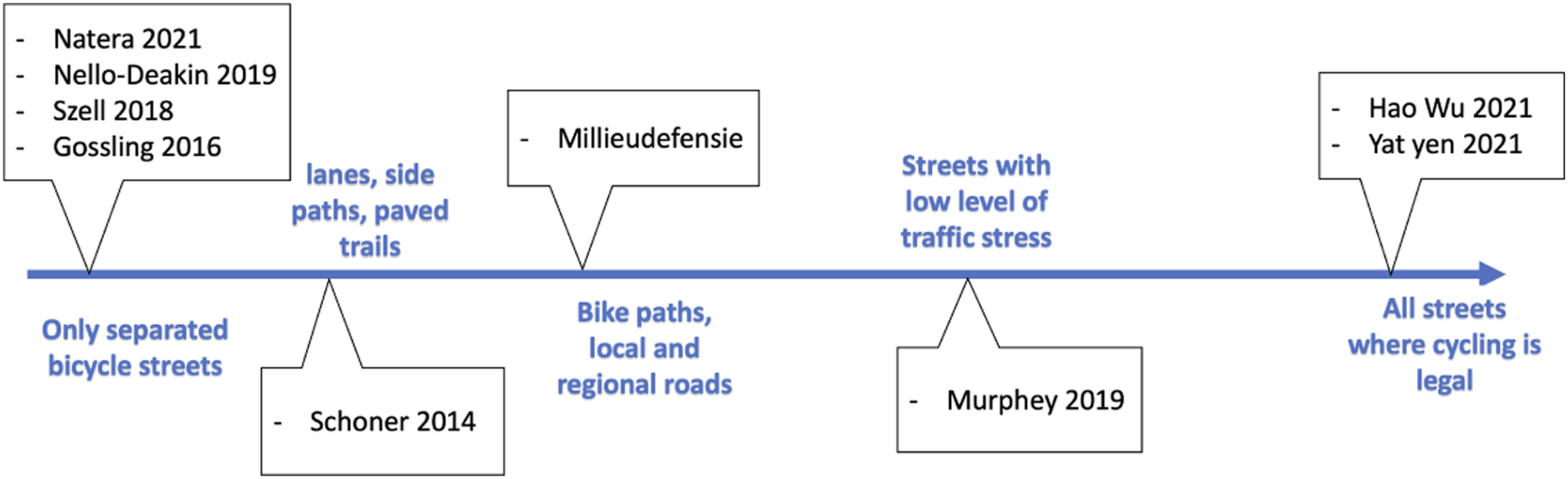

Moreover, previous research suggests that, adding bike infrastructure (dedicated or shared) may not be enough to stimulate bicycle use, if it does not reinforce the network structure (e.g. density and connectivity) Schoner and Levinson (2014). Thus, it is crucial to bring together the definitions of bicycle networks and compare structural differences among them to understand consequences of the choices and investments made in bike infrastructure networks. A comparison between bicycle network definitions would identify the positive or negative structural characteristics of different bicycle network definitions, which ultimately influence bicycle attractiveness Kamel and Sayed (2021). A multi-city comparison with common definitions of bicycle networks would bridge this gap by systematically analysing the same networks over multiple cities to identify worldwide relations, thus contributing to the body of knowledge necessary for design interventions by policymakers.

In this article, we systematically define and analyse different types of bicycle networks to understand how the city size affects infrastructure development per mode and if the selected bicycle network definition affect characteristics of the network. We apply the analysis to 47 cities to provide empirical evidence and facilitate comparison in structural properties of the networks. We structure the analysis by asking two questions:

1. As larger cities build less infrastructure per capita, how do the different infrastructure types scale with city size and how is the scaling relation of the different bicycle network definitions affected?

2. As different definitions of bicycle network exist, how can we provide evidence-based knowledge on the structural differences and similarities of bicycle networks worldwide?

Understanding the scaling relations between infrastructure types and city size can unravel how demographic changes in cities, resulting from increasing urbanisation, will impact the transport system and ultimately the travel behaviour of residents. We carry out a novel bicycle network analysis over multiple cities and multiple network definitions. Our findings will help researchers understand the different structural properties of bicycle network definitions and their impact on network evaluation methods. Policymakers will be able to identify the bike network that meets their policy objectives. This analysis is particularly relevant now given the ‘window of opportunity’ that the COVID-19 pandemic has created for many policymakers to convert car-dominated streets into bike lanes. Our analysis, for example, shows the changes in structural properties if a city makes all its residential streets truly bikeable. Moreover, our numerical analysis will provide unique benchmark values that urban planners can use to set their network objectives against the average or best-performing cities.

This manuscript is structured as follows. In the Methodology section we present the network data and methods used. Then the Empirical Analysis and Results section illustrates the outcome of the analysis for 47 cities. The Implications for practice section discusses practical relevance. Finally, the Discussion and Conclusions section follows.

Methodology

The goal of this study is to understand how the city size affects infrastructure availability per mode and to systematically define and analyse different types of bicycle networks to observe if the selected bicycle network definition affects characteristics of the network. The methodology consists of 5 steps as shown in Figure 2 and the following sections describe each step.

Figure 2.

Overview of the research methodology.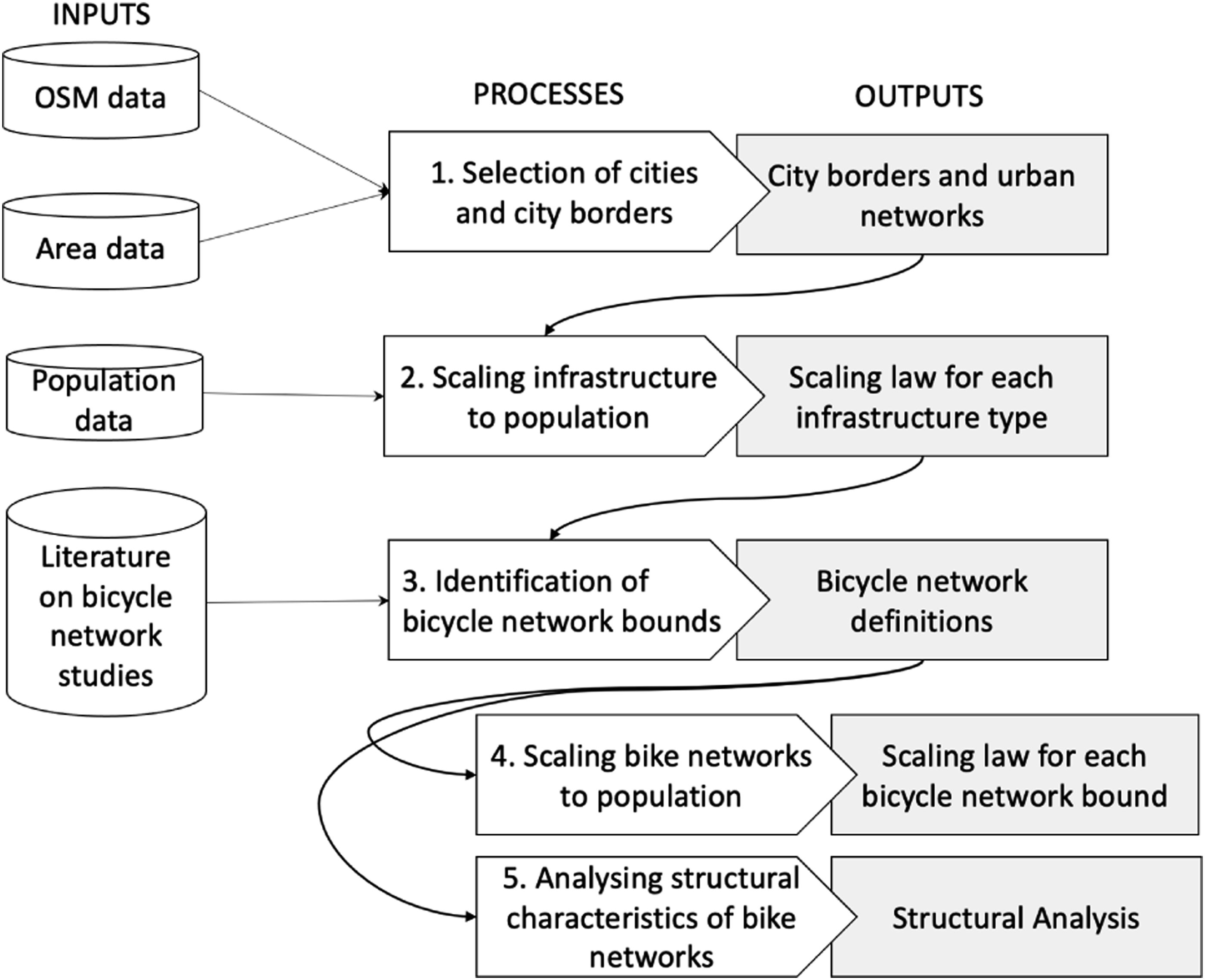

Selected cities and city boundaries

We analyse bicycle networks in different cities. The sample composition is built in such a way to include cities from as many different continents, with small to large population scale and with all ranges of bicycle mode share (from 1 to 46%). We decide to use Open Street Map (OSM) data due to its open accessibility, while being aware of the potential data quality issues. In fact, Ferster et al. (2019) report observing inconsistent tagging of bicycle infrastructure types. On the other hand, they also report that OSM can be more updated than municipality records, given the higher frequency with which ‘the crowd’ contributes to updating the OSM compared to the city releasing updated data.

The sample selection was constrained to the availability of OSM data; we only selected countries with OSM network data exceeding 80% completeness Barrington-Leigh and Millard-Ball (2017) and with medium to high levels of bicycle ownership Oke et al. (2015). We believe that country OSM data is a good representation for cities if we are to consider national level policies in provision of infrastructure. However, some cities could be more complete than the country they are part of because of external events (e.g. like Covid is highlighting in Paris) and this selection criteria may exclude interesting cities from the analysis. This choice inevitably biases the city sample towards more developed countries for which these data are digitally available, leading to more similar typologies of street patterns among cities Louf and Barthelemy (2014). Moreover, in order to have a representative sample of cities with high bicycle mode share, the sample has an over-representation of the dutch cities, which are typically of small size (population of maximum 1 million inhabitants). To address this concern, we included a sufficient number of small-sized cities that have lower cycling rates than in the Netherlands, in order to not bias the sample with small-sized cities that only represent a high cycling mode share level. In light of the selection method explained above, city selection in this paper could be biased, and further research that helps in identifying less biased selection would be extremely valuable. The list of cities under analysis is reported, for lack of space, in Table S1 in the Supplementary material.

Defining the city boundaries is a non trivial task. Cities are not well-defined entities that can be described by administrative boundaries, functional economic areas, urban form, and presence and movement of people Rybski et al. (2019). Cities, differently to urban centres, have an administrative and cultural identity that influences bicycle network investments and travel behaviour. Instead, urban centres are made of dense territories which may be composed of different local political administrations. We selected city boundaries based on Nominatim OSM (2021a) (a tool to search OSM data by name) administrative boundaries. If more than one boundary is available for a city we always avoid city metropolitan boundaries which, in most cases, incorporate scarcely populated areas and more than one local administration. After extracting municipality borders, we use https://www.citypopulation.de/website as a visual reference to extract the corresponding population and area information. This ensures that the population matches the selected city boundaries. Area, population and bicycle mode share information per city is reported in the Supplementary material (see section city data).

Scaling infrastructure to population

We extract urban network, of the selected city boundaries, from the OpenStreetMap (OSM) project via OSMnx Boeing (2017) we compute the respective kilometre length of each infrastructure type (e.g. primary roada, secondary road and pedestrian street) for each city. Next, we employ a log-normal analysis using the Bayesian information criterion (BIC) to model a power-law distribution for the kilometres of infrastructure and population, and examine the scaling exponents. For further details on the BIC and its suitability for this type of analysis, please refer to Leitão et al. (2016).

Identification of bicycle network bounds

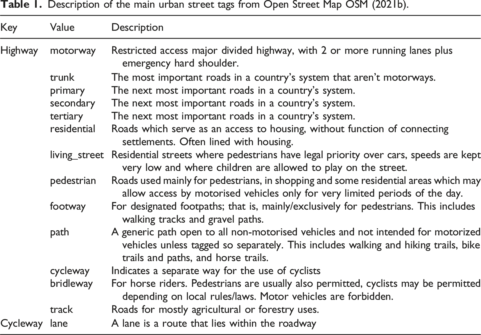
Combining the results of the scaling laws with best practices identified in the literature we define four bicycle network definitions (bounds). To define bicycle networks, we use infrastructure types used in OSM. In Table 1 we report the keys, values and definitions of the main infrastructure types, as defined on OSM. The remainder of the paper refers to these definitions when describing types of street infrastructure.

Table 1.

Description of the main urban street tags from Open Street Map OSM (2021b).

Key	Value	Description
Highway	motorway	Restricted access major divided highway, with 2 or more running lanes plus emergency hard shoulder.
	trunk	The most important roads in a country’s system that aren’t motorways.
	primary	The next most important roads in a country’s system.
	secondary	The next most important roads in a country’s system.
	tertiary	The next most important roads in a country’s system.
	residential	Roads which serve as an access to housing, without function of connecting settlements. Often lined with housing.
	living_street	Residential streets where pedestrians have legal priority over cars, speeds are kept very low and where children are allowed to play on the street.
	pedestrian	Roads used mainly for pedestrians, in shopping and some residential areas which may allow access by motorised vehicles only for very limited periods of the day.
	footway	For designated footpaths; that is, mainly/exclusively for pedestrians. This includes walking tracks and gravel paths.
	path	A generic path open to all non-motorised vehicles and not intended for motorized vehicles unless tagged so separately. This includes walking and hiking trails, bike trails and paths, and horse trails.
	cycleway	Indicates a separate way for the use of cyclists
	bridleway	For horse riders. Pedestrians are usually also permitted, cyclists may be permitted depending on local rules/laws. Motor vehicles are forbidden.
	track	Roads for mostly agricultural or forestry uses.
Cycleway	lane	A lane is a route that lies within the roadway

Since there is no universally accepted definition of a bicycle network, we systematically estimate upper and lower bound definitions and use them as candidate definitions for our network analysis. Driven by previous studies and the ability of employing these definitions to any city worldwide, we identify four definitions of bicycle networks. The network definitions are step-wise incremental, thus the lower bound is the smallest in size and the upper bound network is the largest, as it includes all the streets included in the previous definitions. Going from the most physically separated from vehicular traffic (widely considered as the safest) to the least segregated (also considered the least safe¹ to cycle on) we label them lower bound, medium-lower bound, medium-upper bound and upper bound.

• The lower bound network is made of bicycle tracks that are physically separated from vehicular traffic, living streets with very low speed limits, and recreational paths. Studies of Szell (2018); Orozco et al. (2020); Nello-Deakin (2019) use only bicycle streets that are physically separated (protected) from vehicular traffic because of their higher safety levels. In our definition of lower bound, in addition to the separated bicycle streets, we also include living streets and paths which can be considered equally safe and comfortable because active modes have priority over cars OSM (2021b). Thus, the lower bound definition consists of only protected bicycle streets.

• We define the medium-lower bound network as a combination of protected and unprotected bicycle streets because unprotected bicycle lanes (considered less safe) are mostly present in Western countries with the strongest car culture Szell (2018). Note that bike lanes are visually (not necessarily physically) separated form vehicular traffic.

• The medium-upper bound extends the previous definition by adding residential streets. These are streets for local traffic which typically have low volumes of through movement. During the COVID-19 pandemic, some cities have transformed these into slow streets WHO (2020). This motivates the definition of a bicycle network that assumes all residential streets to be suitable for cycling.

• Finally, the upper bound network includes all streets where cycling is not prohibited by law, which encapsulates the broad definitions of bicycle networks used in literature Wu et al. (2021); Yen et al. (2021).

For reproducibility purposes, the OSM queries used to define the four bicycle networks are reported in Table S3 in the Supplementary material.

Note that the bikeability² and safety of all bicycle streets is generally dependent on the city and its culture. This is especially true for non–bicycle-separated streets, for example, residential streets, bike lanes (with no physical separation) and all vehicular roads where cycling is allowed. However, it is reasonable to assume that the lower bound network is the safest bicycle network in all countries, whereas the upper bound also includes the least safe streets.

The taxonomy of bicycle networks is schematically visualised and explained in Figure 3. The four networks are step-wise incremental since all streets included in the lower bound network are also present in the upper bound networks. To illustrate how the bicycle network bounds are different in structure and extension, in Figure S2 in the Supplementary material we visualise the four bicycle networks for a small (Delft) and large (Rome) city.

Figure 3.

Taxonomy of bicycle network types.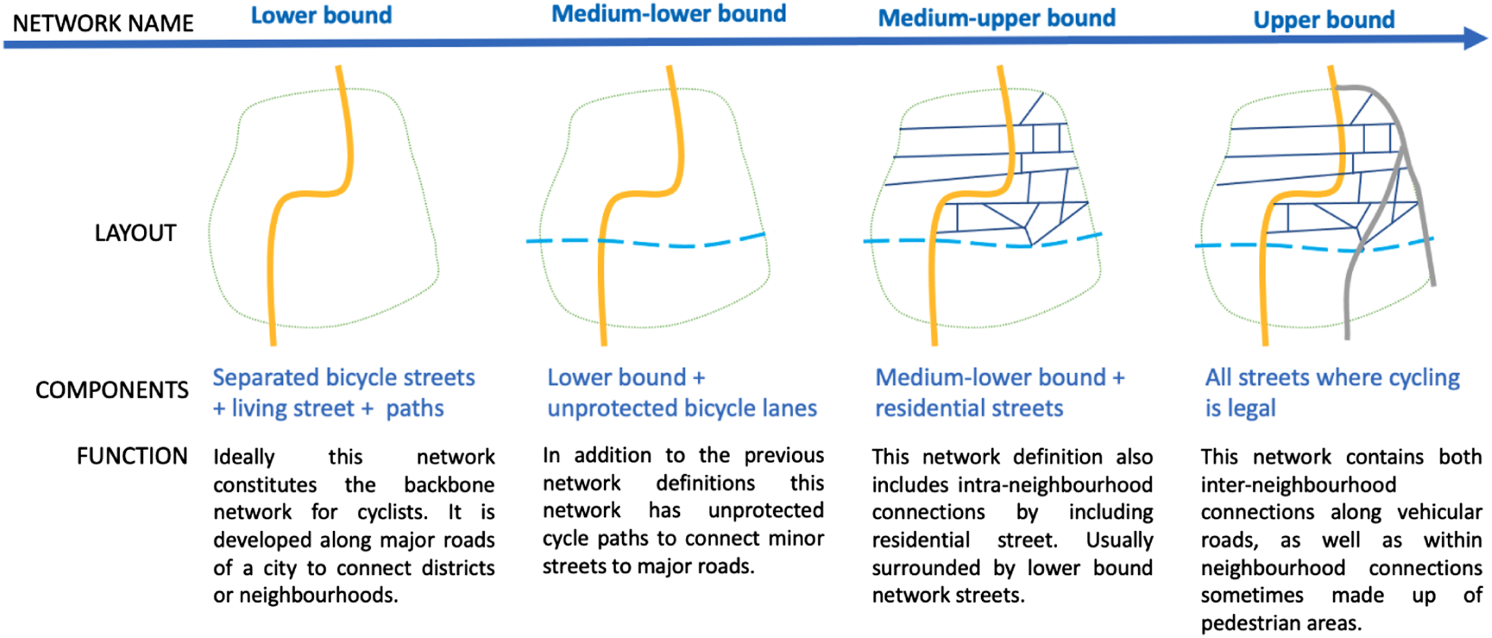

Scaling bike networks to population

Similarly to step 2, we use the Bayesian information criterion (BIC) to fit a power-law distribution. In this step we analyse how the kilometres of the bicycle network bounds scale to population.

Structural analysis and network measures

As illustrated in Figure 3, there are disparities in the extent to which a bicycle network spans a city. To provide an information basis for policymakers to direct infrastructure investments, it is imperative to study network structural characteristics more systematically. Most structural characteristics are correlated to travel behaviour and can be influenced by policymakers to incentivise bicycle use. A pioneering study on bicycle network analysis identified size, fragmentation, directness, density and connectivity as macroscopic factors to measure bicycle network quality Schoner and Levinson (2014). Besides these characteristics, we also include granularity – measured as average street length – due to its wide adoption in urban street network analysis studies Boeing (2021); Yen et al. (2021). These network measures are a good proxy for information about land use and transportation system (i.e. cost of travel) of the city Van Wee et al. (2013); Schoner and Levinson (2014); Kamel and Sayed (2021). The measurements are computed with standard (python) libraries in the network community such as NetworkX and OSMnx. A definition of each measurement is reported hereafter.

Size, or extension, of urban bicycle networks measures the total kilometre length of the network. To measure a specific infrastructure type (e.g. residential streets) the relative size is measured as the ratio of that infrastructure type over the extension of the whole network. The extension, in absolute and relative terms, shows investment decisions of cities and allows to analyse space distribution between transport modes. Previous studies have found positive relationships between the size of a city’s bicycle facility network and its bicycle commute share Dill and Carr (2003); Buehler and Pucher (2011); Parkin et al. (2007).

Fragmentation, as defined in this work, measures the number of the connected components of a network and their size distribution. A network made of only one connected component, implies that there is a path between every pair of nodes in the network. Whereas, networks made of many connected components result in more isolated parts which do not connect to all nodes of the network. The size of a connected component is computed as ratio of the kilometre extension of the connected component over the total extension of the network. Most cities have one giant connected component that makes up the car, pedestrian, and rail network, whereas the bicycle street network is often fragmented into many connected components Orozco et al. (2020). Having either a few medium sized components or one dominant component facilitates bicycling, but excessive fragmentation with small fragments should be avoided Schoner and Levinson (2014). Moreover, fragmentation of the network can constitute a resistance to cycling by reducing safety and comfort.

Granularity of an urban street network measures block size which is the elementary component of an urban map. The average street length is a proxy to measure city granularity. Previous empirical results have shown that this indicator has positive relationship with levels of economic vitality for cities Long and Huang (2019). Fine-grained urban areas are also naturally more attractive for active modes because there are more locations to stop along the way, than in coarse-grained urban areas. We study how network granularity changes over the bicycle network definitions. Note that the underlying street network stays the same, so the physical street layer has always the same granularity, however the bicycle networks have different granularity depending on which components of the street network are included in the definition. Cyclists experience higher or lower granularity depending on the streets they deem bikeable.

Directness, the inverse of circuity, measures the ratio of euclidean (straight line) to street distance. This network characteristic describes the directness and the efficiency of transportation networks. Cyclists are affected from the directness of their routes, so policies that make bicycle trips more direct and efficient will increase adoption of cycling as a mode of transportation Rietveld and Daniel (2004).

Network density provides information on the land use of a city and can be measured in a number of ways. We measure it as intersection density (intersections/km2). Density has been identified as the most influential factor for bicycle commuting among network characteristics in a study across US cities Schoner and Levinson (2014). That study concluded that: ‘cities hoping to maximise the impacts of their bicycle infrastructure investments should first densify their bicycle network before expanding its breadth’. Studies on the relationship between the built environment and travel have identified that residents of high-density neighbourhoods use the bicycle more often Van de Coevering (2021) and that a change in the density factor score of one standard deviation corresponds to a 77% increase in rates of bicycle commuting Schoner and Levinson (2014).

Connectivity describes how well locations (nodes) are connected via network links and can be measured in a variety of ways. In this work, similar to previous urban studies Boeing (2017, 2021); Schoner and Levinson (2014), connectivity is measured in terms of streets³ per node, proportion of streets per node and clustering coefficient of nodes. These characteristics, respectively, shed light on the average node level connectivity, distribution of node level connectivity and neighbourhood level connectivity. The average streets per node measures the average number of physical streets that emanate from each node (i.e. intersection or dead-end). It is the street equivalent of the network’s average node degree. The clustering coefficient of a node is the ratio of the number of edges between its neighbours to the maximum possible number of edges that could exist between these neighbours. The average clustering coefficient is the mean over all nodes of the network and expresses how robustly the neighbourhood of some node is linked together Kamel and Sayed (2021). The proportion of streets per node describes the type and distribution of node level connectivity. Empirical results in previous studies have shown a positive and significant relation between connectivity and bicycle commute share Schoner and Levinson (2014).

To test if the network measures are statistically different over the four bicycle network bounds (statistically speaking these are groups), we need a repeated measures non-parametric test, because the groups are dependent and not normally distributed. We use the non-parametric Friedman test, similar to the parametric repeated measures ANOVA, used to detect differences in treatments across multiple test attempts. If the H₀ hypothesis of the Friedman’s test is rejected, we conduct a post hoc analysis to identify among which bike network bound there is a statistical difference. The post hoc analysis in this case requires a Wilcoxon test with Bonferroni adjustment because we are making multiple comparisons, which makes it more likely that Type I error appears.

Finally, to assess the different types of network definitions, we calculate relative change in network measurements as

I_{i} = \frac{| C_{i} - C_{i + 1} |}{C_{i}} \times 100

(1)

where C_i is the characteristic (e.g. density) in i − th network ( the medium-upper bound network) and C_i+1 is the same characteristic computed for the following network definition (so in this case the upper bound network).

Empirical analysis and results

This section presents results of the scaling analysis and of the structural analysis of bicycle networks. In particular, sections Scaling infrastructure type to population and Scaling bicycle network kilometres to population investigate on research question 1 and the subsequent sections investigate on research question 2.

Scaling infrastructure type to population

To test if scaling relations (i.e. Y = αX^β) hold between individual types of road infrastructure length and city population we conducted a log-normal analysis using the Bayesian information criterion (BIC). When comparing the scaling relation of bicycle infrastructure in cities, it’s crucial to consider that different cities may be at different stages of development and have varying amounts of cycleway infrastructure, making it important to establish different network bounds for accurate comparisons. Figure 4 reports β, estimation error, p-value, BIC difference between the maximum-likelihood of the log-normal model with the corresponding model where β = 1 (methodology and code extracted from Leitão et al. (2016)). If ΔBIC > 6 the model with β ≠ 1 provides a sufficiently better description of the data.

Figure 4.

Scaling of urban infrastructure types. Relation between total kilometres of infrastructure and population of the corresponding 47 cities. The table groups infrastructure types into public transport (green), active mode (orange), and vehicular infrastructure (grey). The plot on the right uses shades of those three colours to visualise some relations. Lines are drawn using the β values obtained via a log-normal fit analysis with Bayesian Information Criteria with required successes set to 10 (see Leitão et al. (2016)).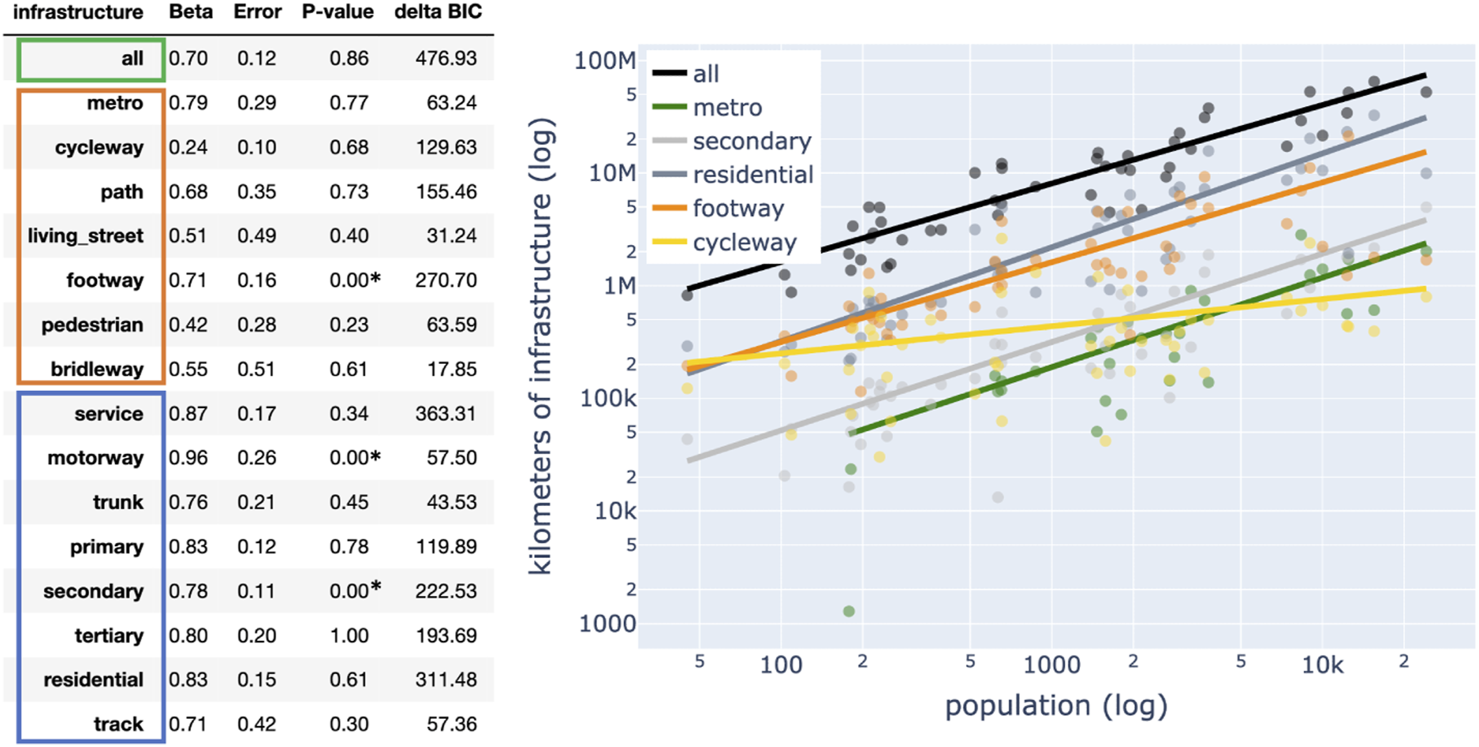

The analysis confirms that the size of all road infrastructure scales sublinearly with population, meaning that cities are economies of scale and are efficient in providing road infrastructure. This is in line with the findings from urban scaling law studies Bettencourt (2013). Zooming into the specific infrastructure types, Figure 4 shows that, the metro infrastructure scales sublinearly with β = 0.79, the car infrastructure scales sublinearly with an exponent β ∈ [0.71 − 0.96], and the cycling and pedestrian infrastructure scales sublinearly but more slowly; β ∈ [0.22 − 0.76]. The p-value quantifies whether the fluctuations in the data are compatible with the expected fluctuations from the model and whether the residuals are uncorrelated (see paper Leitão et al. (2016) for more info). In case of p-value $< 0.05$ the model is rejected and the corresponding entry in table of Figure 4 is marked with an asterisk. Although population size is not the only influencing factor of active mode infrastructure growth, our analysis shows statistical evidence that larger cities provide overall less active mode infrastructure per capita. In particular, cycleway infrastructure grows 70% slower than the average road infrastructure.

Scaling bicycle network kilometres to population

The previous section has shown how the scaling rate changes as we look at different infrastructure types. Thus, depending on which infrastructure type is included in the bicycle network definition, one can observe different scaling relations between bicycle network etension and city size. From this section onwards we will analyse bicycle networks defined in section.

In absolute terms, the size of the bicycle network increases as the definition includes more infrastructure types by definition. All bicycle network types have statistically different sizes in terms of kilometres of network. In particular adding unprotected bike lanes increases the average network size by 1.75%, adding residential streets and streets where cycling is not prohibited respectively increases the network size by 228.12% and 134.04%.

The four types of bicycle networks scale at a different rate to population size. The lower and medium-lower bound in Figure 5 scale half as slower than the medium-upper and upper bound. The inclusion of non-dedicated bicycle street (as in the definition of medium-upper and upper bound networks) increases the scaling rate, between kilometres of bicycle infrastructure and city size, from β; 0.4 to β; 0.7. So, the fastest way for a city to increase kilometres of bike network per person is to increase safety of residential streets and streets where cycling is not prohibited (if they are not bicycle friendly already), for instance by reducing speed limits.

Figure 5.

Size of the bicycle networks. Scaling of the four types of bicycle network kilometres to population. Data for 47 cities extracted from OSM in 2020. Lines are drawn using the β values obtained via a log-normal fit analysis with Bayesian Information Criteria (see Leitão et al. (2016)).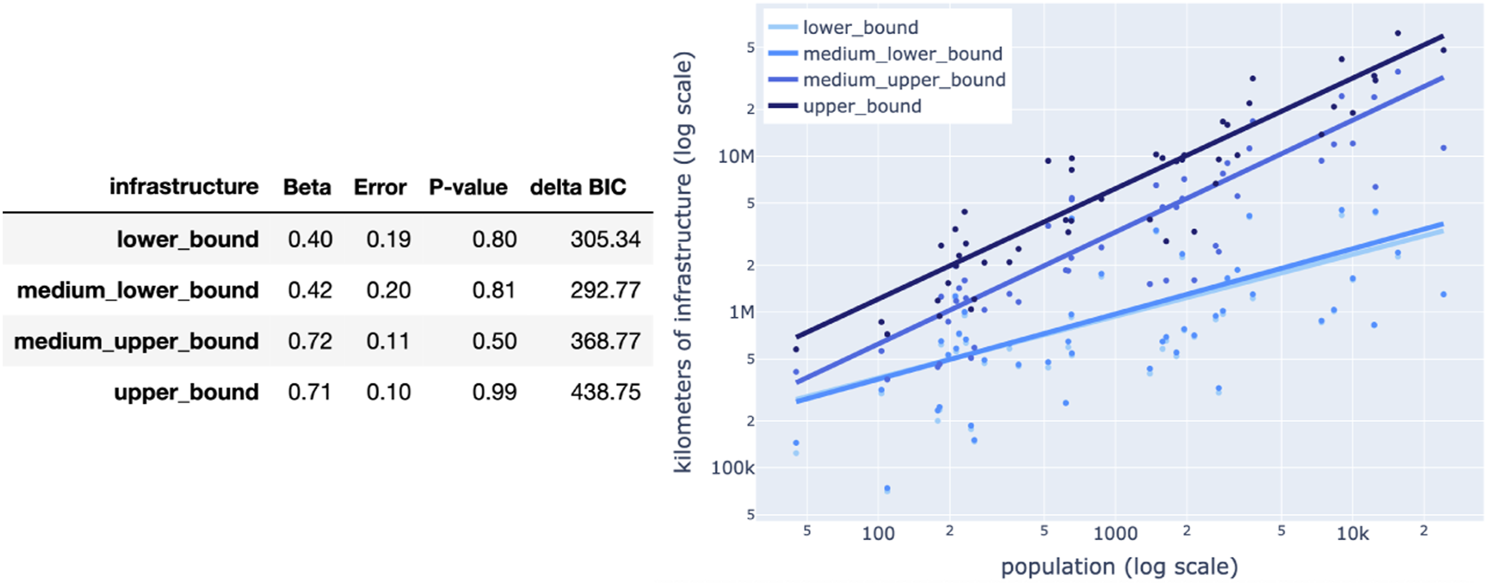

In conclusion, we see that different bike network bounds scale differently with population. It all depends on the infrastructure types included in the bicycle network definitions. In the next sections we study the aggregated structural characteristics of the four candidate definitions of bicycle networks.

Fragmentation

The number of connected components is significantly different depending on the type of bicycle network, as is shown by applying a Friedman test. A post hoc analysis with Wilcoxon signed-rank tests, with a Bonferroni correction applied (pvalue = 0.083), showed significant differences between all networks except between the lower bound and the medium-upper bound and between the medium-lower bound and medium-upper bound. Thus each network definition has on average a different number of connected components, except for the medium-upper bound which has a similar distribution to the other lower bound networks.

By analysing the number of connected components of the four bicycle network types, we see in Figure 6(a) that as the bike network definition includes more infrastructure types (different shades of blue in Figure 6(a)) the number of connected components decreases. An exception to this is the addition of residential streets (medium-upper bound). Namely, the slope of the fitted line in the medium-upper bound is larger than the slope of the lower bound, meaning that for cities with a small population the residential streets behave as a ‘connector’ (since the number of connected components is less than the connected component in the lower bound), and for big cities they behave as ‘separators’ (since the number of connected components is higher than the connected component in the lower bound).

Figure 6.

Connected components of the bicycle networks. (a) Number of connected components in relation to bicycle network definition and city size. (b) The connected component size distribution of 47 cities over lower, medium-lower, medium-upper, and upper bound bicycle network types. The abscissa is constrained to 10 connected components; the connected component of rank 1 is the largest connected component, rank 2 is the second largest connected component and so on. The ordinate shows the relative size of each connected component with respect to the total network kilometres. For a given city, the sum of all relative sizes over all connected components is equal to one.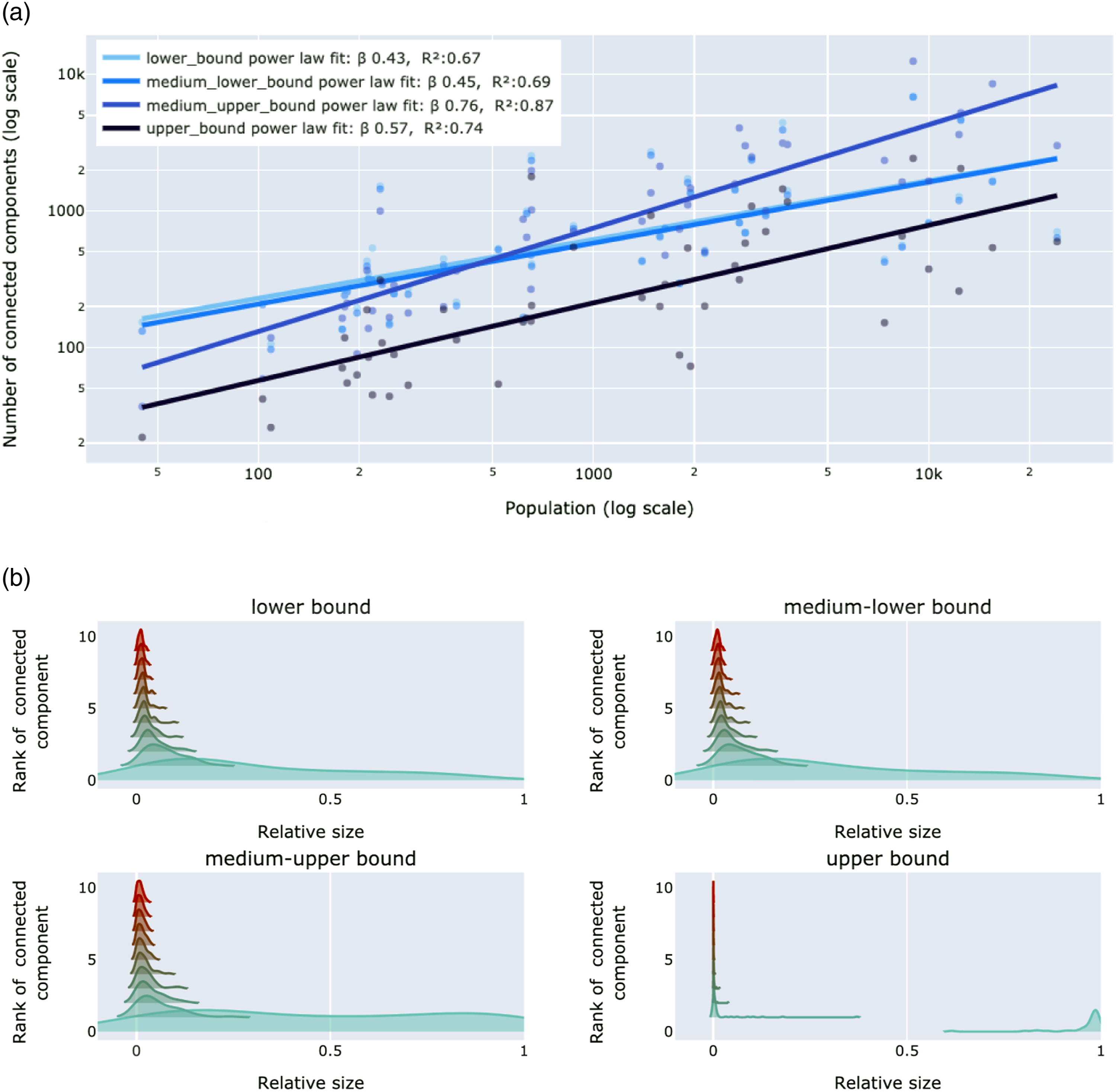

Figure 6(b) shows the difference in the connected component size distribution of the four bicycle networks. In the lower bound network the largest connected components (i.e. rank of connected component = 1) are small (average relative size is below 0.5), and the following components are of medium size (relative size of 0.2 to 0.1). Moving towards the upper bound network the networks have the largest connected components of relative size close to 1 and the other components of negligible small size. From Figure 6(b) we note that the addition of residential streets does not change the component size distribution, though Figure 6(a) shows that residential streets do change the total number of connected components. The real difference in component size distribution is given by adding all streets where cycling is not forbidden. This results in the upper bound network being the least fragmented network.

Granularity

Figure 7(a) shows that city granularity significantly decreases in value and dispersion as the bicycle network definition broadens to include non-dedicated bicycle streets. This indicates that the broader bicycle network definition has more homogeneous street segment lengths between cities compared to the lower bound bicycle network. The average street length of the lower bound network varies from maximum of 311 m in Bogota to a minimum of 57 m in Helsinki. Whereas the average street length of the upper bound network varies from maximum of 223 m in Shanghai to a minimum of 47 m in Helsinki. This empirically confirms that the lower bound bicycle network can be considered as the safe backbone network for cycling, with a few long and direct streets (with not many branches), and the other networks as an expansion to it, with more branches and intersections.

Figure 7.

Structural characteristics of bicycle networks. (a) Average street length, (b) Average street circuity, (c) Average intersection density, (d) Average streets per node, (e) Clustering coefficient, (f) Proportion of streets per nodes.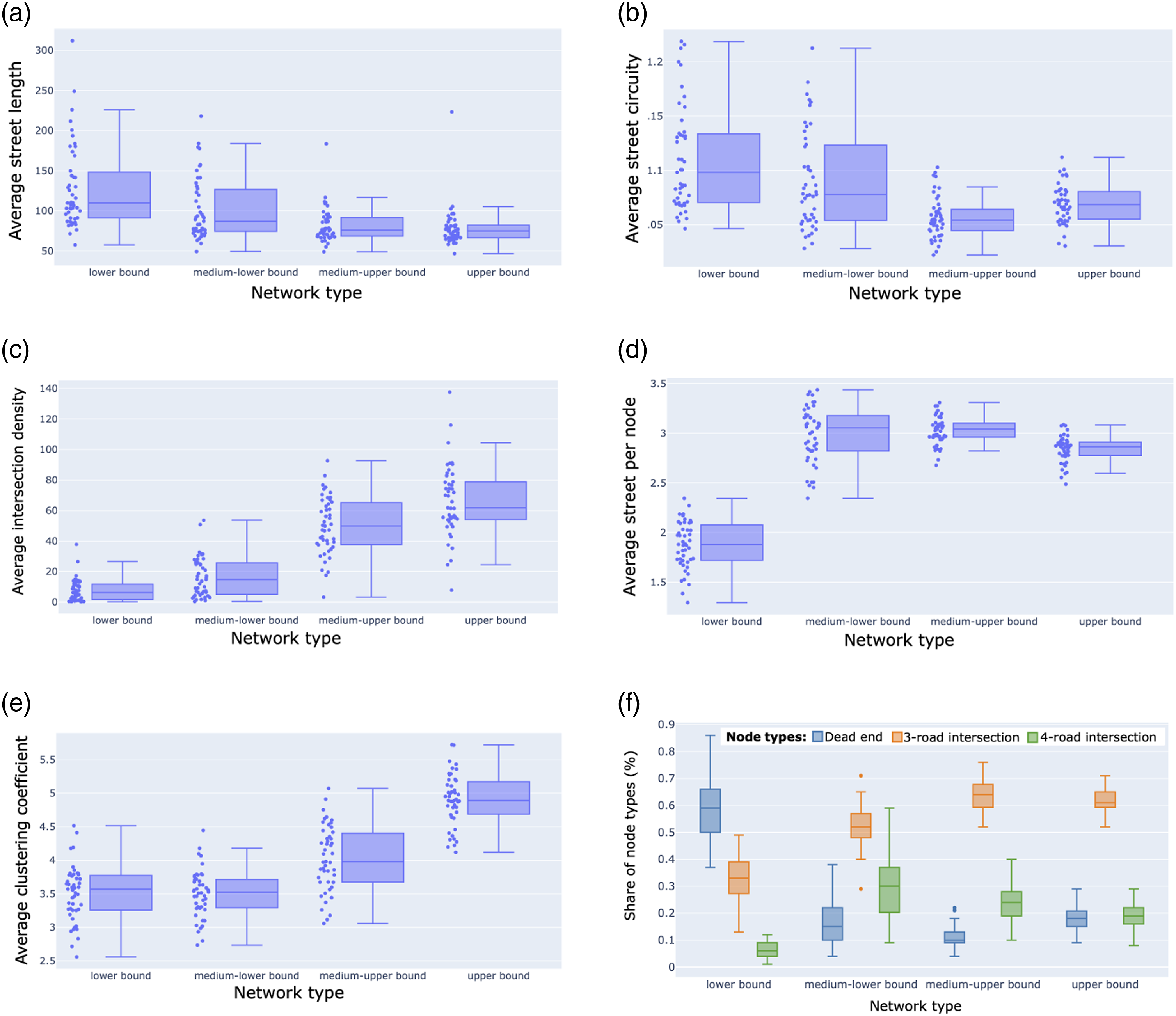

The Friedman test showed a significant difference in granularity depending on the type of bicycle network. The median average street length for the lower, medium-lower, medium-upper and upper bound network are 109, 87, 76 and 74, respectively. A post hoc analysis with Wilcoxon signed-rank tests, with a Bonferroni correction applied (pvalue = 0.083), showed significant differences between all networks.

Directness

The average street circuity decreases in value and dispersion as the bicycle network definition broadens as shown in Figure 7(b). The Friedman test showed a significant difference in the average circuity depending on the type of bicycle network. The median circuity for the lower, medium-lower, medium-upper and upper bound network are 1.098, 1.077, 1.054 and 1.068, respectively. The Wilcoxon signed-rank tests (with a Bonferroni correction) showed significant differences between all networks except between the medium-lower and the upper bound.

The average street circuity of the bicycle networks are higher than the circuity of street networks of many world sub regions Boeing (2021). For example, Europe has a street circuity between 1.065 and 1.059 according to Boeing (2021). Our analysis, instead, shows that Fukuoka, Boston and Rome have the circuity of 1.20 and Rotterdam of 1.04; these are the highest and lowest circuity values for the lower bound network.

The network with lowest circuity is the medium-upper bound, which shows the convenience of adding residential roads to the bicycle network definition. Residential streets create within neighbourhood connections. For this reason by including them in the bike network definition they result in more direct routes that do not meander around residential areas but cut through them. We notice that circuity increases from the medium-upper to the upper bound network, one explanation is that the upper bound network does not only add within neighbourhood connections, it adds all streets where cycling is allowed. The latter results to be more circuitous than the residential streets.

Density

Figure 7(c) reports intersection density values for the different bicycle network definitions across 47 cities. Data shows that the lower bound network has significantly lower densities, in terms of number of intersections over square km, compared to the other networks. The Friedman test showed a significant difference in average intersection density among the different bicycle networks. The median density for the lower, medium-lower, medium-upper and upper bound network are 6.1, 14.7, 49.8 and 61.8, respectively. These densities are much higher than the vertex densities (average 1.55 vertex/km²) of bicycle networks reported in Schoner and Levinson (2014). The reason could be linked to the choice of the cities in the two studies. Our study selected cities over four continents but still has a large representation of European cities, while the other study was entirely focused on US cities.

The Wilcoxon signed-rank tests (with a Bonferroni correction) showed significant differences between all networks. This confirms that the network becomes more dense of intersections as more infrastructure types are added to the network. The biggest increase in density is between the medium-lower bound and the medium-upper bound. This is interesting because it highlights the crucial role of residential streets in densifying the network.

Connectivity

Empirical results in Figure 7(d) show that the lower bound network has a significantly lower number of streets per node. The Friedman test showed a significant difference in values and the Wilcoxon signed-rank tests (with a Bonferroni correction) showed significant differences between all networks except medium-lower and medium-upper bound. The medium bound networks have a similar amount of streets per network, showing that residential streets do not increase the average node connectivity. Interestingly it is not the upper bound network that has the highest number of streets per node. Our interpretation is that the upper bound network, although it has the largest network in size, it does not connect the streets to existing nodes. It most likely adds new nodes, as well as street, components to the network.

Figure 7(e) shows that the bicycle network with the highest clustering coefficient is the upper bound meaning that network is the most clustered and connected at the neighbourhood level. The Friedman test showed a significant difference in values. The post hoc Wilcoxon signed-rank tests did not show significant difference between the lower and medium-upper bound and the medium-lower and the medium-upper bound network, indicating that residential streets do not play a crucial role on the neighbourhood level connectivity. For the upper bound, instead, the clustering coefficient significantly increased with the addition of all streets where cycling is allowed. The reader should note that although the clustering coefficient is a commonly used metric for assessing networks, the resilience of a network requires more complex analysis on clustering vulnerability.

Results in Figure 7(f) highlight a big difference between the lower bound network and the others. The lower bound network is characterised by a very big share of dead-ends (64%), lower share of 3-way intersections (33%) and an even lower share of 4-way intersections (6%). The large proportion of dead-ends in the lower bound bicycle network makes clear that this type of bicycle network has many loose ends, resulting in a less connected network. This is very different from the average vehicular street network. Boeing (2017) has shown that the average USA urban agglomeration is characterised by a preponderance of three-way intersections. The typical urbanised area has many three-way intersections (59%), fewer dead-ends (21%) and even fewer four-way intersections (18%). The medium-upper bound bicycle network, instead, has very few dead ends (10%), many 3-way intersections (64%) and a few four-way intersections (24%). Thus adding residential streets to the bicycle network results in more 3- and 4-way intersections.

Relation between indicators

This section explains how the previous indicators are related and how they support or contradict different findings. This will be discussed through the example of Delft and Rome. The summary of network indicators for these two cities (across the four bicycle networks) is reported in Figure S3, which for lack of space is in the Supplementary material.

As the total street length increases also intersection density seems to increase. However, the relation is dependent on how the new streets are added. If streets are added as disconnected components they will increase the node density but not the intersection density. Whereas if the new streets are linked to the existing network, their addition increases the intersection density. Thus, the increase in total street length has a higher impact on intersection density if the number of network components does not increase. This is visible in Figure S3 between the medium-lower and medium-higher bound networks. Rome has a bigger increase in total street length than Delft; however, it also has a much higher increase in number of components. The result is that Delft’s medium-upper bound network has a much higher intersection density.

As we go from the lower to the upper bound network the average street length decreases. Previous researches have shown that longer links are safer to travel given that there are less discontinuities and hindrances Kamel and Sayed (2021). This reinforces our definition of lower bound network being the safest, and upper bound network being the least safe, not only for the infrastructure type but because of the higher exposure to road discontinuities. The advantage of lower average street length is the lower average circuity of an edge, which leads to more direct routes.

Finally, the clustering coefficient indicator and the average street per node show two different aspects of network connectivity. In fact, the clustering coefficient relates to the average node degree and not so much to streets per node indicator. The average streets per node is based on the number of physical streets and not the network edges (in practice there can be one physical street but two network edges, one for each riding direction). By using the average street per node indicator, we look at the connectivity of an undirected representation of the network; reasonable if we assume that it is common that cyclists use a bike lane in both directions Viero (2020). To measure connectivity and robustness of the directed network the clustering coefficient (or the average node degree) are more suitable.

Implications for practice

The findings of this paper are of interest for researchers and policymakers. The type of bicycle network a researcher analyses in her study has implications on the study results; for example, the lower bound network turned out to be the most fragmented whereas the upper bound network is significantly more connected. Policymakers can use the average structural performance of bicycle networks as benchmark values to assess existing urban networks or plan urban development elsewhere. Moreover, policymakers can identify the type of bicycle network that meets their policy objective and determine the traffic calming measures needed to make the network suitable for different user groups. In the following, we illustrate a simplified framework of how policymakers can use the outcome of our analysis. For additional details on the network design the reader may refer to CROW (2017).

1. A city sets its objectives regarding the bicycle network based on the desired network characteristics. Network requirements are defined in terms of size, fragmentation, granularity, directness, density and connectivity according to the city context.

2. Once the objectives have been set, the network structural indicators should be computed over the four bicycle network definitions.

3. Then, the city can proceed to identify which (or a combination) of the four bicycle networks fits all the determined structural requirements⁴ (as defined in step 1.).

4. Finally, the city determines what needs to be done to make all roads (e.g. in terms of traffic regulations) included in the identified (at step 3) network definition truly bikeable. This analysis can be carried out per user group, referring to the four user groups proposed by Geller (2009).

In reality the decision process of developing a bike network is more complex, as planners do not only consider the structural characteristics, but also dynamic variables like traffic volume.

Discussion and conclusions

In this study, we tested the scaling relation between kilometre of infrastructure and city population to reveal the different growth rates of road infrastructure. In addition, we systematically defined four types of bicycle networks and conducted statistical tests to investigate the structural characteristics of bicycle network worldwide. The following sections elaborate on the results and draw conclusions by answering the questions stated in the introduction.

As larger cities build less infrastructure per capita, how do the different infrastructure types scale with city size and how is the scaling relation of bicycle networks affected?

Empirical results show that all types of infrastructure scale sublinearly. Although the types of infrastructure dedicated to active modes (cycleway, living street and pedestrian) scale sublinearly, they scale slower than non-active mode infrastructure. Namely, we observed that cities that have double the population appear to have 24% more kilometres of bicycle dedicated infrastructure but around 80% more primary, secondary and tertiary car road infrastructure. This provides a striking insight on cities’ investment decisions. Cities have been defined as efficient places due to their economies of scale in infrastructure. Our results confirm this efficiency but point out at the less liveable and sustainable side of large cities. Larger cities systematically invest less in bicycle dedicated infrastructure.

We observe that cities that have better biking conditions also have traffic norms that make car roads also bikeable. Since car roads can be used by bikes, but not vice versa, cities can compensate for the difference in bicycle infrastructure per capita by making multi-modal use of the streets safe for both modes, and across user groups. This is supported by our results showing that the scaling relation between kilometres of bicycle network and population is faster if the bike network includes multi-modal streets.

Following the logic of the built environment influencing attitude and ultimately travel behaviour, there is a risk that larger cities provide less bicycle friendly environment which may results in less positive attitude towards the bike. This risk is smaller if the bicycle network (used by most user groups) is made of more than just the separated bicycle tracks. We note that, among urban areas, large cities are places with larger disparity between active and non-active mode infrastructure supply. Sustainable and active mode challenges in urban mobility seem to lie in the large cities.

As different definitions of bicycle network exist, how can we provide evidence-based knowledge on the structural differences and similarities of bicycle networks worldwide?

We have designed a multi-city and multi-definition analysis of bicycle networks. This allowed us to numerically analyse the structural differences between bicycle networks and build evidence-based knowledge on unified definitions of bicycle networks. Our results show that network characteristics significantly change between different bicycle network definitions. Almost all characteristics are significantly different over the four network definitions. The lower bound network is significantly less extended, dense and connected and more coarse-grained and circuitous. This confirms that the four bicycle networks identified in this study are structurally different. It also implies that the choice of the bicycle network definition is a fundamental one and has consequences on accessibility, equity and safety evaluations of a city. For example, it can result in opposite accessibility evaluations if one were to compare accessibility per mode based on the upper instead of the lower bound network.

Studies have shown the fragmented and underdeveloped nature of many bicycle networks worldwide and advise significantly extending the protected bicycle lanes to create complete bicycle networks. For example, in cities like Seville, a fully protected bike lane network was feasible and materialised through consistent government funding into active modes of transportation Marqués and Hernández-Herrador (2017). Although we are in favour of spatial equity and justice between modes, and in reducing barriers to cycling, we challenge this type of notion based on the idea that a fully separated bicycle network is often not a feasible outcome. As an example, in cities that prioritise cycling, there are many segregated bike paths but also many shared streets where bikes go together with pedestrians and cars (think of historical city centre areas or residential areas). In some cases, bike networks can even be designed depending on the use of streets by different demographics, thus challenging municipalities to address multiple needs by developing protected, segregated or shared spaces for biking and other mixed land use. Driven by the question: ‘What type of streets make up a bicycle network’ we propose four definitions of bicycle networks, from the fully separated to the least (which includes also car streets where cycling is allowed) and systematically analyse their structural characteristics. This enables to evidence that the lower bound network is much more fragmented than the upper bound, both in number of connected components and size distribution of the components. This means that a policymaker aiming to reduce fragmentation of the bicycle street network can focus its efforts on making the infrastructure of the upper bound network (which is not dedicated exclusively to bicycles) truly bikeable, instead of expanding the size of the lower bound network.

Our empirical multi-city analysis showed the importance of residential streets which, by creating within neighbourhood connections, increase the network density, directness, connectivity and significantly extend its size. Including residential streets expands the total kilometres extension of more than 200%, reduces circuity by 4% and increases the density of intersections more than 700%. These are streets that already exist in the urban texture and are less expensive to transform into bicycle streets. In most city contexts, the physically-separated-from-traffic cycle tracks are not sufficient for people to reach their daily activity destinations by bicycle. However, the hierarchical combination of separated cycle tracks and residential streets (used by multiple modes) improves the network structure allowing cyclists to reach many more destinations within their neighbourhood.

Limitation of the methodology of scaling and power-law analysis

Many natural phenomena exhibit power-law distributions, in that when one quantity varies, the other also varies proportionally, based on the power of the first one. This pattern is observed in many physical and natural events, and analysing the parameters estimated from these distributions can reveal underlying processes. However, the selection of scale and magnitude of empirical data can impact the resulting parameter values Pickering et al. (1995). In social sciences, this becomes even more complex because power-laws occur through several policy decisions or demand-side adoption. Our analysis shows that bike infrastructure scales sub-linearly with population growth and is 70% slower than other road infrastructure. The exponent β, although biased by sample selection, informs us about specific decision-making aspects that have led to this infrastructure development: 1) bicycle ownership, 2) mode share, 3) systematic versus rapid share increase due to external events (like Covid), 4) level of data completeness and several other conceivable factors.

Although our results provide statistical evidence that the data is consistent with the scaling law model (as for the method proposed by Leitão et al. (2016)), the selection of cities may have biased the scaling parameter. To mitigate this limitation, a larger sample size of cities should be considered. However, caution must be taken to control for other factors when analysing a larger sample, as this could lead to inaccurate conclusions on a different scale or magnitude. To address this, we recommend investigating additional statistical evidence of non-linear relationships and low scaling parameters in cycleway infrastructure with larger samples.

Summary and final remarks

In conclusion, this analysis unravelled a disparity in the supply of active mode infrastructure, especially in big cities which systematically invest less in bicycle-dedicated infrastructure. Moreover, our finding suggests that city authorities could focus more on improving residential streets that already exist (with bicycle ad-hoc measures such as speed limit) rather than predominantly focussing on developing new separated or semi-separated bicycle streets. Depending on the legislation and the street design these can be very safe or unsafe roads for cyclists. Once a city has identified the definition of bicycle network it wants to refer to, it should take action to make it bikeable for its target user group. By doing so, planners can design cities not only to be exciting and efficient but also apt for sustainable mobility.

Supplemental Material

Supplemental Material - A multi-city study on structural characteristics of bicycle networks

Supplemental Material for A multi-city study on structural characteristics of bicycle networks by Giulia Reggiani, Trivik Verma, Winnie Daamen and Serge Hoogendoorn and Linda Theron in Environment and Planning B: Urban Analytics and City Science

Footnotes

Acknowledgements

The first author would like to thank Ruggiero Seccia for his coding assistance through various phases of the data analysis.

Author contributions

GR: Conceptualisation, Methodology, Formal analysis, Visualisations, Writing—original draft, Project administration. TV: Supervision, Writing—review \and editing. WD: Supervision, Writing—review. SH: Supervision, Methodology, Writing—review \and editing, Funding acquisition.

Declaration of conflicting interests

The author(s) declared no potential conflicts of interest with respect to the research, authorship, and/or publication of this article.

Funding

The author(s) disclosed receipt of the following financial support for the research, authorship, and/or publication of this article: This work was supported by the ALLEGRO project, which is financed by the European Research Council (Grant Agreement No. 669792) and the Amsterdam Institute for Advanced Metropolitan Solutions.

ORCID iDs

Giulia Reggiani

Trivik Verma

Supplemental material

Supplemental material for this article is available online.

Notes

Giulia Reggiani is a senior analyst in the sustainability decarbonisation domain, working for private and governmental parties. She did her PhD in the department of Transport and Planning, Delft University of Technology as part of the Allegro ERC project. She carried out her engineering bachelor and master studies, in la Sapienza University of Rome. Her research focused on structural properties of bicycle networks worldwide and on data driven methods for assessing bikeability. Her current interests lie in the broad domains of smart mobility, data analysis, sustainability and complex networks.

Trivik Verma is an Assistant Professor at Delft University of Technology. His research focusses on tackling challenges of urbanisation in an equitable and just manner. Specifically, he is using methods in spatial data science, complex network analyses and participatory mapping to develop computational tools for advancing the theories and practices of urban science.

Winnie Daamen is currently an Associate professor in the Department of Transport and Planning, Delft University of Technology, The Netherlands. Her research interests include theory, modeling, and simulation of active mode traffic (pedestrians, cyclists). The core of her expertise is in data collection, data analysis to get insight into traffic participant behavior and modeling these behaviors.

Serge Hoogendoorn was appointed Antonie van Leeuwenhoek professor Traffic Operations and Management in 2006. He has been the chair of the department Transport and Planning since 2018. He is currently (one of the five) Distinguished Professor of Smart Urban Mobility at Delft University of Technology. Hoogendoorn is the PI Mobility in the Institute of Advanced Metropolitan Solutions. His current research evolves around Smart Urban Mobility, with focal areas such as i) theory, modelling, and simulation of traffic and transportation networks, including cars, pedestrian, cyclists and novel public transport services; ii) development of methods for integrated management of these networks; iii) impact of uncertainty of travel behaviour and network operations; iv) impact of ICT on network flow operations, robustness and resilience, and v) urban data and its applications.

References

Barrington-Leigh

Millard-Ball

(2017) The world’s user-generated road map is more than 80% complete. PLoS ONE 12(8): 1–20.

Bettencourt

(2013) The origins of scaling in cities. Science 340(6139): 1438–1441.

Boeing

(2017) OSMnx: new methods for acquiring, constructing, analyzing, and visualizing complex street networks. Computers, Environment and Urban Systems 65: 126–139.

Boeing

(2021) Street network models and indicators for every urban area in the world. Geographical Analysis.

Buehler

Dill

(2016) Bikeway networks: a review of effects on cycling. Transport Reviews 36(1): 9–27.

Buehler

Pucher

(2011) Cycling to work in 90 large American cities: new evidence on the role of bike paths and lanes. Transportation 39(2): 409–432.

CROW (2017) Design Manual for Bicycle Traffic.

Dill

Carr

(2003) Bicycle commuting and facilities in major U.S. cities: if you build them, commuters will use them. Transportation Research Record 1828(1): 116–123.

Ferster

Fischer

Manaugh

, et al. (2019) Using OpenStreetMap to inventory bicycle infrastructure: a comparison with open data from cities. International Journal of Sustainable Transportation 14: 64.

10.

Geller

(2009) Portland Bureau of Transportation, Portland. http://www.portlandoregon.gov/transportation/article/264746

11.

Gössling

Schröder

Späth

, et al. (2016) Urban space distribution and sustainable transport. Transport Reviews 36(5): 659–679.

12.

Kamel

Sayed

(2021) The impact of bike network indicators on bike kilometers traveled and bike safety: a network theory approach. Environment and Planning B: Urban Analytics and City Science 48(7): 2055–2072.

13.

Leitão

Miotto

Gerlach

, et al. (2016) Is this scaling nonlinear? Royal Society Open Science 3(7): 0150649.

14.

Long

Huang

(2019) Does block size matter? The impact of urban design on economic vitality for Chinese cities. Environment and Planning B: Urban Analytics and City Science 46(3): 406–422.

15.

Louf

Barthelemy

(2014) A typology of street patterns.pdf. Journal of the royal society Interface 11: 101.

16.

Marqués

Hernández-Herrador

(2017) On the effect of networks of cycle-tracks on the risk of cycling. The case of Seville. Accident Analysis and Prevention 102: 181–190.

17.

Mekuria

Furth

Nixon

(2012) Low-stress bicycling and network connectivity. Mineta Transportation Institute Report 11-19: 68.

18.

Murphy

Owen

(2019) Implementing low-stress bicycle routing in national accessibility evaluation. Transportation Research Record 2673(5): 240–249.

19.

Nello-Deakin

(2019) Is there such a thing as a ‘fair’ distribution of road space? Journal of Urban Design 24: 698.

20.

Oke

Bhalla

Love

, et al. (2015) Tracking global bicycle ownership patterns. Journal of Transport and Health 2(4): 490–501.

21.

Orozco

LGN

Battiston

Iñiguez

, et al. (2020) Data-driven strategies for optimal bicycle network growth. Royal Society Open Science 7(12).

22.

OSM (2021a) Nominatim Search API. https://nominatim.openstreetmap.org/ui/search.html

23.

OSM (2021b) OSM highway Tags. https://wiki.openstreetmap.org/wiki/Key:highway

24.

Parkin

Wardman

Page

(2007) Estimation of the determinants of bicycle mode share for the journey to work using census data. Transportation 35(1): 93–109.

25.

Pickering

Bull

Sanderson

(1995) Sampling power-law distributions. Tectonophysics 248(1–2): 1–20.

26.

Rietveld

Daniel

(2004) Determinants of bicycle use: do municipal policies matter? Transportation Research Part A: Policy and Practice 38(7): 531–550.

27.

Rybski

Arcaute

Batty

(2019) Urban scaling laws. Environment and Planning B: Urban Analytics and City Science 46(9): 46–49.

28.

Schoner

Levinson

(2014) The missing link: bicycle infrastructure networks and ridership in 74 US cities. Transportation 41(6): 1187–1204.

29.

Szell

(2018) Crowdsourced quantification and visualization of urban mobility space inequality. Urban Planning 3(1): 1–20.

30.

van de Coevering

(2021) The Interplay Between Land Use, Travel Behaviour and Attitudes: A Quest for Causality van. PhD Thesis, TuDelft.

31.

van Wee

Annema

Banister

(2013) The Transport System and Transport Policy. Edward Elgar Publishing Limited.

32.

Viero

(2020) Connectivity for Cyclists ? A Network Analysis of Copenhagen ’ S Bike Lanes. PhD thesis, Lund Univeristy.

33.

WHO (2020) Slow Streets for safer walking and cycling during the COVID-19 pandemic. https://www.who.int/docs/default-source/urban-health-documents/oakland-final-oct-2020.pdf

34.

Avner

Boisjoly

, et al. (2021) Urban access across the globe: an international comparison of different transport modes. npj Urban Sustainability, 1(1):1–9.

35.

Yen

Zhao

Sohail

(2021) The morphology and circuity of walkable, bikeable, and drivable street networks in Phnom Penh, Cambodia. Environment and Planning B: Urban Analytics and City Science 48(1): 169–185.

Supplementary Material

Please find the following supplemental material available below.

For Open Access articles published under a Creative Commons License, all supplemental material carries the same license as the article it is associated with.

For non-Open Access articles published, all supplemental material carries a non-exclusive license, and permission requests for re-use of supplemental material or any part of supplemental material shall be sent directly to the copyright owner as specified in the copyright notice associated with the article.

0.00 MB

3.93 MB