Sage Journals: Discover world-class research

Abstract

Although interest in sensory atmospheres and urban ambiences has been growing in urban studies, little is known about the economics of such ambiences. In architecture research, urban atmospheres or ambiences have been studied qualitatively through surveys and interviews. So far, the value of ambience has been focused and quantified only for heritage buildings. However, non-heritage buildings and open spaces also shape urban ambiences, either positively or negatively. This paper seeks to empirically disentangle cohort ambience effects on house prices based on the proportion of various house cohorts to the total number of houses within either a 0.5 km or a 1.0 km radial circle. Based on more than 56,000 housing transactions from 2010 to 2019 in Auckland, New Zealand, the results confirm that houses in a neighbourhood with historic ambience have a premium of more than 20%, ceteris paribus. This finding opens up a new research agenda on the economics of architectural aesthetics and suggests that there should be further studies of the price effects of various types of urban ambiences. The results may also have important implications for architects, urban planners and government officials conducting cost-benefit analyses.

Keywords

Urban ambience house cohort architectural aesthetics hedonic pricing models

Introduction

Architectural aesthetics have long been perceived to create urban ambiences that influence property values. Buitelaar and Schilder (2017) conducted a thorough architectural assessment that sought to separate architectural styles from other unobserved characteristics such as building quality, differences in location, and year of construction. They found that in the Netherlands there was a sizable premium of 5% for new buildings that referred to traditional styles, and a substantial 15% premium for new buildings that closely followed traditional shapes, façade composition and details. However, similar architectural styles are commonly built in the same period, which may cause difficulties in the estimation of their price effects. Building cohort effects on prices have been studied using various approaches¹. For instance, Coulson and McMillen (2008) suggest a non-parametric estimator that establishes a U-shaped age function that reveals a significant price discount for post-war and contemporary vintages (compared to more historic vintages). Francke and Minne (2017) separated structure values out from land values and singled out the effects of the physical deterioration, functional obsolescence and cohort of residential properties in the Netherlands. They found that properties built in the 1930s or earlier carry a substantial price premium.

Buildings never stand in isolation. Coulson and Leichenko (2001) described two effects associated with architectural aesthetics from different building cohorts: the “internal” effects (i.e. price effects that originated from a particular cohort structure per se) and the “external” effects (i.e. price effects that are shaped by cohort clusters inter alia).² Most related studies, however, focus only on either the internal or external effects without taking the others into account. In other words, these studies have not tested and identified the external effects of urban ambiences created by architectural aesthetics with the internal cohort effect being controlled, or vice versa. In fact, a building’s exterior does not have to be an architectural masterpiece to co-determine the value of other houses nearby. Any cluster of buildings with similar architectural aesthetics can shape an urban ambience, and such ambience will, in return, influence property values within a neighbourhood.³ Ahlfeldt and Mastro (2012) investigated the influence a building’s architecture exerts on its surroundings. They indicate that there would be a positive price effect for residential buildings in the direct proximity of iconic homes designed by Frank Lloyd Wright in Oak Park in Chicago, Illinois. Foltête and Piombini (2010) also show the influence of the urban atmosphere on our walking route choices. Indeed, large-scale assessments of building exteriors may allow for an analysis of the externalities of architecture, but such assessments may be exorbitantly expensive and time-consuming. More recently, machine learning has been applied to facilitating the costly process of architectural assessment by human experts (Lindenthal and Johnson, 2018). For instance, Naik et al. (2016) tried to develop a computer vision algorithm to quantify urban appearance (e.g. perceived street safety, liveliness and accessibility) using street-level images. Glaeser et al. (2018) also applied computer vision techniques and found that a one standard deviation of improvement in the appearance of a home in Boston was associated with a 0.16 log point increase in home values. To measure urban ambience, these studies use computer vision and other techniques, whereas our paper uses clusters of houses built during the same decade.

Following a thorough review of the relevant literature, our study attempts to disentangle cohort effects on house prices by considering the cohorts in the neighbourhood. We contend that houses can also be valued for the urban ambiences formed by a cluster of similar housing cohorts nearby. Our argument is that a high proportion of a specific house cohort in a neighbourhood will shape an urban ambience that will appeal to, or repel, home buyers and renters. The value of the urban ambience will be reflected in the premium or discount on house prices in the neighbourhood, ceteris paribus. The investment in the improvement of housing structures measures the internal effects, and the proportions of house cohorts in the neighbourhood measure the external effects.

This study will be structured as follows. In Section 2, we review the literature on the cohort effects and on urban ambiences as neighbourhood effects in real estate. In Section 3, we discuss the research design, and in Section 4, we present the data. In Section 5, we discuss the empirical results and provide a robustness test. In Section 6, we draw conclusions about the findings, and the implications of the study.

Literature review

Building cohort effects

The building cohort effect is considered to be the result of certain architectural qualities associated with the structures built at specific periods, whereby buyers are willing to pay a premium to enjoy such architectural aesthetics attached to the particular cohort. This is why the cohort effect is often regarded as a reflection of the heritage value of the house. O’Brien (2011) considers the issue of estimating cohort effects.⁴ The hypothesis that cohort effects due to architectural qualities has not been tested directly, with control of age and time. The issue can be illustrated by the following identity: the cohort ( $κ$ ) of a house is equivalent to the difference between the transaction period ( $π$ ) and the age ( $α$ ) of a property i, that is

κ_{i} \equiv π_{i} - α_{i}

For instance, if a house that is 20 years old ( $α_{i} = 20$ ) is transacted in the year 2020 ( $π_{i} = 2020$ ), then it must have been built in the year 2000 ( $κ_{i} = 2000$ ). Theoretically, the complete confounding of the linear effects of the cohort with age and period; of age with period and cohort; and of period with age and cohort, makes the simultaneous estimation of the cohort effect on house prices almost impossible unless additional external information is provided (i.e. in O’Brien’s (2011) language, to set constraints that are consistent with the data-generating process).⁵ In real estate markets, disentangling the cohort effects is essential for investment and policy decision-making because in some specific cohorts there are defective buildings. For example, the “short pile incidents” in the 2000s in Hong Kong (Hencher et al., 2005) and the “leaky homes crisis” in the 1990/2000s in New Zealand (PricewaterhouseCoopers, 2009) are notorious cases of housing cohorts whose deficiencies adversely affected housing prices. A survey of 78 hedonic studies referenced by Sirmans et al. (2006) finds that no study has examined all three effects in a specification. In some cases, the general U-shaped pattern is robust to the normalisation point: prices decline for many years, after which they begin to rise (Coulson and Lahr, 2005; Coulson and McMillen, 2008).

Nevertheless, in the hope of revealing those effects correctly, all these studies have relied only on a pre-determined functional form. Furthermore, a linear depreciation rate proxied by housing age has been challenged because the quality of houses can be improved by renovation or rehabilitation. For example, Goodman and Thibodeau (1995) found a positive age effect for houses between 20 and 40 years old. Randolf (1988) explained positive effects for older houses by indicating a preference for renovating good quality older properties. Yet, such an explanation is inadequate given that the premium should be consistent with the renovation of good quality properties across cohorts. In this paper, in contrast, we attempt to control the actual depreciation condition by incorporating the assessed improvement value of each transacted house.

Spatial autocorrelation and real estate studies

In the regional science literature, the effect of urban ambiences is also related to spatial autocorrelation, which refers to a geographical dependence structure for observations (Anselin and Lozano-Gracia, 2009). Several definitions of spatial autocorrelation include a measure of genuine but masked information content in geo-referenced data (Griffith, 1992: 273) that “is the coincidence of value similarity with locational similarity” (Anselin and Bera, 1998: 241) with the presence of a spatial pattern in a mapped variable being due to geographical proximity (Heppel, 2000: 775). In other words, spatial autocorrelation is a phenomenon where the values of a variable demonstrate a regular pattern over space (Hamid, 2001).

According to Anselin and Bera (1998), a crucial element in the definition of spatial autocorrelation is the notion of ‘locational similarity’. In the real estate literature, such similarity is usually referred to by means of the term ‘neighbourhood’. Residents in the same neighbourhood may follow similar commuting patterns, which suggests similar accessibility conditions. According to Basu and Thibodeau (1998), house prices may be spatially autocorrelated because property values capitalise on the shared location amenities in the same neighbourhood, such as the same school zones or shopping centres. Therefore, in hedonic modelling, spatial autocorrelation is usually incorporated to capture such unobservables (Carter and Haloupek, 2000). In this study, the spatial autocorrelation comes from contiguous housing units in close proximity having similar architectural characteristics. Tu et al. (2004) refer to this as the ‘building quality’. The similar structural quality is a natural consequence of the fact that proximate properties tend to be developed at the same time (Gillen et al., 2001).

Given that the main objective of this study is to dissect such ‘spatial autocorrelation’ attributable to the urban ambience, if we explicitly apply the conventional spatial-lag model to construct the urban ambience effect, the spatial lag in the hedonic model will take away all these similar architectural characteristics for each property, and thus this will defeat the purpose of identifying the price effect of urban ambiences associated with different house cohorts.

Urban ambience as neighbourhood effects

Urban ambiences (or atmospheres) have been studied mainly by architects and urban planners (Abusaada et al., 2020; Böhme, 2017; Borch, 2014; Gandy, 2017; Norberg-Schulz, 1980; Wigley, 1998; Zumthor, 2006). Stefansdottir (2018: 319) describes urban atmospheres as ‘the perceived quality of a situation, they grab people emotionally and affect their mood, [and] are created by the physical characteristics of the urban fabric, the activities within the city and its sociality’. He identifies nine types of urban atmospheres, one of which is the historic atmosphere created by historic buildings and the public history of places. Another building-related type is a ‘lack of atmosphere’ due to monotonic high-rise housing. Yet, most of the types are based on qualitative analyses or surveys. This paper, in contrast, attempts to determine the price effects of different urban atmospheres due to house cohort clustering. Other non-housing impacts on urban atmospheres may be further studied separately. Thibaud (2015) contends that a built environment can create an ambience through processes of the ‘heritagisation’ of historic town centres and the privatisation of gated communities that will channel sensations and make people feel a particular stimmung.⁶ More recently, Abusaada and Elshater (2020) theorise urban atmospheres by five A’s: Architecture, Aesthetics, Attributes, Affect and Attitude. The first two are related to physical construction. Although these authors’ survey studies assert that urban atmospheres are shaped by the quality of architecture and aesthetics, in our study, we seek to empirically confirm and quantify these ambience values by analysing their effects on house prices.

Specifically, cohort effects are not limited only to building quality issues such as obsolescence or common defects across the whole cohort; they also include neighbourhood quality impacts, commonly called ‘neighbourhood atmosphere’ or ‘urban ambience’. The effects can be either positive or negative. For example, an old-town neighbourhood with some houses of high heritage value due to their architectural style, design, and workmanship, a lower-rise, lower-density environment, a nostalgic ambience, etc., can create a unique but consistent atmosphere. Yet, a few blocks of old houses with a specific architectural style may barely achieve heritage value. More often, it is a cluster of houses with a similar architectural style that creates an ambience that can impose a positive ‘vintage’ effect on housing prices in the neighbourhood. Unfortunately, in a rigorous literature search so far, we could find no empirical studies on the effects of urban ambience on house prices.

More importantly, in previous empirical studies, ‘urban ambience’ effects due to housing cohort clusters tended to be largely ignored until recent studies by computer vision and other techniques (Glaeser et al., 2018; Naik et al., 2016). There have been many studies of environmental effects on house prices, including the effects of pollution, open spaces, views, amenities, school zones and flooding risk (as reviewed by Chau et al., 2003, and Fernandez and Bucaram, 2019) and even though some empirical studies have examined the economic benefits of urban green space (Kim et al., 2018), none of them has been concerned with ‘urban ambience’.

There are two main explanations of why people would pay a premium for a house in a pleasant environment. First, such homes have been found to be good for health and well-being (Elgin, 2010; Harkness et al., 2004; Mares et al., 2005). Second, such homes will have some aesthetic and cultural value. Heritage value is a good example of such aesthetic and cultural value, where a house possesses high value in its structures and adds aesthetic and cultural value to the neighbourhood (Bade et al., 2020; Franco and MacDonald, 2018). Some studies attempt to estimate heritage value in a neighbourhood, but they focus on the premium of heritage-listed buildings instead of on the premium derived from various housing cohort clusters (Ahlfeldt and Maennig, 2010; Coulson and Leichenko, 2001; Lazrak et al., 2014; Leichenko et al., 2001; Moro et al., 2013). Noonan (2007) contends that studies of preservation policy effects (the designation of heritage area) and building quality effects are likely to have omitted variable bias. Unfortunately, Noonan (2007) tries to disentangle the two by the repeat-sales method, which is intrinsically subject to the omission of age-variable bias. Auckland Council (2018) found a positive neighbourhood effect (+1.4% within a 100 m buffer) of heritage houses but a negative effect (−10.1%) for protected heritage houses, which is explained by the constraints placed on redevelopment opportunities. The results indicate two types of cohort effect: one is on the neighbourhood, and the other is on the heritage structure itself. This paper extends the study of price effects on non-heritage houses by referring to the density of houses from similar cohorts. Nunns and Hitchins (2015) provide one of the first studies that has assessed the cohort effect by counting the number of houses of a specific cohort in the neighbourhood. Nevertheless, these authors focused on pre-1940 buildings only and asserted that only old cohorts would have neighbourhood effects. Since they do not consider the effects of other cohorts in the same neighbourhood, their results may be liable to selection bias.

The term ‘urban ambience’ has been studied qualitatively and has become a common term used in tourism. For example, Tripadvisor.com considers that ‘neighbourhood atmosphere’ is one of the major criteria for rating the attractiveness of restaurants in a city. Pflieger and Pattaroni (2008) also use the term ‘neighbourhood atmosphere’ to explain the cultural attraction boosted by the abandoned warehouses taken by artists. This paper tests empirically the hypothesis that a ‘neighbourhood atmosphere’ or ‘urban ambience’ created by a cluster of houses of similar cohorts affects the house prices in the neighbourhood. The test is conducted in the housing markets of Auckland Central, New Zealand, where there are sufficient numbers of house clusters of various vintages ranging from 1900 to 2020 and an active housing market that can be considered in regression analysis. The renovation improvement value of each house is also assessed and provided by professional valuers once every 3 years.

Furthermore, there is a consensus among local valuers based on casual observations that due to a strong cohort effect, the age effect on house prices is non-linear (Nunns and Hitchins, 2015). However, whether cohort effects are caused by housing quality issues or by urban ambience issues has not been investigated. Previous studies have focused only on internal (construction and workmanship) effects, such as the leaky homes crisis and the heritage value. This paper, however, attempts to study both the internal and external (urban ambiences) effects and aims to test the hypothesis that: Ceteris paribus, neighbourhoods with a larger proportion of a specific housing cohort will impose a significant urban ambience effect on house prices.

Research design

O’Brien et al. (1999) is probably the first paper investigating the externality of cohort size (external cohort effect) by theorising the effects of relative cohort size on community and family resources. Our paper applies this approach by considering housing cohort proportions in the neighbourhoods and incorporating the improvement value of each transacted house as a proxy variable to indicate cohort effects.⁷ More specifically, this study exploits the proportion of a particular cohort of houses to the total number of houses within walking distance (both a 0.5 km and a 1.0 km radius will be presented) to proxy the ‘urban ambience’ effects. The counting programs in Python are available in the supplementary material as appendices (and will be available in the public domain). Instead of assuming a linear age-depreciation effect, the depreciation effect is measured directly by the improvement values invested. Other neighbourhood quality issues are also controlled, including housing density and the quality of views. Moreover, our method counts all cohorts from the neighbourhood, thus preventing any selection bias on listed or unlisted heritage buildings. The method also prevents confounding bias due to the preservation policy.

Baseline model

Equation (1) shows the baseline hedonic price model in the semi-log⁸ specification (Model 1), including the cohort and time dummy variables, but the age variables are omitted to avoid exact collinearity

\ln (P_{i t s}) = α_{0} + \sum_{k = 1}^{K} γ_{k} X_{k i} + \sum_{v = 1910}^{V} β_{v} C_{i v} + \sum_{t = 1}^{T} α_{t} D_{i t} + \sum_{s = 1}^{S} θ_{s} L_{i s} + ε_{i s t}

(1)

where P_its denotes the transaction price of property i at time t at suburb s (i = 1, …, n; t = 1, …, T; s = 1, …, S). γ_k denotes the implicit price for the k^th property characteristic X_jk (k = 1, …, K); C_iv denotes the cohort dummy, which is set to 1 if the i^th house was built at decade v and to 0 otherwise (v = 1910s, 1920s, …, 2010s, with the 1900s cohort as the omitted base case). D_it denotes the time dummy which is set to 1 if the i^th house sold at time t, and otherwise to 0. L_is denotes the suburb location dummy, which is set to 1 if the i^th house sold is located at suburb s, and otherwise to 0; and ε_ist denotes the error term with the mean zero and the variance σ².

The ordinary least squares method can estimate the coefficients γ_k, β_v, α_t, and θ_s. The cohorts of the 1990s and 2000s are expected to have a relatively lower price than those of the 1980s or 2010s, ceteris paribus, because of the leaky homes crisis in New Zealand. The result provides a refutable implication on the cohort hypothesis rather than just the curve-fitting exercise used in most previous studies. Furthermore, the cohort variables also test historic cohort effects based on the construction and workmanship of the pre-war cohorts.

Urban ambience model

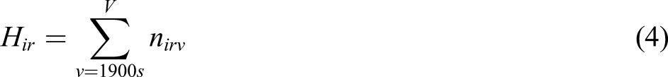
Equation (2) shows the urban ambience hedonic price model in the semi-log specification, indicating the proportion of houses in a specific cohort that are within walking distance from the transacted house. This study reports the results for both a 0.5 km (Model 2) and a 1.0 km radius (Model 3) walking distance.⁹ It measures both cohort clusters effect on urban ambience and the strength of the ambience effect. It does this by associating the proportion of houses of that cohort in two different sizes of the neighbourhood, with house density controlled

\ln (P_{i t s}) = α_{0} + α_{1} H_{i r} + \sum_{k = 1}^{K} γ_{k} X_{k i} + \sum_{v = 1910 s}^{V} δ_{v} N_{i r v} + \sum_{v = 1920}^{V} β_{v} C_{i v} + \sum_{t = 1}^{T} α_{t} D_{i t} + \sum_{s = 1}^{S} θ_{s} L_{i s} + ε_{i s t}

(2)

where H_ir denotes the total number of houses in the r-radius neighbourhood from the i^th house (Equation (4)) and α₁ measures the housing density effect; δ_v denotes the implicit price for the v^th cohort proportion in the r-radius neighbourhood N_irv (v = 1910s, 1920s, …, 2010s and r = 0.5 km and 1.0 km). N_irv is defined as in equation (3)

N_{i r v} = \frac{n_{i r v}}{H_{i r}}

(3)

H_{i r} = \sum_{v = 1900 s}^{V} n_{i r v}

(4)

where n_irv denotes the number of houses of cohort v in the r-radius neighbourhood from the i^th house.¹⁰

In this study, we use cohort rather than a functional form of age to proxy the ‘urban ambience’ effects. We do this because, on the one hand, the exact years since the completion of houses are not available; but on the other hand, the focus of this study is on the architectural styles of houses, which are evolving slowly over time. There were several significant shifts in architectural styles over the past century in New Zealand. The architectural styles of housing can be broadly characterised into five main categories based on their years of construction: the Victorian villa (the 1880s–1890s), the (California) Bungalow (1910s–1930s), the Art Deco (1930s–1940s), the State House (1940s–1960s) and the contemporary styled (1970s to now). The Victorian villa started to emerge circa the 1860s when Europeans began colonising the region. Entirely built with native timber, the villas were generally single-storey detached buildings in affluent suburbs. With decorated verandas, high ceilings, small windows, and wide hallways, they have been a part of New Zealanders’ lives for generations.

The Victorian villa is one of the most distinctive and predominant housing designs before World War I. The architectural style reveals that New Zealand architecture was heavily affected by the British Victorian period. During the Great Depression and inter-war period, influences from the United States were increasingly apparent. The bungalow first appeared in New Zealand around World War I and became the dominant style throughout the 1920s. Art Deco first appeared towards the end of the Great Depression in the early 1930s and lasted until after World War II. The style followed the trend from Europe after the great Exposition Internationale des Arts Décoratifs et Industriels Modernes held in Paris in 1925. The State House style resulted from a building programme to address the critical housing shortage in New Zealand by the Labour Government in the late 1930s. The majority of private houses built during this time also followed suit and looked very similar to those built under the government scheme. In the 1970s, New Zealand architecture underwent a major transition resulting in greater local individuality. Since then, there has been a variety of different housing styles, including ‘colonial’, ‘ranch’, ‘Mediterranean’, and ‘contemporary’. The 1990s brought a densification process involving increased numbers of townhouses and apartment buildings in the city centres. Era Design (2021) provides a detailed description of domestic architecture in New Zealand in various cohorts.

Data

The models are empirically tested using housing transaction data recorded by Auckland Central, New Zealand, from January 2010 to December 2019 (120 months). The dataset used in this study is from CoreLogic. To keep housing type and land tenure uniform, the study excludes apartment-type housing and leasehold interests from the transaction data. However, counting the number of houses in the neighbourhood takes apartment-type housing into account to test the ‘lack of atmosphere’ effect. The study also excludes all the transactions before January 2010, thereby minimising the change in urban ambiences due to redevelopments.

Further excluding some outliers, we identified 56,761 valid records. The data set also excludes the oldest two-decade cohorts, those built in the 1880s and 1890s, because the transactions of these cohorts are less than 0.15% of the total, and their price effects are found to be insignificant. Similarly, the counting of the number of houses in the neighbourhood also excludes these two cohorts. Supplemental Figure S1 in the supplementary material visualises the clusters of building cohorts in Auckland, New Zealand. The average nearest neighbour (ANN) distance statistics are used to give a first pass to test whether building cohorts have statistically significant clustering (Clark and Evans, 1954). The ANN test confirms that the cohort clusters reveal a spatial pattern that allows the urban ambience hypothesis to be further tested as a possible explanation of the cohort effect. For example, the houses built in the 1900s to the 1930s are highly concentrated in the Auckland central business district. Supplemental Figure S2 in the supplementary material shows a predominant form of pre-1920s residential architecture in Auckland. The dataset also provides a comprehensive list of variables on the characteristics of the property and neighbourhood. Supplemtnal Table S1 and Table S2 are placed in the appendices as supplementary materials to show the summary statistics of the cohort proportions in the neighbourhoods, and other variables.

Empirical results and robustness tests

Empirical results

Table 1 shows the results. Column (1) shows the baseline Model 1, which includes all the house transactions of the various cohorts. Almost all the variables are statistically significant at the 1% level, and the explanatory power of the model is reasonably high (the adjusted R-squared = 86.7%). The housing characteristics variables control the cohort effect, the view effect, the housing type effect and the size and facility effect. The cohort effects strongly confirm the impacts of the leaky homes crisis, as the coefficients for the 1990s and 2000s are the most negative. The effect is even more negative than that in the 1970s and the 1980s; that is, the cohort effects in the 1990s and 2000s properties are priced −12.8% and −9.5% less than new houses built in the 2010s (the omitted cohort variable), respectively, even though they are relatively new.

Table 1.

The results of Models 1, Model 2 and Model 3

	Model 1		Model 2 (r = 0.5km)		Model 3 (r = 1.0km)
Variables	Coefficient	t-stats	Coefficient	t-stats	Coefficient	t-stats
Constant	12.794^***	(133.31)	12.919^***	(128.48)	13.045^***	(127.80)
No_Bathrm	0.011^***	(5.18)	0.010^***	(4.97)	0.010^***	(4.70)
No_Bedrm	0.054^***	(24.28)	0.055^***	(24.56)	0.056^***	(25.09)
FLR_Area	0.002^***	(36.14)	0.002^***	(35.75)	0.002^***	(35.72)
IMPR_Value	2.98×10^−7***	(25.22)	2.96×10^−7***	(25.14)	2.97×10^−7***	(25.49)
Dist_CBD	−0.076^***	(−29.13)	−0.091^***	(−30.81)	−0.104^***	(−31.30)
CAT_D	−0.242^***	(−3.85)	−0.242^***	(−3.82)	−0.233^***	(−3.68)
CAT_F	−0.539^***	(−8.56)	−0.538^***	(−8.49)	−0.530^***	(−8.37)
CAT_M	0.068	(0.62)	0.067	(0.61)	0.092	(0.83)
C1900	0.205^***	(16.97)	0.204^***	(16.90)	0.204^***	(17.10)
C1910	0.234^***	(33.49)	0.225^***	(31.61)	0.228^***	(32.53)
C1920	0.182^***	(27.27)	0.168^***	(24.96)	0.170^***	(25.45)
C1930	0.156^***	(21.06)	0.144^***	(19.27)	0.144^***	(19.56)
C1940	0.114^***	(15.73)	0.111^***	(15.23)	0.105^***	(14.61)
C1950	0.087^***	(12.70)	0.082^***	(11.96)	0.083^***	(12.28)
C1960	0.021^***	(3.16)	0.015^**	(2.22)	0.015^**	(2.32)
C1970	−0.016^**	(−2.39)	−0.022^***	(−3.30)	−0.023^***	(−3.45)
C1980	−0.048^***	(−7.14)	−0.059^***	(−8.79)	−0.058^***	(−8.66)
C1990	−0.128^***	(−19.81)	−0.130^***	(−20.19)	−0.132^***	(−20.57)
C2000	−0.095^***	(−15.81)	−0.095^***	(−15.76)	−0.099^***	(−16.46)
H	—	—	−3.39×10^−5***	(−5.80)	−2.48×10^−5***	(−12.44)
N1900	—	—	−0.232^***	(−6.28)	−0.036	(−0.56)
N1910	—	—	0.339^***	(11.26)	0.195^***	(3.81)
N1920	—	—	0.355^***	(13.41)	0.689^***	(14.63)
N1930	—	—	0.151^***	(4.50)	−0.193^***	(−2.67)
N1940	—	—	−0.025	(−1.32)	0.068^**	(2.27)
N1950	—	—	0.077^***	(3.91)	0.012	(0.42)
N1960	—	—	0.071^***	(3.61)	0.201^***	(7.16)
N1970	—	—	0.053^***	(2.66)	−0.216^***	(−5.41)
N1980	—	—	0.375^***	(13.05)	0.970^***	(14.27)
N1990	—	—	−0.093^***	(−3.50)	−0.228^***	(−4.33)
NO VIEW	−0.066^***	(−7.47)	−0.061^***	(−6.97)	−0.061^***	(−6.91)
Slight View	−0.011	(−1.27)	−0.006	(−0.68)	−0.005	(−0.58)
Wide View	0.193^***	(14.41)	0.194^***	(14.60)	0.187^***	(14.10)
Centred VIF for Cyyyy variables	1.38–6.90		1.43–7.00		1.41–6.99
Centred VIF for Cyyyy variables	All coeff <10		All coeff < 10		All coeff < 10
Centred VIF for Nyyyy variables	NA		3.28–8.61		6.65–18.27
Centred VIF for Nyyyy variables			All coeff < 10		Two coeff > 10
Suburbs	Location fixed effect – See Supplemental Figure S3
Months	Time fixed effect – See Supplemental Figure S4
No. of Obs.	56,761		56,735		56,735
Adj.R-squared	0.867		0.869		0.870

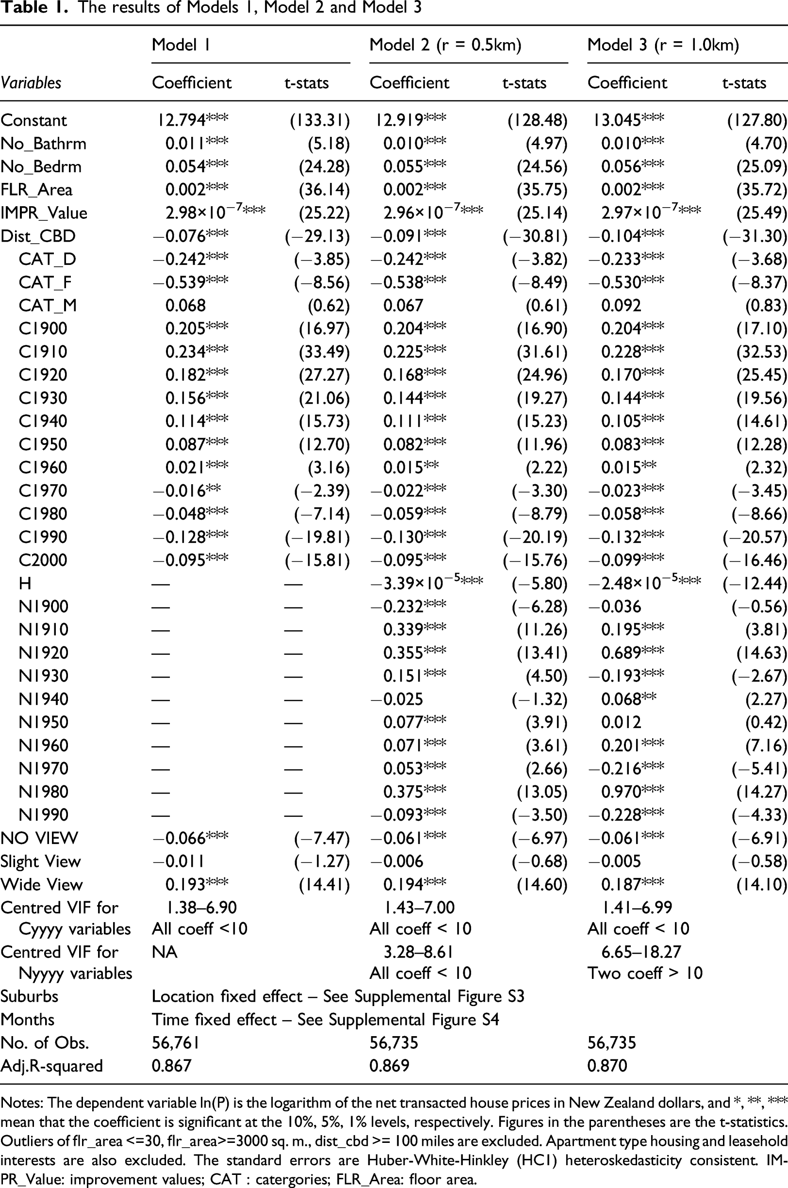
Notes: The dependent variable ln(P) is the logarithm of the net transacted house prices in New Zealand dollars, and *, **, *** mean that the coefficient is significant at the 10%, 5%, 1% levels, respectively. Figures in the parentheses are the t-statistics. Outliers of flr_area <=30, flr_area>=3000 sq. m., dist_cbd >= 100 miles are excluded. Apartment type housing and leasehold interests are also excluded. The standard errors are Huber-White-Hinkley (HC1) heteroskedasticity consistent. IMPR_Value: improvement values; CAT : catergories; FLR_Area: floor area.

In contrast, the oldest two cohorts (the 1910s and 1900s) are priced the highest, about 23.4% and 20.5% higher than the 2010s cohort. The positive and significant effect of improvement work, which is a valuer’s estimate of the depreciated construction cost of buildings on the site, also confirms that the depreciation effect (age effect) can be mitigated by renovation and rehabilitation. The negative signs of the housing type (CAT_D and CAT_F) effects reflect the price premium of vacant land (CAT_V, the omitted variable) over most of the other housing types. The view effects are also controlled reasonably by the valuers’ assessments of the views’ scopes. Houses with a wide (lack of) view command 19.3% more (−6.6% less) than houses with a modest view. Models 2 and 3 further control the density effect and the urban ambience effect. The leaky home cohorts are found to have about a 10% discount in their prices, which is close to the banks’ rule of thumb in mortgage loan assessments. The density effect is confirmed to be negative; that is, the higher the number of houses in the neighbourhood, the lower the house prices, yet the magnitude of the effect is relatively weak.

One focus of this study is on the cohorts’ neighbourhood effects, which are confirmed to be significant. Contrary to the linear depreciation assumption (i.e., age effect), this study finds that the historic cohorts (houses built in the 1910s and 1920s) enjoy a positive ambience effect. The top three most positive cohorts in their neighbourhood effects are those of the 1910s, 1920s and 1980s. The most significantly negative cohort in its neighbourhood effects is that of the 1990s, in the 0.5 km and 1.0 km radius neighbourhoods. However, the 1900s cohort imposes a negative and significant effect in a smaller 0.5 km radius neighbourhood, which may be explained by the development restrictions in preservation zones (Auckland Council, 2018) and will be examined in the robustness test. In other words, when the density effect, the house quality effect, and the view effect have been controlled, the house cohort is found to have an ambience effect (based on the proportion of the cohort cluster) on house prices.

Lastly, the time and location effects are controlled by the time and suburb dummies. The coefficients for suburbs and the house price indices of all the three models are shown in Supplemental Figure S3 and Figure S4 in the supplementary material. The suburb coefficients show that the location-fixed effects are substantially reduced because urban ambience effects explain part of the location effects due to house cohort clustering. The differences between the suburb coefficients in Models 1 and 3 (as shown by the shaded chart in Suplemental Figure S3) can be up to +0.189 on average. In contrast, the differences in month coefficients between Models 1 and 3 are only up to −0.002 on average.

Robustness tests

There are two major concerns in the above analysis. First, counting the cohort clusters is a snapshot at the end of 2019. The earlier transactions will have experienced more change in their counting due to redevelopments carried out in the period. Second, vintage effects are divided into two components: (1) the internal cohort effect related to the construction and workmanship of the transacted house itself; and (2) the ambience effect imposed by the cohort cluster in the neighbourhood. It is hard to disentangle the two when the cohort of transacted houses and the cohort of ambiences are similar. Therefore, we further conduct the following robustness test by re-estimating the models with recently built houses as a subsample (i.e. only including those completed in the 2000s and 2010s and transacted between 2002 and 2019) – Models 4 and 5. This minimises the temporal changes of the cohort clustering due to redevelopment and eliminates the internal cohort effects due to the nostalgic quality of old houses. It also excludes the effect of redevelopment restrictions on heritage houses in preservation zones.

Table 2 shows the results of the robustness test on the urban ambience effects by housing cohorts. The results for Models 4 and 5 are for the 0.5 km and 1.0 km radius neighbourhoods. They confirm the positive and significant price effect of the historic atmosphere, especially the ambiences of the 1910s and 1920s housing cohorts in the 0.5km distance model. But in the 1.0 km distance model they are statistically insignificant. This analysis also confirms both the adverse internal and external cohort effects of the 2000s cohort from potential leaky homes. The explanatory power of Models 4 and 5 is higher than that of Models 1 to 3, even though the number of variables is much smaller (fewer cohort variables).

Table 2.

The results of Models 4 and 5

Variables	Model 4 (r = 0.5km)		Model 5 (r = 1.0km)
	Coefficient	t-stats	Coefficient	t-stats
Constant	12.796^***	(61.48)	13.318***	(59.46)
No_Bathrm	0.009^**	(2.03)	0.009*	(1.91)
No_Bedrm	0.029^***	(3.60)	0.034***	(4.13)
FLR_Area	0.002^***	(8.01)	0.002***	(7.99)
IMPR_Value	2.71×10^−7***	(8.08)	2.70×10−7***	(7.96)
Dist_CBD	−0.068^***	(−7.47)	−0.082***	(−8.88)
CAT_F	−0.214^***	(−24.72)	−0.214***	(−24.00)
CAT_V	−0.119	(−1.56)	−0.124	(−1.65)
C2010	−0.101^***	(15.59)	−0.111***	(−17.67)
H	4.70×10^−5***	(3.15)	−2.57×10−5***	(−4.08)
N1900	0.187	(1.02)	0.144	(0.52)
N1910	0.229^*	(1.79)	−0.216	(−1.18)
N1920	0.173^**	(2.06)	0.142	(0.96)
N1930	−0.301^***	(−3.04)	−0.572**	(−2.52)
N1940	−0.085	(−1.55)	−0.088	(−1.01)
N1950	−0.025	(−0.53)	−0.247***	(−3.96)
N1960	−0.259^***	(−5.33)	−0.346***	(−4.17)
N1970	−0.058	(−0.99)	−0.048	(−0.40)
N1980	0.007	(0.14)	−0.103	(−1.05)
N1990	−0.320^***	(−4.40)	−0.747***	(−5.62)
N2000	−0.521^***	(−10.86)	−0.638***	(−7.08)
No View	−0.049^***	(−2.84)	−0.038**	(−2.14)
Slight View	−0.009	(−0.54)	0.001	(0.05)
Wide View	0.174^***	(6.88)	0.153***	(5.84)
Centred VIF for C2010 variables	3.12 < 10		2.81 < 10
Centred VIF for Nyyyy variables	3.29–13.07Two coeff > 10		4.58–26.28TEN coeff > 10
Suburbs	Location fixed effect – Yes
Months	Time fixed effect – Yes
No. of Obs	8,405		8,405
Adj.R-squared	0.886		0.885

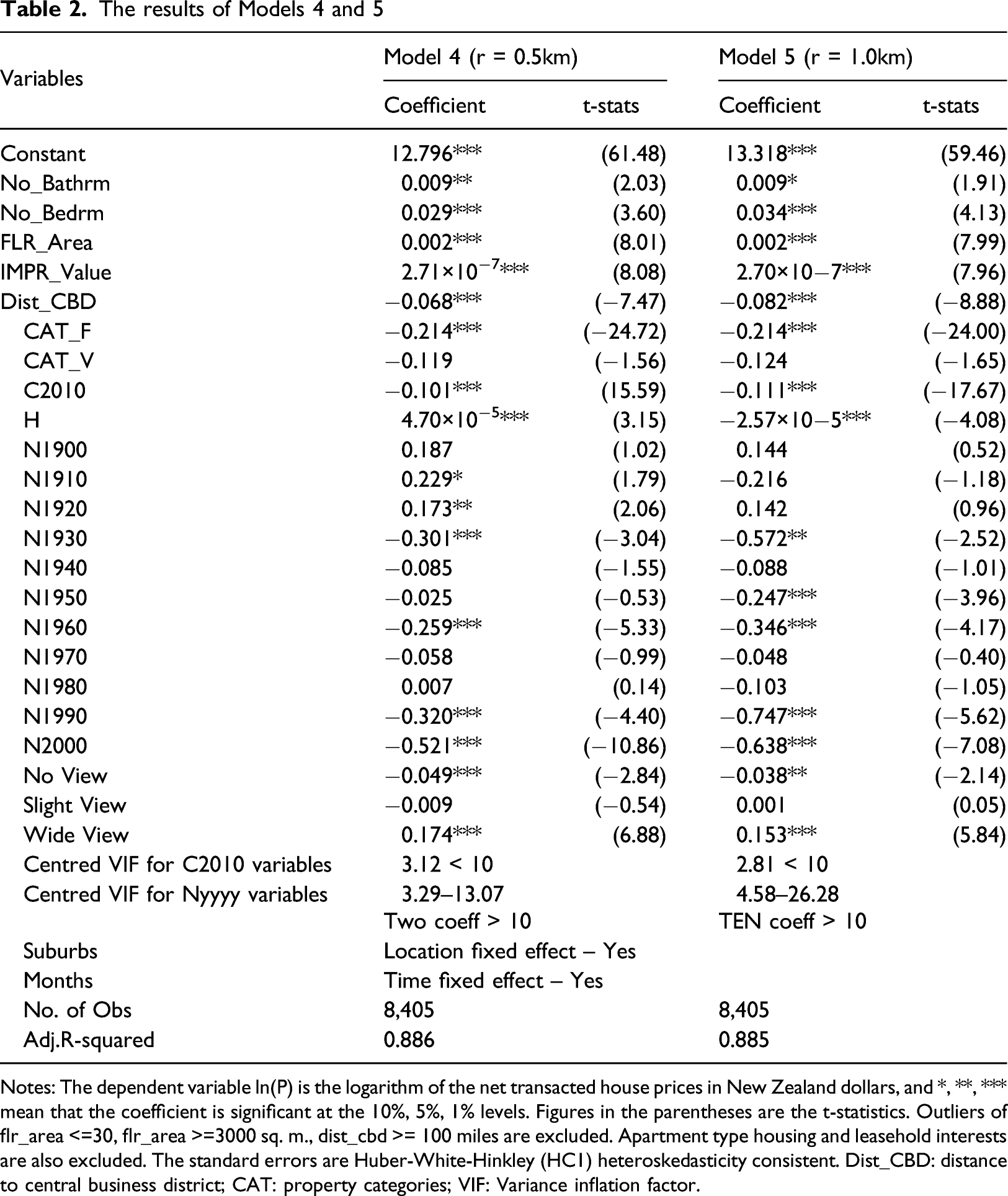
Notes: The dependent variable ln(P) is the logarithm of the net transacted house prices in New Zealand dollars, and ^*, ^**, ^*** mean that the coefficient is significant at the 10%, 5%, 1% levels. Figures in the parentheses are the t-statistics. Outliers of flr_area <=30, flr_area >=3000 sq. m., dist_cbd >= 100 miles are excluded. Apartment type housing and leasehold interests are also excluded. The standard errors are Huber-White-Hinkley (HC1) heteroskedasticity consistent. Dist_CBD: distance to central business district; CAT: property categories; VIF: Variance inflation factor.

Conclusions

The contribution of this paper is twofold. First, this is an initial attempt to disentangle the cohort effects in hedonic pricing analysis by providing non-linear external information, including the actual improvement values of the structures to indicate the depreciation/appreciation and the proportions of houses in each cohort in the neighbourhoods (cohort size). Second, this study is also novel in considering two separate forms of cohort effects, namely, the urban ambience effect (external effect) and the structural quality effect (internal effect) due to different house cohorts.

Methodologically, the estimated internal cohort effects are not merely a curve-fitting exercise but a hypothesis testing one using a-priori information on cohort workmanship. The magnitude of the leaky homes cohort (the 1990s and 2000s) discount (estimated to be about −10%) comes close to the banks’ assessments. More importantly, the tests identify a nostalgic value in old houses, especially those built in the 1910s and 1920s. The premium is more than 20% above the price of new houses. This result confirms the internal dimension of the cohort effect. Furthermore, the results show a positive and significant effect of the ‘historic atmosphere’ shaped by houses built in the 1910s and 1920s in both 0.5 km and 1.0 km radius neighbourhoods. The results confirm the external dimension of the cohort effects.

In addition, the neighbourhoods with leaky homes cohorts are also found to have a discount, implying that buyers discount neighbourhoods of the whole cohort even though the risk depends on the actual materials and design of the houses. However, it is worth noting that this study lacks micro-environment information that may have a confounding effect on house prices in the same neighbourhoods of the cohort clusters, although the chance of this effect is meagre given that 52 suburbs in the samples and two sizes of neighbourhoods are tested. The chance of confounding bias is relatively low. As such, we have conducted a robustness test by confining the transactions to only the cohorts built in the latest two decades to eliminate any heritage effects of the houses themselves. The results confirm both the internal and external cohort effects.

Unlike previous studies on urban ambiences, which have been studied in architecture and urban planning mostly by surveys and interviews of users, this study provides initial empirical evidence supporting the effect of urban ambiences created by different housing cohorts. It paves the way to further researching the market values of identified atmospheres, which may assist architects and planners in urban design. Urban aesthetics are known to be hard to quantify. An excellent urban aesthetic does not arise only from a cluster of architectural vintages (Burchard, 1957). This initial attempt to quantify urban aesthetics by measuring the clusters of housing cohorts will open a new door for exploring the urban aesthetic.

Traditionally, urban planners have tried to designate land uses to mitigate zoning mismatch (Talen et al., 2016). With rising public concerns for heritage preservation and tourism, more planners and scholars of urban studies have started investigating ‘harmonic planning’ for preserving or shaping the urban landscape. Harmonic planning in architecture is an exploration of possible intersections between architecture and interaction design that mitigates the mismatch in ambience. For example, Zagroba et al. (2020) found that the harmonious planning of public spaces influences perceptions of space considerably. Heide et al. (2007) studied the importance of ambience on tourism and hospitality. This study also confirms the positive effect of clusters of uniform architectural ambience on house prices in the vicinity. The results of this study can be used to assess the value of architectural order, which is a cost-benefit analysis that may be a crucial component for urban design and revitalisation programmes. The present findings also constitute valuable inputs for urban planners and designers who wish to consider imposing measures to protect the harmonic clustering of architectural ambience. This study always reminds us that architecture is not all about the design of the building; it is also about the cultural setting and the ambience: it is the integrated whole that matters.

Supplemental Material

sj-pdf-1-epb-10.1177_23998083211064625 – Supplemental Material for The economics of architectural aesthetics: Identifying price effect of urban ambiences by different house cohorts

Supplemental Material, sj-pdf-1-epb-10.1177_23998083211064625 for The economics of architectural aesthetics: Identifying price effect of urban ambiences by different house cohorts by Ka Shing Cheung and Chung Yim Yiu in Environment and Planning B: Urban Analytics and City Science

Footnotes

Acknowledgements

We would like to express our great appreciation to Dr. Jiamou Liu and Dr. Kaiqi Zhao from the School of Computer Science for their generous and constructive advice in discussing and designing the spatial counting program. Our gratitude is also extended to Mr Jian Cheng for his excellent support in writing the python program code for spatial counting. We would also like to thank Ms Eileen Li from COMPASS for her technical support in executing the spatial counting program in the New Zealand eScience Infrastructure (NeSI). Special thanks should be given to the Centre for e-Research to connect us to the national high-performance computing platform NeSI. We would also like to extend my thanks to Emeritus Professor Kerr Inkson for sharing his advice during the course of this research. We are also immensely grateful to anonymous reviewers for their comments on an earlier version of the manuscript. Any errors are our own and should not tarnish the reputations of these esteemed persons.

Declaration of conflicting interests

The author(s) declared no potential conflicts of interest with respect to the research, authorship, and/or publication of this article.

Funding

The author(s) disclosed receipt of the following financial support for the research, authorship, and/or publication of this article: This research is financially supported by the University of Auckland Faculty Research Development Fund.

ORCID id

Ka Shing Cheung

Supplemental material

Supplemental material for this article is available online.

Notes

Author Biographies

Dr. Ka Shing Cheung is a Senior Lecturer in the Department of Property at the University of Auckland Business School. His research focuses on understanding the role of government as an institution in shaping the urban real estate market. He was a recipient of the Fulbright Research Scholar Award and affiliated at the University of California, Los Angeles, and also the Australian Endeavour Research Fellow at The University of Melbourne in recognition of his research excellence in affordable housing and urban studies research.

Dr. Chung Yim Yiu is an Associate Professor in the Department of Property at the University of Auckland. He is currently one of the Faculty Research Committee members. He has written and researched widely on housing policy and housing price analysis. He has also linked his research to practice; he was the elected candidate representing the Architectural, Surveying, Planning and Landscape Functional Constituency in the Legislative Council of Hong Kong in 2016 and a Fellow of the Royal Institution of Chartered Surveyors.

References

Abusaada

Elshater

(2020) Effects of Urban atmospheres on changing attitudes of crowded public places: an action plan. International Journal of Community Well-Being 3: 109–159.

Abusaada

Salama

Elshater

(2020) Reconstructing Urban Ambience in Smart Public Places. Hershey: Engineering Science Reference

Ahlfeldt

Mastro

(2012) Valuing iconic design: frank lloyd wright architecture in oak park, Illinois. Housing Studies 27(8): 1079–1099.

Ahlfeldt

Maennig

(2010) Substitutability and complementarity of urban amenities: external effects of built heritage in Berlin. Real Estate Economics 38(2): 285–323.

Anselin

Bera

(1998) Spatial dependence in linear regression models with an introduction to spatial econometrics. In: Ullah

Giles

(eds) Handbook of Applied Economic Statistics. New York, NY: Marcel Dekker, 237–289.

Anselin

Lozano-Gracia

(2009) Spatial hedonic models. In Palgrave Handbook of Econometrics. London, UK: Palgrave Macmillan, 1213–1250.

Auckland Council (2018) Auckland’s Heritage Counts 2018 – Annual Summary. Auckland, New Zealand: Auckland Council. https://www.aucklandcouncil.govt.nz/arts-culture-heritage/heritage/docsheritagecountssummaries/aucklands-heritage-counts-2018.pdf

Bade

Castillo

Fernandez

Aguilar-Bohorquez

(2020) The price premium of heritage in the housing market: evidence from Auckland, New Zealand. Land Use Policy 99: 105042.

Basu

Thibodeau

(1998) Analysis of spatial autocorrelation in house prices. The Journal of Real Estate Finance and Economics 17(1): 61–85.

10.

Böhme

(2017). Atmospheric architectures: The aesthetics of felt spaces. In: Engels-Schwarzpaul

Trans (ed). London, UK: Bloomsbury Academic.

11.

Borch

(2014) Architectural atmospheres: On the Experience and Politics of Architecture. Basel, Switzerland: Birkhauser, 18–41.

12.

Buitelaar

Schilder

(2017) The economics of style: measuring the price effect of neo‐Traditional architecture in housing. Real Estate Economics 45(1): 7–27.

13.

Burchard

(1957) The urban aesthetic. The ANNALS of the American Academy of Political and Social Science 314(1): 112–122.

14.

Cartern

Haloupek

(2000) Spatial autocorrelation in a retail context. International Real Estate Review 3(1): 34–48.

15.

Chau

Wong

Yiu

(2003) Price discovery function of forward contracts in the real estate market: an empirical test. Journal of Financial Management of Property and Construction 8(3): 129–137.

16.

Clark

Evans

(1954) Distance to nearest neighbor as a measure of spatial relationships in populations. Ecology 35: 23–30.

17.

Coulson

Lahr

(2005) Gracing the land of elvis and beale street: historic designation and property values in memphis. Real Estate Economics 33(3): 487–507.

18.

Coulson

Leichenko

(2001) The internal and external impact of historical designation on property values. The Journal of Real Estate Finance and Economics 23(1): 113–124. DOI: 10.1023/A:1011120908836.

19.

Coulson

McMillen

(2008) Estimating time, age and vintage effects in housing prices. Journal of Housing Economics 17(2): 138–151. DOI: 10.1016/j.jhe.2008.03.002.

20.

Era Design (2021) Architectural Eras. (accessed 17 January 2022). Available at: https://www.eradesign.co.nz/wp-content/uploads/2016/06/Architectural-Eras.pdf.

21.

Elgin

(2010) The Impact of Neighbourhood Characteristics and Support on Well-Being, Housing Satisfaction, And Residential Stability for People With Mental Illness. Christchurch, New Zealand: Master`s thesis, University of Canterbury.

22.

Fernandez

Bucaram

(2019) The changing face of environmental amenities: heterogeneity across housing submarkets and time. Land Use Policy 83: 449–460.

23.

Foltête

Piombini

(2010) Deviations in pedestrian itineraries in urban areas: a method to assess the role of environmental factors. Environment and Planning B: Planning and Design 37(4): 723–739.

24.

Francke

Minne

AMV

(2017) Land, structure and depreciation. Real Estate Economics 45(2): 415–451.

25.

Franco

Macdonald

(2018) The effects of cultural heritage on residential property values: evidence from Lisbon, Portugal. Regional Science and Urban Economics 70: 35–56.

26.

Gandy

(2017) Urban atmospheres. Cultural Geographies 24(3): 353–374.

27.

Gillen

Thibodeau

Wachter

(2001) Anisotropic autocorrelation in house prices. Journal of Real Estate Finance and Economics 23(1): 5–30.

28.

Glaeser

Kincaid

Naik

(2018) Computer Vision and Real Estate: Do Looks Matter and Do Incentives Determine Looks. NBER Working Paper 25174 http://www.nber.org/papers/w25174.pdf.

29.

Goodman

Thibodeau

(1995) Age-related heteroskedasticity in hedonic house price equations. Journal of Housing Research 6(1): 25–42. Available at: http://www.jstor.org/stable/24825889.

30.

Griffith

(1992) What is spatial autocorrelation? Reflections On The Past 25 Years Of Spatial Statistics. Paris: L’Espace Géographique, 265–280.

31.

Hamid

(2001) Incorporating A Geographic Information System in Hedonic Modelling of Farm Property Values. PhD eds. Lincoln, UK: Lincoln University.

32.

Harkness

Newman

Salkever

(2004) The cost-effectiveness of independent housing for the chronically mentally ill: do housing and neighbourhood features matter? Health Services Research 39(5): 1341–1360.

33.

Heide

Lærdal

Grønhaug

(2007) The design and management of ambience – Implications for hotel architecture and service. Tourism Management 28(5): 1315–1325.

34.

Hencher

Tyson

Hutchinson

(2005) Investigating substandard piles in Hong Kong. In: Neale

(ed) Forensic Engineering: The Investigation of Failures. London, UK: Institute of Civil Engineers.

35.

Heppel

(2000) Spatial autocorrelation. In: Johnston

Gregory

Pratt

Watts

(eds) The Dictionary of Human Geography. 4th edition. Oxford, UK: Blackwell Publishers.

36.

Kim

J-H

Kil

Park

(2018) The influence of urban landscape spatial patterns on single-family housing prices. Environment and Planning B: Planning and Design 45(1): 26–43.

37.

Lazrak

Nijkamp

Rietveld

Rouwendal

(2014) The market value of cultural heritage in urban areas: an application of spatial hedonic pricing. Journal of Geographic Systems 16(1): 89–114.

38.

Leichenko

Coulson

Listokin

(2001) Historic preservation and residential property values: an analysis of Texas cities. Urban Studies 38(11): 1973–1987.

39.

Lindenthal

Johnson

(2018) Machine Learning, Building Vintage and Property Values Working Paper. Cambridge, UK: Cambridge Real Estate Machine Learning Lab.

40.

Mares

Desai

Rosenheck

(2005) Association between community and client characteristics and subjective measures of the quality of housing. Psychiatric Services 56(3): 315–319.

41.

Moro

Mayor

Lyons

Tol

RSJ

(2013) Does the housing market reflect cultural heritage? A case study of greater dublin. Environment and Planning A 45(12): 2884–2903.

42.

Naik

Raskar

Hidalgo

(2016) Cities are physical too: using computer vision to measure the quality and impact of urban appearance. American Economic Review 106(5): 128–132.

43.

Noonan

(2007) Finding an impact of preservation policies: price effects of historic landmarks on attached homes in Chicago, 1990–1999. Economic Development Quarterly 21(1): 17–33.

44.

Norberg-Schulz

(1980) Genius Loci: Towards a Phenomenology Of Architecture. London, UK: Academy Editions.

45.

Nunns

Hitchins

(2015) The Value Of Land, Floorspace, And Amenities: A Hedonic Price Analysis Of Property Sales In Auckland 2011-2014. Auckland Council. https://knowledgeauckland.org.nz/media/1321/tr2015-012-value-of-land-floorspace-and-amenities-auckland.pdf (Retrieved on 7 Aug 2020).

46.

O’Brien

(2011) The age–period–cohort conundrum as two fundamental problems. Quality & Quantity 45(6): 1429–1444.

47.

O’Brien

Stockard

Isaacson

(1999) The enduring effects of cohort characteristics on age-specific homicide rates, 1960-1995. American Journal of Sociology 104: 1061–1095.

48.

PfliegerPattaroni

Jemelin

Kaufmann

(2008) The Social Fabric of the Networked City. Oxford, UK: Routledge.

49.

PricewaterhouseCoopers (2009) Weathertightness – Estimating the Cost, for the Department of Building and Housing . London, UK: PricewaterhouseCoopers (PwC). https://www.interest.co.nz/sites/default/files/PWC-leakyhomesreport.pdf

50.

Randolph

(1988) Housing depreciation and aging bias in the consumer price index. Journal of Business and Economic Statistics 6(3): 359–371.

51.

Rehm

Cheung

Filippova

Patel

(2019) Stigma, risk perception and the remediation of leaky homes in New Zealand. New Zealand Economic Papers 54(1): 89–105.

52.

Sirmans

Macdonald

Macpherson

Zietz

(2006) The value of housing characteristics: a meta-analysis. The Journal of Real Estate Finance and Economics 33(3): 215–240.

53.

Stefansdottir

(2018) The role of urban atmosphere for non-work activity locations. Journal of Urban Design 23(3): 319–335.

54.

Talen

Anselin

Lee

Koschinsky

(2016) Looking for logic: The zoning-land use mismatch. Landscape and Urban Planning 152: 27–38.

55.

Thibaud

J-P

(2015) The backstage of urban ambiences: when atmospheres pervade everyday experience. Emotions, Space and Society 15: 39–46.

56.

S-M

Sun

(2004) Transaction-based office price indexes: a spatiotemporal modeling approach. Real Estate Economics 32(2): 297–328.

57.

Wigley

(1998) Architecture of atmosphere. Daidalos 68: 18–27.

58.

Williams

(1954) Urban aesthetics: an approach to the study of the aesthetic characteristics of cities. The Town Planning Review 25(2): 95–113.

59.

Zagroba

Szczepańska

Senetra

(2020) Analysis and evaluation of historical public spaces in small towns in the polish region of warmia. Sustainability 12: 8356.

60.

Zumthor

(2006) Atmospheres: Architectural Environments - Surrounding Objects. Basel, Switzerland: Birkhauser. (accessed on Mar 8 2021).

Supplementary Material

Please find the following supplemental material available below.

For Open Access articles published under a Creative Commons License, all supplemental material carries the same license as the article it is associated with.

For non-Open Access articles published, all supplemental material carries a non-exclusive license, and permission requests for re-use of supplemental material or any part of supplemental material shall be sent directly to the copyright owner as specified in the copyright notice associated with the article.

0.00 MB

0.56 MB