Sage Journals: Discover world-class research

Abstract

Cities in developing countries share a pattern of accelerated and largely unplanned urbanization that results in internal socioeconomic inequalities. The modeling of urban growth with spatial distribution of socioeconomic groups has been studied only to a limited extent. This paper proposes a method to simulate both urban growth and the socioeconomic group that is likely to settle in a particular location as a function of local environmental characteristics. Using a cellular automata model, newly urbanized cells are identified and then, as a post-processing step, distributed among five socioeconomic groups in a preferential settlement selection process. A land value map learned with a random forest regressor is used for this purpose. Our case study is Greater Mexico City during the period 1997–2010. We identified that the main features influencing the location of socioeconomic groups are the closest socioeconomic group, the distance to water bodies, and the distance to the urban center. This suggests that the newly urbanized cells are likely to settle in neighborhoods of similar socioeconomic levels. Moreover, the increasing distance from the urban center results in a generally decreasing land value. However, regions with a high land value were also found in remote areas where environmental features that improve the ecosystem services are present.

Keywords

Urbanization cellular automata land value map random forest regression Greater Mexico City

Introduction

The share of global population living in urban areas is steadily increasing (UN Department of Economic and Social Affairs, 2018). In recent decades, the majority of this increase has occurred in developing countries, where cities share a pattern of accelerated and largely unplanned urbanization (Duque et al., 2019; García-Ayllón 2016; Leao et al., 2004). The rapid growth of cities has, in many cases, outpaced the capacity of local authorities to meet the demand of housing and urban services of the growing population (García-Ayllón 2016; Jaitman 2015). This has resulted in serious problems such as low quality public services with limited coverage, social inequality, high levels of pollution, and the degradation of the local environment (Bonilla-Bedoya et al., 2020; García-Ayllón 2016; Guzman et al., 2020; Wu et al., 2010).

The impacts of urbanization are not distributed homogeneously within urban areas. Consequently, they contribute to internal socioeconomic inequalities which are often translated as spatial segregation (Azhdari et al., 2018; Vermeiren et al., 2016). This unevenness in the distribution of social groups across the physical space of the city (White 1983; Reardon and O’Sullivan 2004) is caused by complex interactions between different social groups whose preferences are constrained by external factors including political strategies and economic development at the macro-scale. However, even with such constraints, where people settle within the city is usually a matter of lifestyle and, more importantly, income. High-income individuals can choose the location of their housing, usually on high-value land, whereas low-income residents often end up in sites of lesser land value and, in some cases, are even forced to occupy land informally (Azhdari et al., 2018; Barros 2004; Frenkel and Israel 2018; Vermeiren et al., 2016). The resulting urban form not only influences the city’s economic performance and quality of life but also the local use of resources and its environmental impact (Duque et al., 2019; Lyu et al., 2019).

Despite the fact that urban growth and the resulting social structure go hand in hand, there is a lack of simple and transparent tools that simulate the dynamics of urbanization and the arising spatial distribution of socioeconomic groups. To close this gap, this paper proposes a method to simulate urban growth and the socioeconomic group that is likely to settle in a particular location as a function of local environmental characteristics. To this end, we extend an adapted version of a well-known cellular automata urban growth model by adding a machine-learned land value layer to spatially distribute new urban cells according to their socioeconomic status as a post-processing step. This work intends to serve as a tool to support the development of urban policies for growing cities, especially in developing countries.

Literature review

Different urban growth models for understanding and modeling urban growth processes have been developed and reviewed in the last decades (Aburas et al., 2016; Agarwal et al., 2002; Batty 2012; Gounaridis et al., 2019; Vermeiren et al., 2016). Cellular automata (CA) models have shown potential in representing and simulating the complexity of the urbanization process (Aburas et al., 2016; Batty and Longley 1994; Berberoğlu et al., 2016; Dietzel and Clarke 2007). CA is a bottom-up modeling approach that captures the dynamics of urban growth with simple local rules that influence the state of discrete cells in discrete urban growth cycles. Its main advantages are its simplicity, transparency and powerful capabilities, and particularly, its full consistency with Geographic Information Systems (GIS) (Aburas et al., 2016; Clarke et al., 1997; Gounaridis et al., 2019; Leao et al., 2004; Mustafa et al., 2018; Wu et al., 2010). Moreover, the high flexibility of CA models allows the loose or hard coupling of other models to enhance the simulation capabilities for specific applications (Aburas et al., 2016). These include, for example, the integration of machine-learning techniques for learning transition rules (Almeida et al., 2008; Gounaridis et al., 2019; Li and Yeh 2002; Mustafa et al., 2018) and the coupling of other models such as Markov chains (Kamusoko et al., 2009), socioeconomic models (Wu et al., 2010), and environmental impact models (Lyu et al., 2019; Paiva et al., 2020). Furthermore, it is possible to remove the limitation of discrete states in CA models by applying fuzzy logic (Liu 2010; Ntinas et al., 2017).

Demographic and economic factors at the macro-scale are important determinants of urbanization (Gu 2019; Jedwab et al., 2017) and also have an impact on the structure and morphology of the city (Azhdari et al., 2018). However, as a bottom-up approach, CA models cannot explicitly model these driving forces. This problem is partially solved by the inclusion of an exogenous urban land demand that determines the path of urbanization (Houet et al., 2016; Wu et al., 2010). Most CA models use historic urbanization maps to determine such path in the form of urban growth coefficients (Batty and Longley 1994), probability maps (Rienow and Goetzke 2015), or complex transition rules (Gounaridis et al., 2019; Mustafa et al., 2018). Nevertheless, these approaches do not consider the relationship between spatial driving forces and intra-urban dynamics, and consequently, overlook the resulting spatial segmentation of different social groups.

On the other hand, several studies have analyzed the spatial segmentation arising from urbanization but without a link to urban growth models (Jean et al., 2016; Wurm et al., 2019; Zhao et al., 2019). Few studies cover both the analysis and/or simulation of the urbanization process and the resulting social structure. Mustafa et al. (2018) simulates the intra-urban structure originated from urban growth by integrating a multinomial logistic regression and CA to examine the built-up development with different urban densities. A socioeconomic indicator, richness index, is identified as one of the main causative factors for determining the built-up density. Thus, this approach enables an indirect simulation of the distribution of social groups. Azhdari et al. (2018) use a logistic regression model to calculate the local effect of the driving forces of urban growth and explore their relationship to socioeconomic segregation in Shiraz, Iran. They found that while affluent residents could choose to live near large urban centers or in remote locations but with far superior environmental conditions, the poorer strata could not live near large economic centers and were pushed into areas unsuitable for living. Barros (2004) and Vermeiren et al. (2016) propose agent-based models to simulate both urban expansion and social dynamics of a developing city. Both define location selection and displacement functions for each agent (household) belonging to a socioeconomic group. Agents first settle at grid cells with the highest utility value and then interact according to their predefined functions resulting in high-income groups settling in high-value land and low-income groups being displaced to lower-value areas. In a similar way, Santos et al. (2014) propose a grid-based agent-based model where agents move according to their accessibility preferences within newly urbanized cells.

Though suitable for the simulation of the intra-urban dynamics, functions of agent-based models are usually less transparent to articulate the relationship between local environment variables and urban growth than CA transition rules (Santos et al., 2014). Therefore, in this work, we combine the simplicity and transparency of CA models to simulate urban growth and then, as a post-processing step, we simulate the intra-urban dynamics. These are modeled as a preferential settlement selection based on the expected fraction of cells of specific socioeconomic groups and a land value map. Cells with higher land values accommodate social groups with higher socioeconomic status, while groups with lower socioeconomic status end up occupying land of lower value.

Methodology

A high level workflow of the proposed urban growth model is presented in Figure 1. Our approach consists of three main processes. In the first process, P1, the georeferenced input data, consisting of gridded layers of historic socioeconomic data and environmental characteristics in a high spatial resolution are used to learn the value of urbanized land. We follow a supervised learning approach in which a random forest regressor (RFR) is trained with the socioeconomic status of settlements as labels together with the environmental characteristics as features. The output of P1 is a land value map. In the second process, P2, a subset of the environmental features along with a supplementary urban seed layer are input to the CA urban growth model. An adapted version of the popular SLEUTH model was developed in Python for this purpose to have a seamless integration of the processes P1 and P2 in one simulation tool. In the third process, P3, the newly urbanized cells from the simulated urban growth in P2 are allocated to a predefined distribution of socioeconomic groups according to the land value map from P1. This is done for every growth cycle. As a result, the extended CA model associates a socioeconomic level to every new urban cell in the study area. The final outcome is a set of maps depicting urban growth stratified by socioeconomic level. The Python scripts developed for the three processes are available online at Molar-Cruz and Pöhler, 2020.

Figure 1.

General workflow for the simulation of urban growth disaggregated by socioeconomic groups.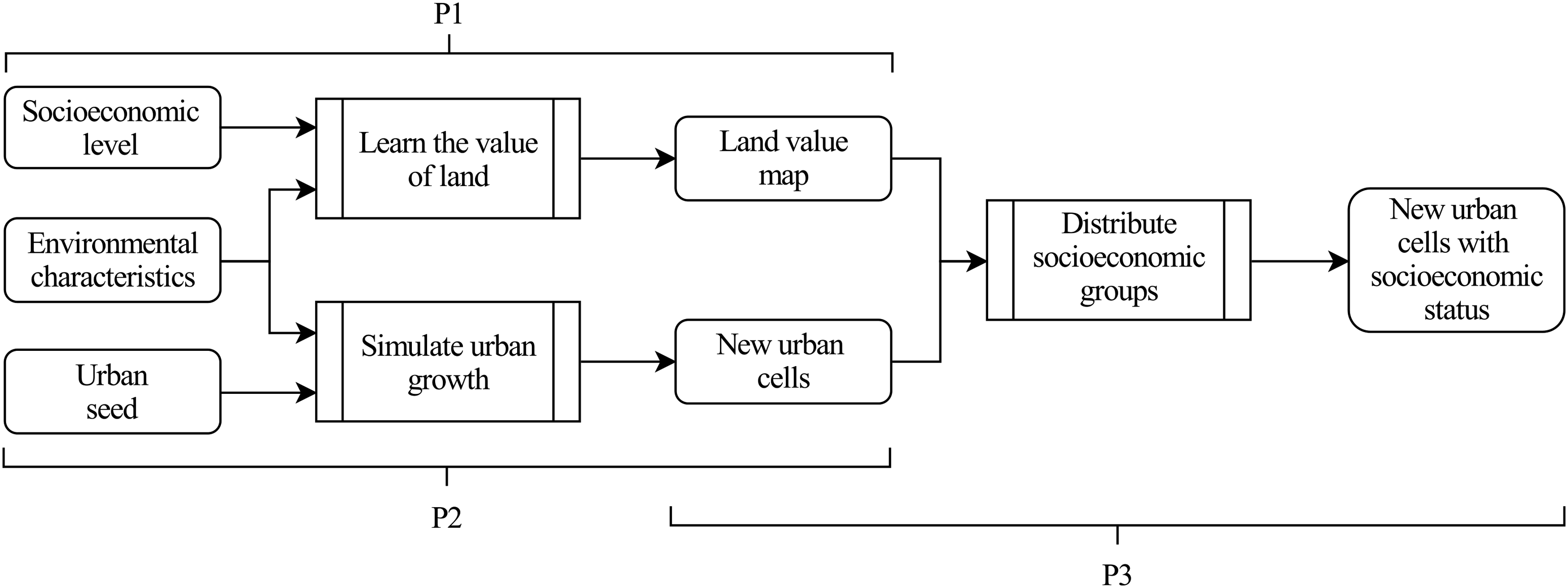

P1: Learning the value of land

The location of a cell with respect to social and environmental amenities can be used as a proxy to calculate the value of land. In order to learn the value of land, each label, that is, the socioeconomic level of an urban cell, together with its features, that is, the environmental characteristics at the cell location are used to train an RFR. The trained RFR is applied to predict the socioeconomic group likely to settle at a specific location depending on the environmental characteristics. Using this predictions, we generate a land value map. A short explanation on RFR, a schematic representation of the method (Supplemental Figure S1), as well as references for further details on this data-driven approach are found in the Supplementary Material.

P2: Simulating urban growth

We simulate urban growth using a Python-based CA model built on the four urban growth rules of the widely-used SLEUTH model (Clarke et al., 1997) with minor modifications. These concern the definition of global probabilities of urbanization and the calibration of urban growth coefficients. The urban growth model is available online at (Molar-Cruz and Pöhler, 2020).

Starting with a grid of binary cells representing urban and non-urban areas at a specific time, newly urbanized cells are determined in each growth cycle by four transition rules: spontaneous growth, new spreading center growth, edge growth and road-influenced growth. These are applied to all cells within the study area and depend on the environmental features of the neighborhood including slope, excluded areas, urban regions and transportation infrastructure.

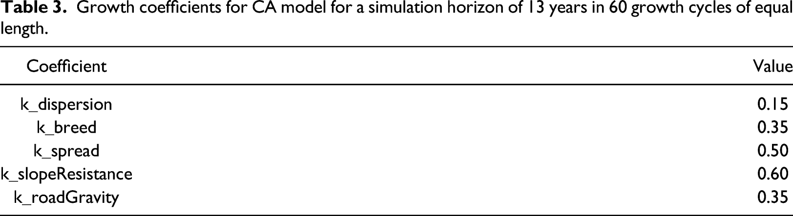
Spontaneous growth represents random settlement on non-urban land. New spreading center growth deals with the generation of new urban centers from the previous spontaneously grown cells. Edge growth simulates the natural outward spread of a city at its edges. All neighborhoods with at least three urbanized cells are subject to edge growth. Road-influenced growth accounts for the effect of transportation networks in the urbanization process facilitating settlements if found within the neighborhood. Five coefficients control the behavior of the CA by influencing the local probability of urbanization in the four growth rules: k_dispersion defines how dispersed the growth happens, k_breed determines how likely a new settlement initiates surrounding growth as a spreading center, k_spread influences the amount of natural growth of the city at its edges, k_slopeResistance refers to the weight of the slope in reducing the likelihood of a cell to be urbanized, and k_roadGravity influences how strongly the settlements are attracted by roads. Different to Clarke’s model, we consider that the global probability for spontaneous urban settlement decreases linearly with increasing distance from the urban seed. Further details on the growth rules with graphical examples are given in Supplemental Figure S2 in the Supplementary Material.

P3: Distributing socioeconomic groups

For each growth cycle, and after the execution of the growth rules for the entire grid, the land values of the newly urbanized cells are retrieved and sorted in descending order. Depending on their rank, cells are distributed among five socioeconomic groups simulating a preferential settlement selection. As a result, the highest socioeconomic group occupies all cells with the highest land value until the expected number of cells of this group is reached. This is followed by the second highest socioeconomic group and so on until all new cells, that is, the newly urbanized land, are distributed among the socioeconomic groups. The expected fraction of urban extent per socioeconomic group is determined exogenously based on the historic population size and spatial distribution of socioeconomic groups within the study area. Therefore, this approach does not directly incorporate external factors, such as economic growth, or internal factors, such as recontextualization of city quarters, that might affect the size of each socioeconomic group and the area they occupy within the city.

Data

Our study case is Greater Mexico City, one of the biggest metropolitan areas in the world with a population of 21.58 million inhabitants in 2018 (UN Population Division 2018). We analyze the urban expansion and intra-urban dynamics between 2000 and 2010. The input data used to carry out our approach is summarized in Table 1. The process in which each raw dataset was used is also presented in this table. Many of the raw datasets were not used directly. Instead, they are transformed into distances which are more suitable indicators. Such datasets are marked with a (*) and are described in the following subsections. The available datasets differ in source years. However, most of them are within the 2000–2010 period. We assume that the environmental characteristics from layers outside this time frame do not differ significantly from those of this period.

Table 1.

Name, description, year, and source of raw input datasets. The process in which the dataset is used is in the column “Process”. Starred (*) datasets are preprocessed.

Name	Description	Year	Source	Process
IMU*	Urban marginalization index	2000, 2005, 2010	CONAPO (2010)	P1
Droughts	Degree of drought risk	2012	CENAPRED (2012a)	P1
Floods	Degree of flood risk	2007	CENAPRED (2007)	P1
Climatology	10-year land cover	2001–2010	Broxton et al. (2014)	P1
Soil degradation	Type of soil degradation	2004	SEMARNAT-CP (2004)	P1
Toxicity	Toxicity hazard	2012	CENAPRED (2012b)	P1
Wells*	Water supply wells	2015	INEGI (2015)	P1
Wastewater*	Wastewater treatment plants	2015	INEGI (2015)	P1
DEM*	Digital elevation model	2000	NASA JPL (2013)	P1/P2
Land use*	Urban areas and water bodies	1997	INE (1997)	P1/P2
Protected areas	Federal, state and municipal protected areas	2015, 2017	CONABIO (2015); CONANP (2017)	P1/P2
Roads*	Highway network	1985	Dig Chart of the World (1985)	P1/P2

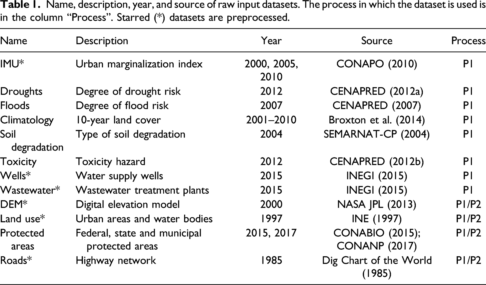
The resolution of the datasets varies from regular 30 m by 30 m cells to irregular shapes of several thousand square meters in the case of the IMU dataset. In the latter, the marginalization index is given for each urban basic geographic unit (AGEB), whose surface area varies in size. All input geodatasets are rasterized into a grid with a spatial resolution of 90 m by 90 m. This resolution allows both a meaningful interpretation of urbanized cells and a practical aggregation of the input data with the highest granularity. This results in a grid of 14 250 km² distributed in 1.76 million cells.

Input data for P1

Socioeconomic level as label

We use the inverse of the urban marginalization index (IMU) as the socioeconomic level. The IMU was published by the Mexican National Population Council (CONAPO) for the years 2000, 2005, and 2010. It measures the social deprivation of the urban population at the AGEB level considering different dimensions such as health, education, living conditions and property (CONAPO 2010). This dataset categorizes urban marginalization in five levels which are translated into five socioeconomic groups. These are sorted from one to five, with group 1 being the AGEBs with the highest land value or lowest social deprivation, and group 5 those with the lowest land value or highest social deprivation. Additional details on the IMU, including the number of samples and basic statistics (Supplemental Table S1) and the ranges of marginalization index for the definition of the five groups (Supplemental Table S2), are available in the Supplementary Material. Figure 2 shows the spatial distribution and the fraction of urban extent by socioeconomic group of the newly urbanized cells during the period 1997–2010. The distribution of socioeconomic groups within the urban seed is visualized in Supplemental Figure S3.

Figure 2.

Spatial distribution of socioeconomic groups of urbanized cells in Greater Mexico City during the period 1997–2010. The urban seed, which corresponds to the existing urban area in 1997, is displayed in black. The AGEBs within this area are not considered for the calculation of the fraction of urban extent by socioeconomic group.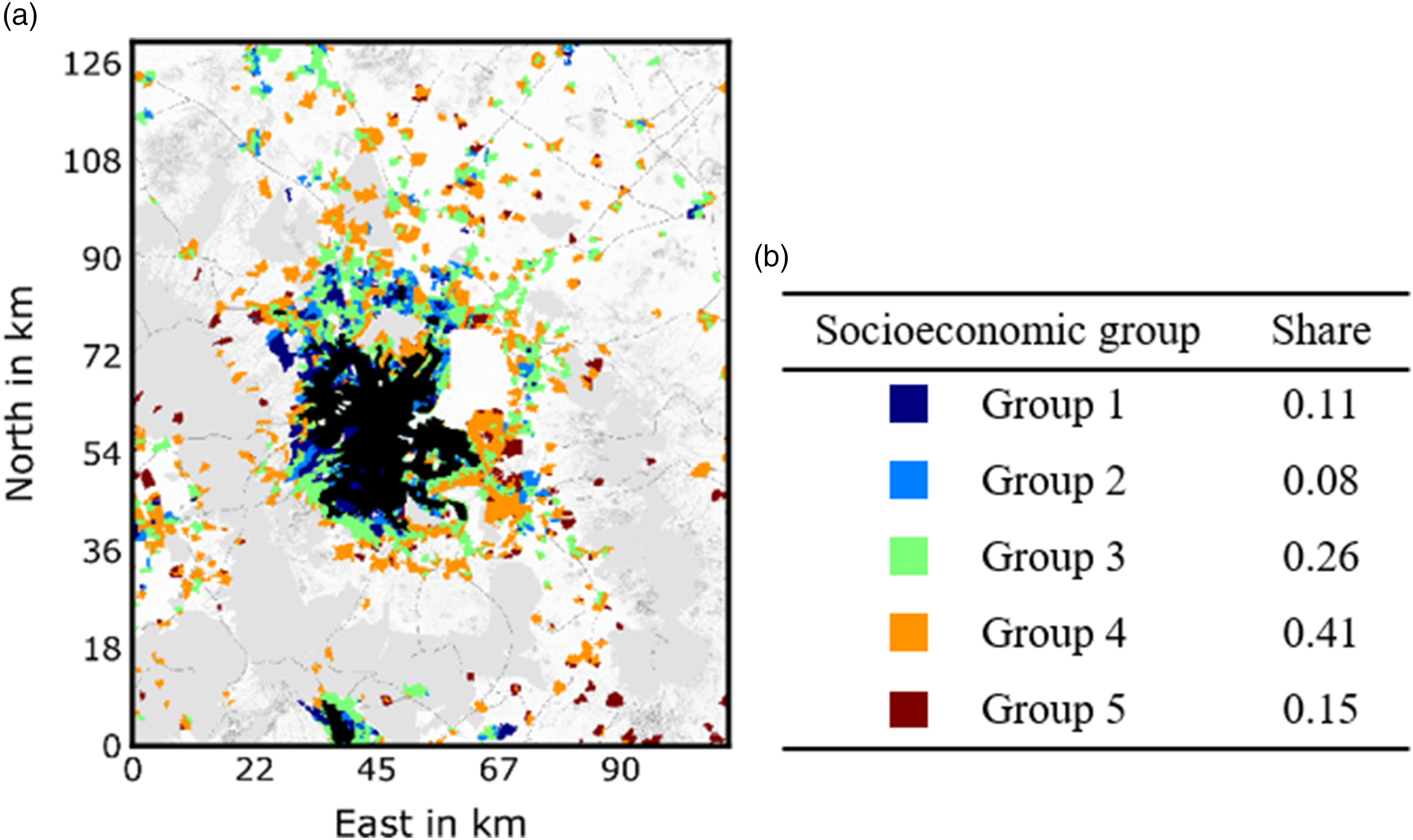

Environmental characteristics as features

A total of 16 features are used for characterizing the environment. These are: elevation, slope, aspect, protected or excluded areas, land use, climatology, flood risk, drought risk, soil degradation, toxicity, distance to wells (based on the wells dataset), distance to residual water treatment plants (based on the wastewater dataset), distance to water bodies (based on the land use dataset), distance to main highways (based on the roads dataset), distance to the urban core of 1997 (based on the land use dataset), and closest socioeconomic group (based on the IMU dataset). The layers for slope and aspect are calculated from the digital elevation model (DEM). The urban core layers with distance measures towards wells, residual water, main highways and an urban built-up area from 1997 are created by calculating the distance between any cell and the respective points of interest from the raw datasets. The closest socioeconomic group is extracted from the IMU of year 2000 through the nearest-neighbor algorithm. All other features were obtained directly from the raw datasets in Table 1. Supplemental Figure S4 in the Supplementary Material shows selected maps of the environmental features used in this work.

Input data for P2

Similarly to the SLEUTH model, we use the layers Slope, Land use, Excluded, Urban, and Transport. The built-up area of 1997 is used as the urban seed and only the main highways, already present in 1985, are regarded as drivers of urbanization. Inner-city transport networks are not considered. Supplemental Figure S5 in the Supplementary Material shows the input layers for simulating urban growth.

Implementation and evaluation

P1: Learning the value of land

Implementation

We use the cells urbanized during the period 2000–2005 to train the RFR model which, in turn, is used to predict the socioeconomic group of cells urbanized during 2005–2010. The learning and prediction processes of the RFR model are implemented in the Python module scikit-learn (version 0.20.2) (Pedregosa et al., 2011).

The main parameters for RFRs are the size of the feature subset that is considered for splitting a node (set as the square root of the number of features), the number of trees in the forest and the maximum depth of a tree. We apply a grid search approach with fivefold cross validation for the parameter selection of the latter two parameters. This means, we iterate over possible combinations of a set of parameters (ranging from 50 to 200 with a step size of 50), determine their accuracy with five randomly split training and validation sets and choose the regressor with the highest average score (Izenman 2008).

Based on the first model output from all features, we remove the least important ones with a low contribution in the RFR for explaining the training data. The applied feature importance takes into account the depth of a feature in the decision trees and the mean decrease in impurity that is achieved by its splits.

Evaluation

The learning data set, that is, the cells urbanized during the period 2000–2005, is divided into a training and a test set with a 80:20 split. The resulting RFR model is used to predict the socioeconomic group of the cells urbanized during the period 2005–2010. We use four metrics to evaluate the goodness of fit of our regressor for both data sets (James et al., 2013; Zhang et al., 2019). These are: mean squared error, MSE, coefficient of determination, R², accuracy, A_L, and precision, P_L. Additionally a confusion matrix summarizes the performance of the regression algorithm. Details on the calculation of these measures are found in the Supplementary Material.

P2: Simulating urban growth

Implementation

The Python-based urban growth model is available at (Molar-Cruz and Pöhler, 2020). Neighborhood interactions are simulated with a 3 × 3 kernel neighborhood (Moore), a common window size for CA models Mustafa et al. (2018); Liao et al. (2016). This results in a 270 m x 270 m moving window, more or less the size of a block. We use the urban extent from 1997 (INE 1997) as initial urban seed and simulate the urban growth until 2010. The growth coefficients controlling the behavior of the CA urban growth model are adjusted by a grid search optimization that maximizes the spatial fit to the historic urban extent while limiting the gained urban land to the historic values observed in snapshots for the years 2000, 2005, and 2010 (CONAPO 2010).

Evaluation

The goodness of fit of the urban growth model can be evaluated with different metrics (Dietzel and Clarke 2007). We use the Lee-Sallee index as primary metric. This shape index measures the accuracy or spatial fit between the model’s growth and the known urban extent for the control years (Ayazli 2019).

P3: Distributing socioeconomic groups

Implementation

The fraction of urban extent by socioeconomic group used for the stratification of urbanized cells by socioeconomic level follows the average distribution observed in Greater Mexico City during the period 2000–2010. This distribution is presented in Figure 2(b).

Evaluation

The analysis of the correctly predicted socioeconomic group is determined by the accuracy of the distribution, A_D. This is calculated as the fraction of newly urbanized cells with a correctly simulated corresponding socioeconomic group.

Results

P1: Learning the value of land

RFR training: 2000–2005

We train a RFR using the cells urbanized during the period 2000–2005, a total of 32 712 samples. The socioeconomic level of each cell is used as label and 16 environmental characteristics as predictors. We found out that the RFR with 100 trees and a maximum depth of 100 with a fivefold cross-validated R² = 0.97 (± 0.00), 95% confidence interval in brackets, has the best performance. The resulting feature importance is shown in Figure 3(a) ordered by decreasing importance. Only the seven features with the highest contribution, indicated with the extent of the horizontal line in the x-axis, are used for generating the land value map in Figure 3(b). This map is calculated by evaluating the RFR model with the reduced set of predictors for each cell of 90 m by 90 m in the study area.

Figure 3.

Results of the RFR for Greater Mexico City: (a) Feature importance in descending order and (b) the resulting land value map.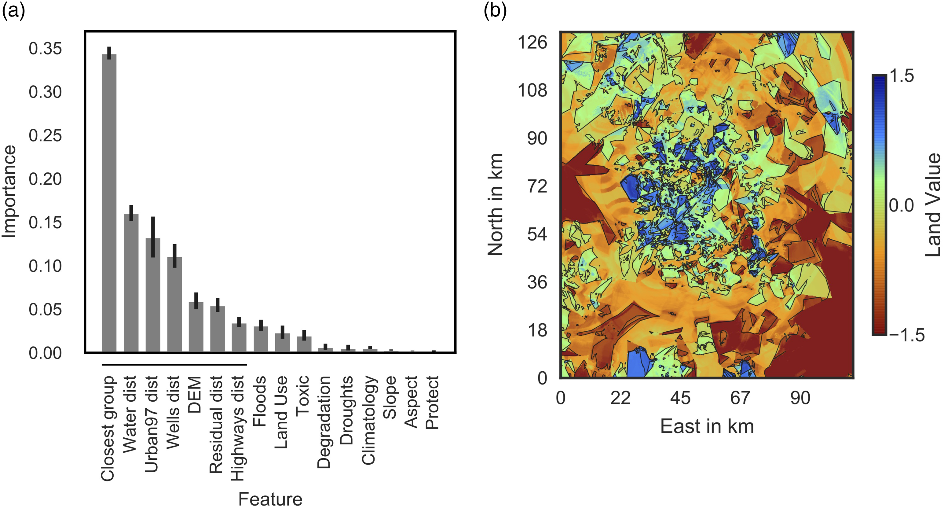

Our results show that the closest socioeconomic group in 2000 is the most influencing feature followed by the distance to water bodies (derived from the land use map) and the distance to the urban core area of 1997. This suggests that the newly urbanized cells are likely to settle in neighborhoods of a similar socioeconomic group already existing in 2000. Moreover, the distance to the urban center leads to a declining predicted socioeconomic level of the settlements and thus to a lower land value. Areas with the lowest land value in southern Greater Mexico City, a region with high mountainous ridges, show the influence of elevation. However, we observe that there are areas with a high land value that are also found far away from the urban core and within the high-elevation region. Here, the distance to water bodies, associated with the existence of green spaces, and thus, to superior ecosystem services, may have an influence on the value of land. These findings are in accordance with the results of other studies in cities of developing countries (Azhdari et al., 2018; Duque et al., 2019; García-Ayllón 2016). Environmental features that negatively impact the value of land such as the degree of drought risk, the degree of flood risk, or toxicity hazard, are low importance features and are not directly considered for the generation of the land value map, as their influence could be correlated with other characteristics already taken into account. For instance, Mexico City has serious problems managing flood risk and water scarcity affecting irregular low-income settlements in the southeastern part of the city (Eakin et al., 2016). This is well captured in the land value map with reduced features in Figure 3(b) since drought and flood risk are correlated with DEM and distance to water bodies.

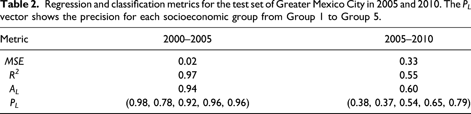
The average accuracy, A_L, of the RFR to predict the socioeconomic level of new settlements between 2000 and 2005 based on the seven environmental features is of 94% (see Table 2). The confusion matrix in Figure 4(a) compares the expected against the predicted socioeconomic level in the test set (20% of the data) and shows that overall, the model fits the true data.

Table 2.

Regression and classification metrics for the test set of Greater Mexico City in 2005 and 2010. The P_L vector shows the precision for each socioeconomic group from Group 1 to Group 5.

Metric	2000–2005	2005–2010
MSE	0.02	0.33
R ²	0.97	0.55
A _L	0.94	0.60
P _L	(0.98, 0.78, 0.92, 0.96, 0.96)	(0.38, 0.37, 0.54, 0.65, 0.79)

Figure 4.

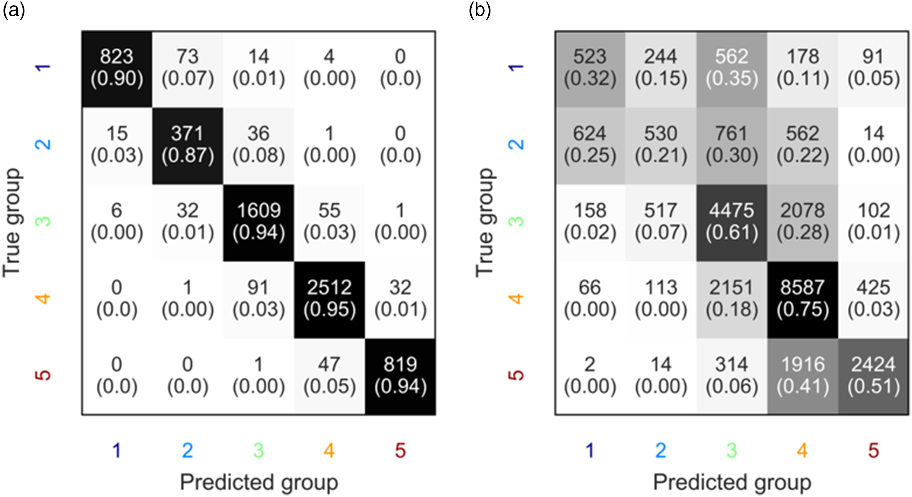
Confusion matrices for the (a) RFR training (2000–2005) and (b) prediction (2005–2010) of the socioeconomic status of newly urbanized cells. The numbers in each box represent the absolute number of cells whereas the values in brackets display the ratio in the row direction. The color of the cell represents the density estimation of the prediction.

Evaluating 2005–2010

The trained RFR for the new settlements created between 2000 and 2005 is used to predict the socioeconomic group of the cells urbanized in 2005–2010 with a total of 27431 samples. The evaluation metrics for the periods 2000–2005 and 2005–2010 are summarized in Table 2. Moreover, the prediction performance of the RFR model is visualized in the confusion matrix in Figure 4(b). In most cases, the algorithm correctly classifies the majority of the new urban cells of Groups 3, 4, and 5. However, the performance is rather poor for Groups 1 and 2. This confusion is to be expected as the IMU, used as proxy for socioeconomic status, measures social deprivation and not the real value of land. Social deprivation is correlated with income (Chan and Wong 2020) and, therefore, with purchasing power. Yet, this relationship is better adjusted for low-income groups rather than high-income groups. Nevertheless, we achieve an overall accuracy of 60%.

P2: Simulating urban growth

Using as initial urban seed the built-up area of 1997, the urban growth is simulated up to 2010. A simulation horizon of 13 years (60 simulation cycles) leads to a total of 363 130 urban cells in 2010 with a Lee-Salle index of 42%. The growth coefficients resulting from the grid search optimization are presented in Table 3. The top part of Figure 5 shows the resulting urban structure by growth type for three snapshots: 2000, 2005 and 2010. It is observed that the majority of urbanized cells result from edge growth. Road-influenced growth, visible in green near the main highways, is the second contributor. The main difference observed when comparing the historic snapshot of 2010 (Figure 2(a)) against the simulation for the same year (Figure 5(c)), is that the urban growth near the centroid is lower than expected while that of the satellite urban centers is higher. This is due to the fact that in reality, organic growth (edge growth) is not homogeneous throughout the study area and it tends to decrease with increasing distance from the core city. This behavior is not captured by the CA model as it uses a constant spread coefficient k_spread to simulate the edge growth for the whole study area. Nonetheless, the location of urban centers spatially coincides in both Figures resulting in a fragmented and sparse pattern of urban growth, common in growing cities in developing countries (Duque et al., 2019; Leao et al., 2004).

Table 3.

Growth coefficients for CA model for a simulation horizon of 13 years in 60 growth cycles of equal length.

Coefficient	Value
k_dispersion	0.15
k_breed	0.35
k_spread	0.50
k_slopeResistance	0.60
k_roadGravity	0.35

Figure 5.

Urban growth of Greater Mexico City in the period 1997–2010 in three snapshots showing the type of growth resulting from the CA model (top) and the socioeconomic group predicted by the RFR model (bottom). The black area represents the initial urban seed in 1997.

P3: Distributing socioeconomic groups

The newly urbanized cells per growth cycle are used together with the land value map to simulate urban growth stratified by socioeconomic level. The bottom part of Figure 5 illustrates the simulated growth process with new urban cells distributed into five groups of socioeconomic levels. The reference fraction of urban extent by socioeconomic group is assumed as the average distribution for the period 2000–2010 (Table 2).

The location errors of the new urban cells resulting from the CA urban growth simulation affect the spatial distribution of high socioeconomic groups (Group 1 and 2). This is observed by comparing the bottom map in Figure 5(c) and the real distribution of socioeconomic groups in 2010 in Figure 2(a). In the case of a spatial mismatch in high land value areas, which are generally smaller than low land value areas, Groups 1 and 2 occupy the available urban cells with higher land value, displacing other groups in the process. However, given that the combined fraction of urban extent of Groups 3, 4, and 5 is almost four times larger than that of Groups 1 and 2, the results obtained do depict the intra-urban dynamics observed in Mexico City in the study period.

Discussion

Learning the value of land

The value of land is determined by the economic principle of highest and best use of land which produces the highest net return over a period. The factors that can influence the value formation have been traditionally analyzed using hedonic pricing, and implemented through multivariate linear regression techniques (Azhdari et al., 2018; Liu 2010; Morales et al., 2019). However, the inherent complexity of the value formation process together with the increasing amount of data available with a potential contribution to land value, make it necessary to develop new methods capable of dealing with such a large amount of information. Machine-learning techniques such as RFR or artificial neural networks have been used for such tasks (Berberoğlu et al., 2016; Gounaridis et al., 2019) with promising outcomes.

The RFR model used in this work results in high R²-scores when cross-validated with the historic data of year 2005. Thus, the random forest demonstrates to be a good choice for learning the dependence of the socioeconomic level of new settlements on environmental characteristics. However, the “black” box nature of this model, resulting from numerous decision trees, makes it difficult to interpret the results. We calculate the feature importance as a simple way to identify which features are most predictive of the socioeconomic status. However, how these features influence prediction is not explicitly shown, although this can be inferred to some extent. Additional models such as Partial Least Squares Regression and methods for interpretation can be used for a better understanding of the contribution of each feature (Kuhn and Johnson 2013; Molnar 2021).

Implications on urban planning and urban sustainability

Models capable of simulating urban growth and the spatial distribution of socioeconomic groups are useful tools for understanding the urbanization process and project its spatio-temporal dynamics. Furthermore, such tools can also be used to project possible urban futures based on macroeconomic conditions or urban planning strategies. In addition to the already known benefits of these projections in urban policy development, they also provide useful information for assessing the sustainability implications of urbanization.

As an example, knowing the socioeconomic group that is likely to settle at a specific location is a first step towards anticipating the demand for urban services, including energy and water supply, transportation, food, communication, etc., since the amount of resources needed depends to a large extent on the consumption habits of the city’s inhabitants, which are often dictated by their purchasing power. This allows local governments to anticipate new urban population and thus plan the provision of public services and the efficient use of resources. In this way, urban policies can also promote city productivity and urban sustainability while reducing intra-urban social inequality and the resulting spatial mismatch.

Limitations and further research directions

We identify four main limitations of our approach. First, we neglect the population density and, therefore, distribute the socioeconomic groups according to the number of urbanized cells based on the fraction of urban extent they occupy. This is a strong assumption, as regions that are based on different housing types can have diverse population densities.

Second, we do not consider any additional internal urbanization process such as the recontextualization of city areas and their upgrading. This would lead to a changing land value over time. A static land value map might not completely capture the urban dynamics. An additional assessment of the factors influencing the upgrading or downgrading of existing settlements would be necessary to include them in our approach.

Third, we assume that the demographic and economic factors at the macro-scale affecting the urbanization process of the city for a specific period are known. This information is used to calibrate the CA model and to distribute the urbanized cells into five socioeconomic groups. If this approach were to be used to forecast urban growth, scenarios of macroeconomic and urban policy conditions would have to be formulated to define the urbanization path and the expected distribution of socioeconomic groups for the entire city.

Finally, we also assume that the settlers comply with the rules for protected areas and thus, our excluded layer is binary. Nonetheless, illegal settlements are sometimes also developed in protected areas (Aguilar 2008; Azhdari et al., 2018). To resolve this limitation, a data-driven approach could be used to determine the probability of settling illegally per socioeconomic group.

Conclusion

The integration of a machine-learned land value map to predict the socioeconomic status of new urban cells as a post-processing step of the CA urban growth model is a simple but effective approach to simulate both urban growth and the socioeconomic group likely to settle. We took advantage of the transparency and simplicity of the widely-used SLEUTH model to simulate the urban growth of Greater Mexico City during the period 1997–2010. A random forest regressor was used to generate a land value map of the newly urbanized cells from 2000 to 2005 based on seven environmental features. We used this map to determine the socioeconomic group of the cells urbanized up to the year 2010, the end of the study period, with an overall accuracy of 60%. In this way, we were able to model the intra-urban structure, resulting from the uneven spatial distribution of social groups within the city.

Our results showed that most of the urban growth in Greater Mexico City comes from edge growth, which simulates the organic outward spread of the city at its edges. Regarding the land value map, we found that the closest socioeconomic group in 2000 has the strongest contribution followed by the distance to water bodies and the distance to the urban center. This suggests that the newly urbanized cells are likely to settle in neighborhoods of similar socioeconomic level. Moreover, the increasing distance from the urban center resulted in a general decreasing land value. However, regions with a high land value were also found in remote areas where environmental features that improve the ecosystem services were also present.

This work can serve as a tool to support the creation of urban policies for growing cities in developing countries that promote city productivity and urban sustainability while reducing intra-urban social inequality and the resulting spatial mismatch.

Supplemental Material

sj-pdf-1-epb-10.1177_23998083211056957 – Supplemental Material for Who settles where? Simulating urban growth and socioeconomic level using cellular automata and random forest regression

Supplemental Material, sj-pdf-1-epb-10.1177_23998083211056957 for Who settles where? Simulating urban growth and socioeconomic level using cellular automata and random forest regression by Anahi Molar-Cruz, Lukas D Pöhler, Thomas Hamacher and Klaus Diepold in Environment and Planning B: Urban Analytics and City Science

Footnotes

Acknowledgements

The authors are grateful to the anonymous reviewers for their constructive comments and suggestions to improve the paper.

Declaration of conflicting interests

The author(s) declared no potential conflicts of interest with respect to the research, authorship, and/or publication of this article.

Funding

The author(s) disclosed receipt of the following financial support for the research, authorship, and/or publication of this article: This research is supported by Consejo Nacional de Ciencia y Tecnología (CVU 535272).

ORCID iDs

Anahi Molar-Cruz

Lukas D. Pöhler

Supplemental material

Supplemental material for this article is available online. Processed input data and scripts are available online at (Molar-Cruz and Pöhler, 2020).

References

Aburas

Ramli

, et al. (2016) The simulation and prediction of spatio-temporal urban growth trends using cellular automata models: A review. International Journal of Applied Earth Observation and Geoinformation 52: 380–389. DOI: 10.1016/j.jag.2016.07.007.

Agarwal

Green

Grove

, et al. (2002) A Review and Assessment of Land-Use Change Models: Dynamics of Space, Time, and Human Choice. London, UK: Apollo The International Magazine Of Art And Antiques. http://citeseerx.ist.psu.edu/viewdoc/download?doi=10.1.1.86.2775&rep=rep1&type=pdf.

Aguilar

(2008) Peri-urbanization, illegal settlements and environmental impact in Mexico City. Cities 25(3): 133–145. DOI: 10.1016/j.cities.2008.02.003.

Almeida

Gleriani

Castejon

, et al. (2008) Using neural networks and cellular automata for modelling intra‐urban land‐use dynamics. International Journal of Geographical Information Science 22(9): 943–963. DOI: 10.1080/13658810701731168.

Ayazli

(2019) Monitoring of urban growth with improved model accuracy by statistical methods. Sustainability 11(20): 5579. DOI: 10.3390/su11205579.

Azhdari

Sasani

Soltani

(2018) Exploring the relationship between spatial driving forces of urban expansion and socioeconomic segregation: The case of Shiraz. Habitat International 81: 33–44. DOI: 10.1016/j.habitatint.2018.09.001.

Barros

(2004) Urban Growth in Latin American Cities: Exploring Urban Dynamics through Agent-Based Simulation. Doctoral. London, UK: University of London. https://discovery.ucl.ac.uk/id/eprint/1369523.

Batty

(2012) Building a science of cities. Cities 29: S9S16–S16. DOI: 10.1016/j.cities.2011.11.008.

Batty

Longley

(1994) Fractal Cities - A Geometry of Form and Function. London, UK: Academic Press.

10.

Berberoğlu

Akın

Clarke

(2016) Cellular automata modeling approaches to forecast urban growth for adana, Turkey: A comparative approach. Landscape and Urban Planning 153: 11–27. DOI: 10.1016/j.landurbplan.2016.04.017.

11.

Bonilla-Bedoya

Mora

Vaca

, et al. (2020) Modelling the relationship between urban expansion processes and urban forest characteristics: an application to the metropolitan district of Quito. Computers, Environment and Urban Systems 79(15): 101420. DOI: 10.1016/j.compenvurbsys.2019.101420.

12.

Broxton

Zeng

Sulla-Menashe

, et al. (2014) A global land cover climatology using MODIS data. Journal of Applied Meteorology and Climatology 53(6): 1593–1605. DOI: 10.1175/JAMC-D-13-0270.1.

13.

CENAPRED (2007) Grado de riesgo por inundaciones por municipio. Tlalpan, Mexico: CONABIO. http://www.conabio.gob.mx/informacion/metadata/gis/grinundmgw.xml.

14.

CENAPRED (2012a) Grado de peligro por sequía por municipio. Tlalpan, Mexico: CONABIO. http://www.conabio.gob.mx/informacion/metadata/gis/pelsequigw.xml?_httpcache=yes&_xsl=/db/metadata/xsl/fgdc_html.xsl&_indent=no.

15.

CENAPRED (2012b) Índice de peligro por sustancias tóxicas por municipio. Tlalpan, Mexico: CONABIO. http://www.conabio.gob.mx/informacion/gis/?vns=gis_root/riesgo/riequimico/ipsusttoxgw.

16.

Chan

Wong

(2020) Impact of income, deprivation and social exclusion on subjective poverty: a structural equation model of multidimensional poverty in Hong Kong. Social Indicators Research 152(3): 971–990. DOI: 10.1007/s11205-020-02476-8.

17.

Clarke

Hoppen

Gaydos

(1997) A self-modifying cellular automaton model of historical urbanization in the San Francisco Bay area. Environment and Planning B: Planning and Design 24(2): 247–261. DOI: 10.1068/b240247.

18.

CONABIO (2015) Áreas Naturales Protegidas Estatales, Municipales, Ejidales y Privadas de México. Tlalpan, Mexico: CONABIO. http://www.conabio.gob.mx/informacion/gis/?vns=gis_root/region/biotic/anpest15gw.

19.

CONANP (2017) Áreas Naturales Protegidas Federales de México. Tlalpan, Mexico: CONABIO. http://www.conabio.gob.mx/informacion/gis/?vns=gis_root/region/biotic/anpnov17gw.

20.

CONAPO (2010) Índice de Marginación Urbana. Mexico City, Mexico: CONAPO. http://www.conapo.gob.mx/es/CONAPO/Indices_de_Marginacion.

21.

Dietzel

Clarke

(2007) Toward optimal calibration of the SLEUTH land use change model. Transactions in GIS 11(1): 29–45. DOI: 10.1111/j.1467-9671.2007.01031.x.

22.

Dig Chart of the World (1985) Red de carreteras. Tlalpan, Mexico: CONABIO. http://www.conabio.gob.mx/informacion/gis/?vns=gis_root/infra/vcomun/carre1mgw.

23.

Duque

Lozano-Gracia

Patino

, et al. (2019) Spatiotemporal dynamics of urban growth in Latin American cities: an analysis using nighttime light imagery. Landscape and Urban Planning 191(12): 103640. DOI: 10.1016/j.landurbplan.2019.103640.

24.

Eakin

Lerner

Manuel-Navarrete

, et al. (2016) Adapting to risk and perpetuating poverty: household’s strategies for managing flood risk and water scarcity in Mexico City. Environmental Science & Policy 66: 324–333. DOI: 10.1016/j.envsci.2016.06.006.

25.

Frenkel

Israel

(2018) Spatial inequality in the context of city-suburb cleavages-enlarging the framework of well-being and social inequality. Landscape and Urban Planning 177: 328–339. DOI: 10.1016/j.landurbplan.2017.02.018.

26.

García-Ayllón

(2016) Rapid development as a factor of imbalance in urban growth of cities in Latin America: a perspective based on territorial indicators. Habitat International 58: 127–142. DOI: 10.1016/j.habitatint.2016.10.005.

27.

Gounaridis

Chorianopoulos

Symeonakis

, et al. (2019) A random forest-cellular automata modelling approach to explore future land use/cover change in Attica (Greece), under different socio-economic realities and scales. Science of the Total Environment 646: 320–335. DOI: 10.1016/j.scitotenv.2018.07.302.

28.

(2019) Urbanization: processes and driving forces. Science China Earth Sciences 62(9): 1351–1360. DOI: 10.1007/s11430-018-9359-y.

29.

Guzman

Escobar

Peña

, et al. (2020) A cellular automata-based land-use model as an integrated spatial decision support system for urban planning in developing cities: the case of the Bogotá region. Land Use Policy 92(3): 104445. DOI: 10.1016/j.landusepol.2019.104445.

30.

Houet

Aguejdad

Doukari

, et al. (2016) Description and validation of a “non-path-dependent” model for projecting contrasting urban growth futures. CyberGeo 759. DOI: 10.4000/cybergeo.27397.

31.

INE (1997) Uso Del Suelo Y Vegetación. Tlalpan, Mexico: CONABIO. http://www.conabio.gob.mx/informacion/gis/?vns=gis_root/usv/inegi/usv250kcs1agw.

32.

INEGI (2015) Directorio Estadístico Nacional de Unidades Ecónomicas (DENUE) - Actividad Económicas. Aguascalientes City, Aguascalientes: Instituto Nacional de Estadística, Geografía e Informatica. https://www.inegi.org.mx/app/descarga/?ti=6.

33.

Izenman

(2008) Modern Multivariate Statistical Techniques. New York, NY: Springer Texts in StatisticsSpringer. DOI: 10.1007/978-0-387-78189-1.

34.

Jaitman

(2015) Urban infrastructure in Latin America and the Caribbean: public policy priorities. Latin American Economic Review 24(1): 13. DOI: 10.1007/s40503-015-0027-5.

35.

James

Witten

Hastie

, et al. (2013) An Introduction to Statistical Learning, Springer Texts in Statistics. New York, NY: Springer, 103. DOI: 10.1007/978-1-4614-7138-7.

36.

Jean

Burke

Xie

, et al. (2016) Combining satellite imagery and machine learning to predict poverty. Science 353(6301): 790–794. DOI: 10.1126/science.aaf7894.

37.

Jedwab

Christiaensen

Gindelsky

(2017) Demography, urbanization and development: rural push, urban pull and … urban push? urban push?. Journal of Urban Economics 98: 6–16. DOI: 10.1016/j.jue.2015.09.002.

38.

Kamusoko

Aniya

Adi

, et al. (2009) Rural sustainability under threat in Zimbabwe - simulation of future land use/cover changes in the Bindura district based on the Markov-cellular automata model. Applied Geography 29(3): 435–447. DOI: 10.1016/j.apgeog.2008.10.002.

39.

Kuhn

Johnson

(2013) Applied Predictive Modelling. New York, NY: Springer. DOI: 10.1007/978-1-4614-6849-3.

40.

Leao

Bishop

Evans

(2004) Simulating urban growth in a developing nation’s region using a cellular automata-based model. Journal of Urban Planning and Development 130(3): 145–158. DOI: 10.1061/(asce)0733-9488.

41.

Yeh

AG-O

(2002) Neural-network-based cellular automata for simulating multiple land use changes using gis. International Journal of Geographical Information Science 16(4): 323–343. DOI: 10.1080/13658810210137004.

42.

Liao

Tang

Shao

, et al. (2016) Incorporation of extended neighborhood mechanisms and its impact on urban land-use cellular automata simulations. Environmental Modelling & Software 75: 163–175. DOI: 10.1016/j.envsoft.2015.10.014.

43.

Batty

(2010) Modelling urban development with geographical information systems and cellular automata. The Photogrammetric Record 25: 320–323. DOI: 10.1111/j.1477-9730.2010.00593.x.

44.

Lyu

Zhang

, et al. (2019) Modeling the effects of urban expansion on regional carbon storage by coupling SLEUTH‐3r model and InVEST model. Ecological Research 34(3): 380–393. DOI: 10.1111/1440-1703.1278.

45.

Molar-Cruz

Pöhler

(2020) Intus: Modeling Integrated Urban Systems. San Francisco, CA: GitHub. Available at: https://github.com/tum-ens/intus/tree/ca_land_value.

46.

Molnar

(2021) Interpretable Machine Learning: A Guide for Making Black Box Models Explainable. San Francisco, CA: GitHub. https://christophm.github.io/interpretable-ml-book/.

47.

Morales

Flacke

Zevenbergen

(2019) Modelling residential land values using geographic and geometric accessibility in guatemala city. Environment and Planning B: Urban Analytics and City Science 46(4): 751–776. DOI: 10.1177/2399808317726332.

48.

Mustafa

Heppenstall

Omrani

, et al. (2018) Modelling built-up expansion and densification with multinomial logistic regression, cellular automata and genetic algorithm. Computers, Environment and Urban Systems 67(2): 147–156. DOI: 10.1016/j.compenvurbsys.2017.09.009.

49.

NASA JPL (2013) NASA Shuttle Radar Topography Mission Global 1 Arc Second. Washington, DC: LP DAAC. https://lpdaac.usgs.gov/products/srtmgl1v003/.

50.

Ntinas

Moutafis

Trunfio

, et al. (2017) Parallel fuzzy cellular automata for data-driven simulation of wildfire spreading. Journal of Computational Science 21: 469–485. DOI: 10.1016/j.jocs.2016.08.003.

51.

Paiva

ACdE

Nascimento

Rodriguez

, et al. (2020) Urban expansion and its impact on water security: the case of the Paraíba do Sul River Basin, São Paulo, Brazil. Science of the Total Environment 720: 137509. DOI: 10.1016/j.scitotenv.2020.137509.

52.

Pedregosa

Varoquaux

Gramfort

, et al. (2011) Scikit-learn: machine learning in python. Journal of Machine Learning Research 12: 2825–2830. DOI: 10.1007/s13398-014-0173-7.2.

53.

Reardon

O'Sullivan

(2004) 3. Measures of Spatial Segregation. Sociological Methodology 34(650): 121–162. DOI: 10.1111/j.0081-1750.2004.00150.x.

54.

Rienow

Goetzke

(2015) Supporting SLEUTH - enhancing a cellular automaton with support vector machines for urban growth modeling. Computers, Environment and Urban Systems 49: 66–81. DOI: 10.1016/j.compenvurbsys.2014.05.001.

55.

Santos

Polidori

Peres

, et al. (2014) Hybrid cellular automaton —agent-based model of informal peripheral development in Latin American Cities. In: 21st International Seminar on Urban Form: Our common future in Urban Morphology. Porto, Portugal, 15 November 2014.

56.

SEMARNAT-CP (2004) Degradación del suelo en la República Mexicana. Tlalpan, Mexico: Conabio. http://www.conabio.gob.mx/informacion/gis/?vns=gis_root/edafo/dsuelo/degra250kgw.

57.

UN Department of Economic and Social Affairs (2018) World Urbanization Prospects: The 2018 Revision. New York, NY: Technical report, UN. https://population.un.org/wup/Publications/Files/WUP2018-Report.pdf.

58.

UN Population Division (2018) The World’s Cities in 2018. New York, NY: Data Booklet. https://digitallibrary.un.org/record/3799524/files/the_worlds_cities_in_2018_data_booklet.pdf.

59.

Vermeiren

Vanmaercke

Beckers

, et al. (2016) ASSURE: a model for the simulation of urban expansion and intra-urban social segregation. International Journal of Geographical Information Science 30(12): 2377–2400. DOI: 10.1080/13658816.2016.1177641.

60.

White

(1983) The measurement of spatial segregation. American Journal of Sociology 88(5): 1008–1018. DOI: 10.1086/227768.

61.

Liu

Wang

, et al. (2010) Simulating urban expansion by coupling a stochastic cellular automata model and socioeconomic indicators. Stochastic Environmental Research and Risk Assessment 24(2): 235–245. DOI: 10.1007/s00477-009-0313-3.

62.

Wurm

Stark

Zhu

, et al. (2019) Semantic segmentation of slums in satellite images using transfer learning on fully convolutional neural networks. ISPRS Journal of Photogrammetry and Remote Sensing 150: 59–69. DOI: 10.1016/j.isprsjprs.2019.02.006.

63.

Zhang

Huettmann

Zhang

, et al. (2019) The use of classification and regression algorithms using the random forests method with presence-only data to model species’ distribution. MethodsX 6: 2281–2292. DOI: 10.1016/j.mex.2019.09.035.

64.

Zhao

Liu

, et al. (2019) Estimation of poverty using random forest regression with multi-source data: a case study in Bangladesh. Remote Sensing 11(4): 375. DOI: 10.3390/rs11040375.

Supplementary Material

Please find the following supplemental material available below.

For Open Access articles published under a Creative Commons License, all supplemental material carries the same license as the article it is associated with.

For non-Open Access articles published, all supplemental material carries a non-exclusive license, and permission requests for re-use of supplemental material or any part of supplemental material shall be sent directly to the copyright owner as specified in the copyright notice associated with the article.

0.00 MB

3.91 MB