Minimizing aggregation errors when measuring potential access to services for social groups at the city scale

Abstract

This research explores how to minimize aggregation errors when measuring potential access to services for social groups at the city scale. It develops a cadastral and address-based population weighting technique, the Household Space Weighting, to reduce aggregation errors caused by using population weighted centroids when applying the Have Their Centre In criterion (the Population Weighted Centroid technique). The Household Space Weighting technique is formally tested in a case study of General Practitioner practices in Newcastle upon Tyne, UK. The findings suggest that the Population Weighted Centroid technique produces inaccurate population estimates for 267 out of 910 output areas (29%) in the city. When applying the two techniques to measure access for social groups at the city scale, the absolute difference in the percentage of each social group with potential accessibility is 9–10% and the relative difference in the percentage of each social group with potential access is 18–20%, taking into account the overlay of service areas at the city scale. This suggests that if service planners or policy makers want to measure potential accessibility or potential access of social groups to services for cities, it would be useful to apply a more accurate technique, or at least be aware of the implications of applying the Population Weighted Centroid technique.

Introduction

The ecological fallacy, Modifiable Areal Unit Problem and aggregation errors

Individual or household-level data are not available in many countries due to privacy, confidentiality and other considerations; thus, statistical or census data are normally aggregated and reported for areal units (AUs) (Apparicio et al., 2008; Hewko et al., 2002; Heynen et al., 2006; Landry and Chakraborty, 2009; Openshaw, 1984; Tooke et al., 2010). It has long been recognized that using aggregate data to refer to individual characteristics within statistical analysis causes ‘ecological fallacy’ (Baldwin, 1974; Daras and Alvanides, 2006; Giggs, 1973; Johnston, 1976; Openshaw, 1984). For example, Robinson’s (2009) research concluded that ecological and individual correlations are not equal and the former cannot validly be used as a substitute for the latter.

Geographical analysis using AUs combined with statistical or census data reporting individual characteristics causes the Modifiable Areal Unit Problem (MAUP), a special form of ‘ecological fallacy’, when AUs are modified in the sense as if they could be aggregated or disaggregated (Daras and Alvanides, 2006). One related component, the zoning (or aggregation) problem, is associated with any changes in results caused by alternative AUs of analysis where the number of AUs is invariable (Jelinski and Wu, 1996; Openshaw and Taylor, 1979). In terms of measuring access, aggregation errors occur when the centroid is used to represent the AU as it assumes that populations within the AU are homogeneous and evenly distributed (Apparicio et al., 2008; Smoyer-Tomic et al., 2004), which does not reflect reality due to stochastic or random processes (Jones et al., 2018).

To reduce aggregation errors, there are spatial disaggregation techniques (e.g. dasymetric mapping) which intend to identify the location of the population by locating residential buildings in the absence of household-level census data. There are also other techniques to improve spatial representation of AUs, such as the technique using population weighted centroids (PWCs) to replace geographic centroids (GCs) of AUs, which takes into consideration the location of households (ONS, 2013). These techniques will be discussed in detail in the next subsection.

Potential accessibility and potential access, place access and population access

Potential accessibility (PAB) represents the interaction between the location of potential population and the service as a distance-based concept. Potential access (PA) refers to the ‘availability of that service moderated by space, or the distance variable’ in the health-related literature (Khan, 1992: 275). Thus, from a spatial perspective, access to healthcare services contains both availability (such as the number of physicians or full-time equivalent (FTE) physicians, e.g. Khan, 1992; Luo and Wang, 2003) and accessibility (Andersen et al., 1983; Figueroa et al., 2001; Khan, 1992; Penchansky and Thomas, 1981). For both PAB and PA, spatial representation and the scale of analysis are important as they affect results generated and, ultimately, policy implications of findings (Crawford, 2006; Goodchild, 2011; Wu and Li, 2006).

Place access is related to the use of centroids to represent AUs when measuring access; population access is associated with the actual location of the population and its subgroups when measuring access (Talen, 2003). Due to the unavailability of household-level census data, most studies use a place access rather than a population access measurement method.

For better spatial representation, PWCs were introduced to replace GCs (e.g. Higgs and White, 2000; Wang and Luo, 2005). PWCs are used in UK policy documents, such as the English Indices of Deprivation 2015 (DCLG, 2015) to measure accessibility to key local services (e.g. post offices, primary schools, general stores or supermarkets and General Practitioner (GP) practices). The replacement of GCs by PWCs makes spatial representation more accurate and closer to reality because the median centroid algorithm used in the calculation of PWCs takes into consideration the location of households (ONS, 2013). Thus, when applying the Have Their Centre In criterion to measure access, the result will be more accurate using PWCs (i.e. the PWC technique) than using GCs. For instance, Apparicio et al.’s (2008) research compares aggregation errors caused by using census tract centroids, population-weighted mean for dissemination areas within census tracts and population-weighted mean for blocks within census tracts. The results of the research indicate a difference in measurement errors of 5–10% from the least accurate aggregation method (using census tract centroids) to the most accurate aggregation method (using population-weighted mean for blocks within census tracts).

However, the PWC is still a single summary reference point of an AU. Aggregation errors still occur due to the use of single points to represent polygons when it is combined with the application of the Have Their Centre In criterion to measure access (Smoyer-Tomic et al., 2004). Thus, the PWC technique is still a place access rather than a population access measurement method, as it measures access for AUs using their PWCs rather than for the population and its subgroups within those AUs.

The fundamental problem with the PWC technique is its assumption that the populations within the AU are either located fully inside or outside the service area (SA). Accordingly, there is a dichotomous way of assigning weights to AUs with access when applying the PWC technique. It assigns the weight of ‘1’ to the AU with its PWC located inside the SA (i.e. full access) and the weight of ‘0’ to the AU with its PWC located outside the SA (i.e. no access), and then calculates and sums up associated populations. The dichotomous way of assigning weights to AUs with access when applying the PWC technique is the source of aggregation errors, because it is unlikely that the populations within an AU are located either fully inside or outside the SA. Rather, they are located fully or partially inside or outside the SA due to the uneven distribution of the populations and the heterogeneity of the physical environment within the AU (Crawford, 2006; Hewko et al., 2002; Knox, 1979). Therefore, there is a need to explore a population weighting technique to replace the PWC technique to measure population access that can also include partial access.

An alternative disaggregation technique and population access

In attempting to develop a population weighting technique, Maantay et al.’s (2007) research reviewed existing population weighting and areal weighting techniques. It demonstrates that population weighting techniques are more accurate than areal weighting techniques.

The dasymetric mapping technique used in the research is also subject to aggregation errors, like the choroplethic mapping technique, as it still causes abrupt transitions of boundary changes of AUs. But by using ancillary land use data with smaller AUs, the dasymetric mapping technique better reflects the true underlying geography and better visualize population patterns of the area than the choroplethic mapping technique (Holt et al., 2004; Maantay et al., 2007). The research developed a more advanced population weighting technique, the Cadastral-based Expert Dasymetric System (CEDS).

However, when the CEDS is applied to estimate population inside the SA in the case study of the research, it uses GCs to represent the lowest level AUs into which it is disaggregated (i.e. tax-lots). Thus, when the CEDS is applied to measure access, it is still a place access rather than a population access measurement method. In fact, the measurement of population access requires the identification of the location of residential buildings to obtain household-level census data. Extensive research has been undertaken in order to achieve this. For instance, Boone’s (2008) research disaggregates census data by overlaying census tracts with land use information using a dasymetric mapping approach. By doing so, census data are partitioned into the land use data to identify residential areas from the land use information. Pham et al.’s (2012) study further disaggregates census data, taking into consideration the built environment, such as buildings, alleys and yards of residential parcels from satellite images. Logan et al.’s (2019) study selects residential buildings from city open data portals against the land use data, and then evenly divides the population of the census block among those selected residential buildings to provide population estimates. Despite improvement, none of the studies managed to disaggregate census data to the household level.

Disaggregating the lowest level census data available in a city to the household level will be attempted within this paper. It will be achieved by cleansing the most up-to-date and accurate cadastral and address-based data (i.e. the UKBuildings data and the AddressBase Premium data). After cleansing, the data can be used to identify the location of residential buildings by dwelling type in use that take into account houses in multiple occupancy, i.e. the household space (HS). It can then be used to obtain the household-level census data by calculating the number of HSs to represent the number of households. By using this alternative technique, it is possible to measure the proportion of HSs within an AU located inside the SA and assign the weight to the AU with access. The resultant Household Space Weighting (HSW) technique, developed within this paper, assigns the weight of ‘1’ to the AU with all its HSs located inside the SA (i.e. full access); the weight of ‘0–1’ to the AU with parts of its HSs located inside the SA (i.e. partial access); and the weight of ‘0’ to the AU with no HS located inside the SA (i.e. no access).

As this paper intends to illustrate the measurement of PA to services in a generic way, access will be measured in the way of PAB integrating the size of services in terms of availability for reasons mentioned earlier in the previous subsection. For this, the research introduces the concept of ‘size weighting’ to measure the availability of services at the city scale, which is calculated by dividing the size of each service by the total size of the service in a city. This can also apply to services that involve physical sizes and/or numbers that have been investigated in the planning literature (such as the size of public parks or greenspaces and the number of playgrounds, e.g. Comber et al., 2008; Higgs et al., 2012; Nicholls, 2001; Omer, 2006; Smoyer-Tomic et al., 2004; Talen, 2001; Talen and Anselin, 1998).

GP practices in Newcastle upon Tyne, UK (Newcastle) will be used as a case study to illustrate and compare the application of the PWC and HSW techniques in population estimates and PAB and PA measurement for social groups at the city scale. The FTE GP will be used as an indicator to measure size; the overlay of SAs will be taken into account in the measurement because apart from the size of each service, the location of social groups inside or outside the overlay of SAs can affect the level of access. Social groups located inside the overlay of SAs have higher levels of access compared to those who located inside only one of the SAs (Luo and Wang, 2003).

Based on the above conventions, this paper develops the cadastral and address-based population weighting technique (i.e. the HSW technique) to measure population access for social groups at the city scale. The research draws upon the existing studies, particularly Maantay et al.’s (2007) research conclusion that population weighting techniques are more accurate than areal weighting techniques in population estimates and Luo and Wang’s (2003) research on how to take into account the overlay of SAs in PAB measurement. The development of the HSW technique enables further exploration into the extent of aggregation errors caused by using the PWC technique.

The next section will provide a conceptual comparison between the HSW and PWC techniques, followed by city-scale empirical comparisons. In terms of minimizing aggregation errors, this paper argues for the use of the HSW technique to replace the PWC technique in population estimates and PAB and PA measurement.

A conceptual comparison between the HSW and PWC techniques

Introduction to the four-step HSW technique

There are four steps for applying the HSW technique to measure PA to services for social groups at the city scale. The first step involves the use of GIS Network Analyst ¹ to create SAs, using a maximum walking distance threshold, drawing upon Comber et al.’s (2008) research.

The second step involves the calculation of the weight for each AU with access (i.e. full, partial or no access). This is achieved by dividing the number of HSs within an AU located inside the SA by the total number of HSs within the AU. The calculation process will be presented in equation (1)

$${\mathit{W}}_{\mathit{i}}\mathrm{=}\frac{{\mathit{N}}_{\mathit{HS}}\in \left\{{\mathit{B}}_{\mathit{A}{\mathit{U}}_{\mathit{i}}}\mathbf{\cap }{\mathit{B}}_{\mathit{S}{\mathit{A}}_{\mathit{j}}}\right\}}{{\mathit{N}}_{\mathit{HS}}\in {\mathit{B}}_{\mathit{A}{\mathit{U}}_{\mathit{i}}}}$$

(1)

where

${\mathit{W}}_{\mathit{i}}$  = The weight of ${\mathit{AU}}_{\mathit{i}}$ with access

${\mathit{N}}_{\mathit{HS}}$  = The number of HSs

${\mathit{B}}_{\mathit{A}{\mathit{U}}_{\mathit{i}}}$  = The boundary of $\mathit{A}{\mathit{U}}_{\mathit{i}}$

${\mathit{B}}_{\mathit{S}{\mathit{A}}_{\mathit{j}}}$  = The boundary of $\mathit{S}{\mathit{A}}_{\mathit{j}}$

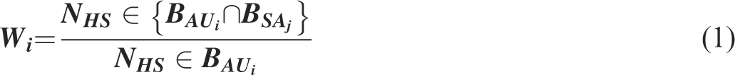
For an AU with all its HSs located inside the SA, the weight is ‘1’; for an AU with parts of its HSs located inside the SA, the weight is ‘0–1’; for an AU with no HS located inside the SA, the weight is ‘0’.

The third step involves the calculation of the number and percentage of each social group with PAB. In this step, census data reporting the characteristics of social groups are joined with the access weighting dataset in ArcGIS. ² The joined datasets are then exported to Excel ³ to calculate the number of each social group with PAB by SA, taking into account the overlay of SAs and then the total number of the social group with PAB in a city at the city scale. The calculation proces will be presented in equation (2)

$${\mathit{N}}_{\mathit{S}\mathit{G}\mathit{P}\mathit{A}{\mathit{B}}_{\mathit{c}}}\mathbf{=}\mathbf{ }\mathbf{\sum }_{\mathit{j}\mathbf{=}\mathbf{1}}^{\mathbf{m}}{\mathit{N}}_{\mathit{S}\mathit{G}\mathit{P}\mathit{A}{\mathit{B}}_{\mathit{j}}}\mathbf{ }, \mathbf{ }\mathbf{ }\mathbf{ }{\mathit{N}}_{\mathit{S}\mathit{G}\mathit{P}\mathit{A}{\mathit{B}}_{\mathit{j}}}=\mathbf{\sum }_{\mathit{i}\mathbf{=}\mathbf{1}}^{\mathbf{n}}\mathbf{(}{\mathit{N}}_{\mathbf{S}{\mathbf{G}}_{\mathit{i}}}{\mathit{W}}_{\mathit{i}}\mathbf{)}$$

(2)

where

${\mathit{N}}_{\mathit{SGP}{\mathit{AB}}_{\mathit{c}}}$  = The total number of each social group with PAB in a city, taking into account the overlay of SAs at the city scale

${\mathit{N}}_{{\mathit{SGPAB}}_{\mathit{j}}}$   = The number of each social group with PAB in ${\mathit{SA}}_{\mathit{j}}$

${\mathit{N}}_{{\mathit{SG}}_{\mathit{i}}}$  = The number of each social group within ${\mathit{AU}}_{\mathit{i}}$

${\mathit{W}}_{\mathit{i}}$  = The weight of ${\mathit{AU}}_{\mathit{i}}$ with access

The percentage of PAB is calculated by dividing the number of each social group with PAB (i.e. the numerator) by the total number of the social group involved in the calculation of PAB, taking into account the overlay of SAs at the city scale (i.e. the denominator). It is worth noting here that the number of AUs involved in the calculation of the denominator can exceed the total number of AUs in a city. This is because the HS within an AU or the PWC of an AU can locate in more than one SA when the overlay of SAs is taken into account. In this case, more than one weight may be assigned to the same AU. Calculating the percentage of each social group with PAB for each SA and then the total number of the social group with PAB in the city can ensure that the calculation process takes into account the overlay of SAs at the city scale. The calculation of the percentage of each social group with PAB will be presented in equation (3)

$${\mathit{P}}_{{\mathit{SGPAB}}_{\mathit{c}}}=\sum _{\mathit{j}\mathbf{=}\mathbf{1}}^{\mathit{m}}{\mathit{P}}_{{\mathit{SGPAB}}_{\mathit{j}}},\hspace{1em}{\mathit{P}}_{{\mathit{SGPAB}}_{\mathit{j}}}=\frac{{\mathit{N}}_{{\mathit{SGPAB}}_{\mathit{j}}}}{{\mathit{N}}_{\mathit{SG}\mathit{P}\mathit{A}{\mathit{B}}_{\mathit{c}}}}$$

(3)

where

${\mathit{P}}_{{\mathit{SGPAB}}_{\mathit{c}}}$  = The percentage of each social group with PAB in the city

${\mathit{P}}_{{\mathit{SGPAB}}_{\mathit{j}}}$  = The percentage of each social group with PAB in ${\mathit{SA}}_{\mathit{j}}$

${\mathit{N}}_{{\mathit{SGPAB}}_{\mathit{j}}}$ = The number of each social group with PAB in ${\mathit{SA}}_{\mathit{j}}$

${\mathit{N}}_{\mathit{SG}\mathit{P}\mathit{A}{\mathit{B}}_{\mathit{c}}}$ = The total number of each social group with PAB in a city, taking into account the overlay of SAs at the city scale

The fourth step is the calculation of the percentage of each social group with PA. It is calculated by multiplying the percentage of each social group with PAB by the size weighting of each related service in a city at the city scale. The size weighting is calculated by dividing the size of each service (e.g. the number of FTE GP of each GP Practice) by the total size of the service (e.g. the total number of the FTE GPs) in the city. Again, the percentage is calculated by SA and then at the city scale. The calculation process will be presented in equation (4)

$${\mathit{P}}_{{\mathit{SGPA}}_{\mathit{c}}}=\sum _{\mathit{j}=1}^{\mathit{m}}{\mathit{P}}_{{\mathit{SGPA}}_{\mathit{j}}},\hspace{1em}{\mathit{P}}_{{\mathit{SGPA}}_{\mathit{j}}}={\mathit{P}}_{{\mathit{SGPAB}}_{\mathit{j}}}\left({\mathit{S}}_{{\mathit{S}}_{\mathit{j}}}/{\mathit{S}}_{{\mathit{S}}_{\mathit{c}}}\right)$$

(4)

where

${\mathit{P}}_{{\mathit{SGPA}}_{\mathit{c}}}$  = The percentage of each social group with PA in the city

${\mathit{P}}_{{\mathit{SGPA}}_{\mathit{j}}}$  = The percentage of each social group with PA in ${\mathit{SA}}_{\mathit{j}}$

${\mathit{P}}_{{\mathit{SGPAB}}_{\mathit{j}}}$  = The percentage of each social group with PAB in ${\mathit{SA}}_{\mathit{j}}$

${\mathit{S}}_{{\mathit{S}}_{\mathit{j}}}$  = The size of service j

${\mathit{S}}_{{\mathit{S}}_{\mathit{c}}}$  = The total size of the service in the city

The conceptual presentation and comparison of the HSW to the PWC technique

This subsection will focus on the conceptual presentation and the comparison of the HSW to the PWC technique. Figure 1 shows a conceptual diagram of how to take into account the overlay of SAs in PAB measurement applying the HSW and PWC techniques at the city scale, adapting from Luo and Wang’s (2003) research. In the diagram, the rectangles represent AUs, the curved-edge polygons represent SAs, the pentagons represent HSs and the stars represent PWCs. To simplify the illustration, one pentagon will be counted as one HS.

Figure 1.

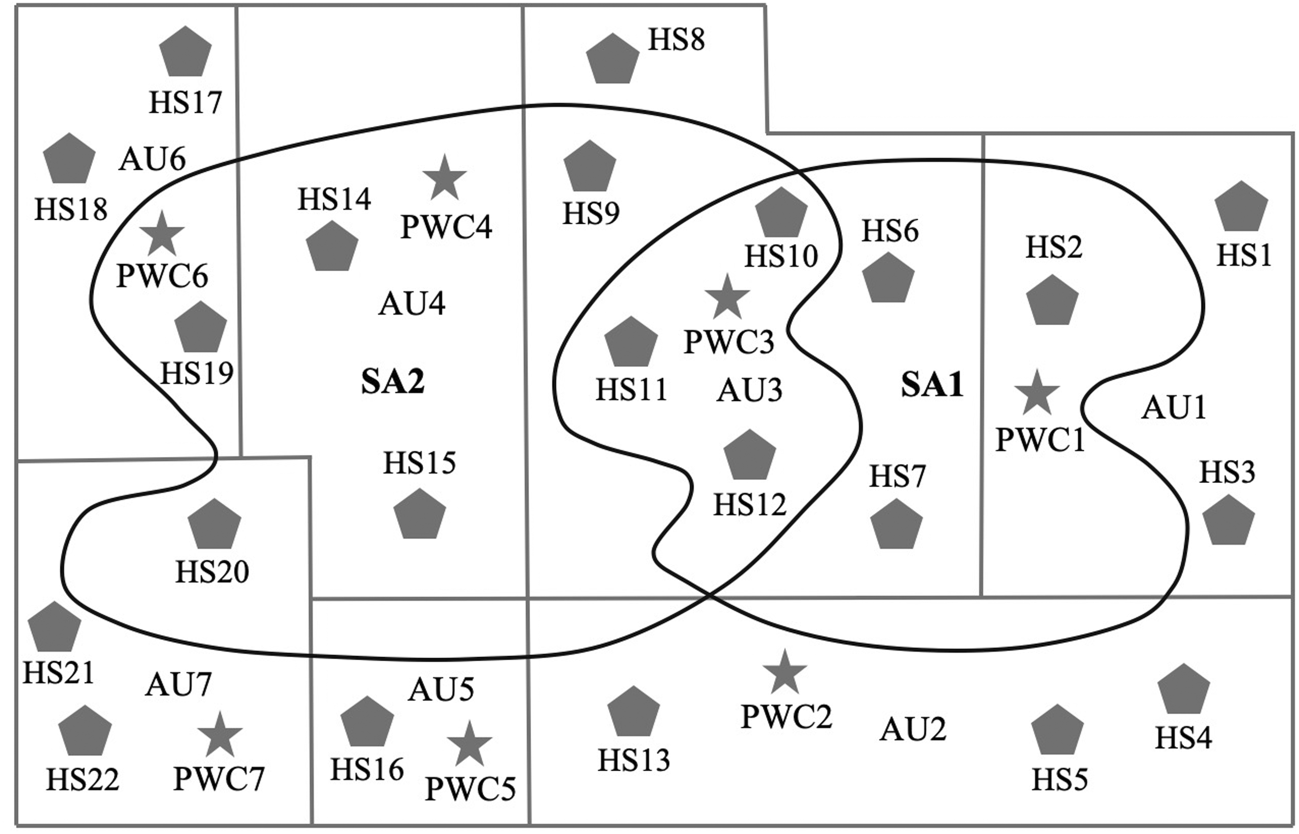
The conceptual diagram of how to take into account the overlay of SAs in PAB measurement applying the HSW and PWC techniques.

As can be seen from Figure 1, when applying the HSW technique, the weight of ‘1/3’ is assigned to AU1, AU6 and AU7 each as one out of the three HSs within each of the three AUs is located inside SA1 or SA2. The weight of ‘0’ is assigned to AU2 and AU5 each as all HSs within them (three and one respectively) are located outside both SA1 and SA2. The weight of ‘1’ is assigned to AU4 as all its HSs (two) are located inside SA2. AU3 has HSs (HS10–12) located inside both SA1 and SA2. A weight of ‘5/7’ is assigned to AU3 as five out of its seven HSs are located inside SA1; another weight of ‘4/7’ is assigned to it as four out of its seven HSs are located inside SA2. Thus, the weight of ‘9/7’ (‘5/7 + 4/7’) is assigned to AU3 in total applying the HSW technique.

When applying the PWC technique, the weight of ‘1’ is assigned to AU1 as its PWC is located inside SA1. The weight of ‘1’ is assigned to AU4 and AU6 each as their PWCs are located inside SA2. The weight of ‘0’ is assigned to AU2, AU5 and AU7 each as their PWCs are located outside both SA1 and SA2. The PWC of CU3 is located inside the overlay of SA1 and SA2. A weight of ‘1’ is assigned to AU3 as its PWC is located inside SA1; another weight of ‘1’ is assigned to AU3 as its PWC is located inside SA2. Thus, the weight of ‘2’ is assigned to AU3 in total applying the PWC technique.

The fundamental difference between the HSW and PWC techniques lies in their different ways of assigning weights to AUs with access. The PWC technique assigns the weight of ‘1’ to an AU so long as its PWC located inside the SA, while the HSW technique only assigns the weight of ‘1’ to an AU with all its HSs located inside the SA. That’s why there are underestimations (e.g. AU7) and overestimations (e.g. AU1,3,6) of the population located inside the SA when applying the PWC technique compared to the HSW technique.

The way in which the PWC technique assigns the weight to the AU with access and the resultant underestimations and overestimations are the source of aggregation errors. When the weight of ‘0’ is assigned to an AU with its PWC located outside the SA, it assumes that no population within the AU is located inside the SA. When the weight of ‘1’ is assigned to an AU with its PWC located inside the SA, it assumes that the whole population within the AU is located inside the SA. However, this does not reflect reality. In contrast, the HSW technique assigns the weight to an AU with access based on the proportion of its HSs located inside the SA. Apart from the weight of ‘0’ or ‘1’, the HSW technique assigns the weight of ‘0–1’ to an AU with parts of its HSs located inside the SA, that is partial access.

Thus, conceptually, the HSW technique is more accurate than the PWC technique in estimating population inside SAs by assigning weights to AUs in a more accurate way. Consequently, the HSW technique is more accurate in calculating PAB for social groups, as the calculation is carried out by multiplying the weight of each AU with access by the number of each social group within the AU. The impact of this conceptual difference on PAB and PA measurement in practice at the city scale will be explored within a case study of GP practices in Newcastle.

Case study

Newcastle is located in the North East of England, UK, with 910 output areas (OAs) within its administrative boundary. The city has a population of 280,177; there are 117,153 households, of which 69,649 (59.45%) are deprived and 47,504 (40.55%) are non-deprived households according to the 2011 Census Data (ONS, 2017).

The purpose of the case study is to provide an illustration of the application of the PWC and HSW techniques to estimate population inside SAs and measure PAB and PA to GP practices for social groups (i.e. the deprived and non-deprived households) at the city scale. The case study will use the lowest level census data available in the UK, i.e. the OA level. But the use of both the National Statistics of Postcode Lookup Centroid (NSPLC) and the population weighted centroid of the output area (OAPWC) will be compared to that of the HS. Related comparisons will be made in the Discussions section.

Data preparation

In order to illustrate the application of the HSW and PWC techniques and compare them in the PAB and PA measurement for the deprived and non-deprived households in Newcastle, the following datasets were prepared: (1) GP practices (44 in total updated according to GP data, NHS GP practice online search data and GP practice websites as at September 2017); (2) the 2011 Census Data deprivation dataset; (3) HSs; (4) 2011 OAPWCs; (5) NSPLCs; (6) Ordnance Survey ITN road and footpath networks; (7) OA boundaries; and (8) Newcastle boundary.

Here, network distance, rather than straight line distance, is used to create SAs, because the former is closer to reality, as most people use roads and/or footpath networks to reach services (Christie and Fone, 2003). Walking is the travel mode used within the analysis because the disadvantaged social group maybe less likely to own a car and may even have difficulties in affording public transport. Half a mile is selected as the maximum walking distance threshold because this is often regarded as the ceiling for walkers of disadvantaged social groups (Hillman et al., 1973).

The application and comparison of the PWC and HSW techniques in the PAB and PA measurement for social groups in Newcastle at the city scale

The percentages of PAB and PA were calculated for the deprived and non-deprived households in Newcastle taking into account the overlay of SAs applying the HSW and PWC techniques based on the illustration in the Section ‘A conceptual comparison between the HSW and PWC techniques’. For the HSW technique, residential buildings in Newcastle by dwelling type in use that take into account houses in multiple occupancy were selected by cleansing the AddressBase Premium data ⁴ provided by Ordnance Survey and the UKBuildings data ⁵ purchased from GeoInformation Group. This is key to disaggregating census data from the lowest available AU level (i.e. the OA level in this case) to the household level and then calculating the number of HSs to represent the number of households for each AU.

The 118,086 buildings selected in the data cleansing process are residential buildings in use reflecting dwelling types and taking into account houses in multiple occupancy in Newcastle. Thus, the ‘multiple occupancy count’ (using the ‘MULTI_OCC’ dataset) of each of the 118,086 residential buildings plus ‘1’ equals to the number of HSs in the corresponding residential building. The equations illustrated in the subsection ‘Introduction to the four-step HSW technique’ were then used for the calculations.

For the PWC technique, the PWCs of the 910 OAs were downloaded from the ONS website (ONS, 2013). Identifying PWCs that are located inside SAs is key to the calculations. This is achieved by identifying the relationship between the location of PWCs and SAs. Table 1 shows different results of the numbers and percentages of the deprived and non-deprived households with PAB and PA to GP practices in Newcastle at the city scale applying the HSW and PWC techniques.

Table 1.

The difference in numbers and percentages of social groups with PAB and PA to GP practices in Newcastle at the city scale applying the two techniques.

Variable	Technique	No. of PAB	Total no. of social group/OA involved in PAB calculations	% of PAB	% of PA
Deprived household	HSW	50,643	97,670/1282	51.85	1.2441
	PWC	50,442	82,440/1078	61.19	1.4705
Difference		–201		9.34	18.2a
Non-deprived household	HSW	34,607	69,296/1282	49.94	1.2216
	PWC	34,732	57,932/1078	59.95	1.4646
Difference		125		10.01	19.89a

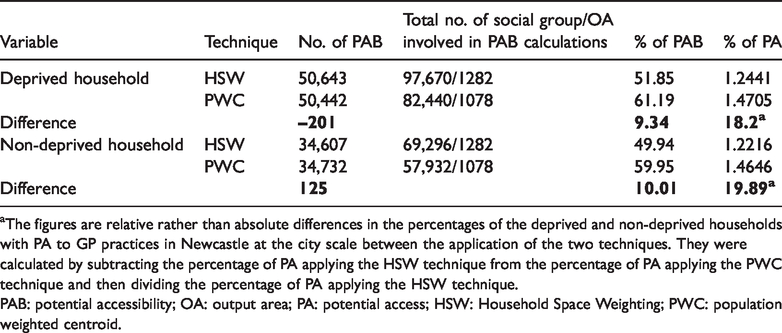
^aThe figures are relative rather than absolute differences in the percentages of the deprived and non-deprived households with PA to GP practices in Newcastle at the city scale between the application of the two techniques. They were calculated by subtracting the percentage of PA applying the HSW technique from the percentage of PA applying the PWC technique and then dividing the percentage of PA applying the HSW technique.

PAB: potential accessibility; OA: output area; PA: potential access; HSW: Household Space Weighting; PWC: population weighted centroid.

It is worth noting here that the number of OAs involved in the calculation of the total number of each social group with PAB at the city scale exceeds the total number of OAs (910) in the city applying both HSW and PWC techniques (1282 and 1078 OAs respectively). This is because there are overlaid SAs involved in the calculations at the city scale (explained earlier in the Section ‘A conceptual comparison between the HSW and PWC techniques’). Accordingly, the total numbers of the deprived household (97,670 and 82,440 respectively) and the non-deprived household (69,296 and 57,932 respectively) involved in the calculations applying the HSW and PWC techniques exceed the total numbers of the deprived household (69,649) and the non-deprived household (47,504) respectively in the city.

Discussions

Empirical comparison between the use of NSPLCs or PWCs and HSs in population estimates and related aggregation errors

This subsection will use empirical data to further explain the difference between the use of NSPLCs or PWCs and HSs in population estimates and related aggregation errors caused by using NSPLCs and PWCs. A SA of a random GP practice in the city was selected (see Figure 2(a) and (b)) to visualize such differences and related aggregation errors.

Figure 2.

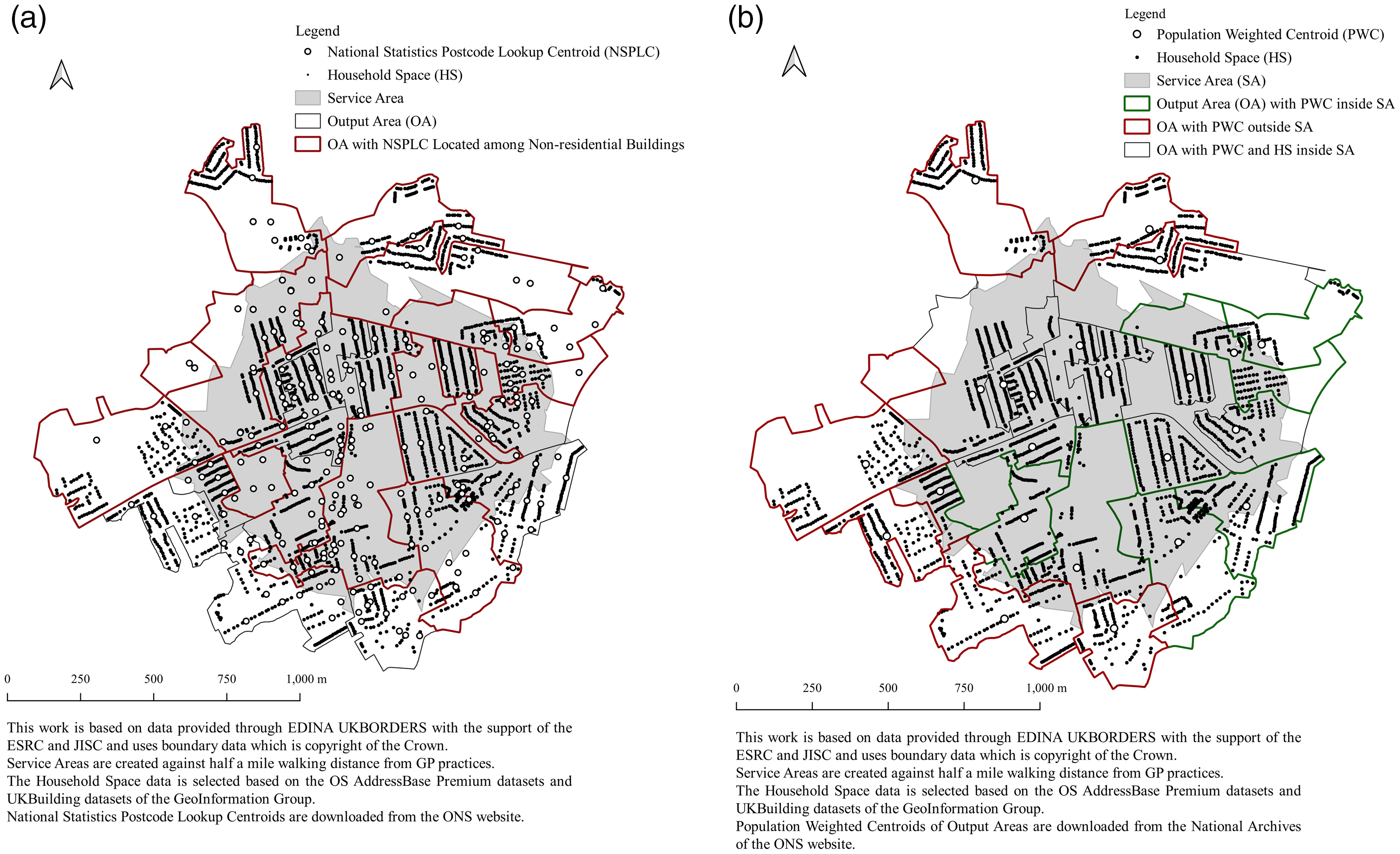
Visualization of aggregation errors.

Figure 2(a) visualizes aggregation errors by comparing the use of NSPLCs and HSs. Even though the majority of NSPLCs within OAs in black are located among residential buildings, there are NSPLCs within OAs (in red) located among non-residential buildings which cannot represent the location of populations. Thus, aggregation errors occur when NSPLCs are used to provide population estimates inside the SA. For the whole city, when the proportion of NSPLCs within each OA located inside the SA is used to provide population estimates inside the SA (i.e. the NSPLC technique), it produces inaccurate population estimates for 402 (233 underestimations and 169 overestimations) out of the 910 OAs (44%) in Newcastle.

Figure 2(b) visualizes aggregation errors by comparing the use of PWCs and HSs. There are OAs (in black) with their PWCs and all HSs located inside the SA applying both the PWC and HSW techniques. However, there are OAs (in green) with their PWCs located inside the SA when applying the PWC technique while only partial HSs within those OAs are located inside the SA when applying the HSW technique. There are OAs (in red) with their PWCs located outside the SA when applying the PWC technique, whereas partial HSs within those OAs are located inside the SA when applying the HSW technique. For the whole city, the PWC technique produces inaccurate population estimates for 267 (131 underestimations and 136 overestimations) out of the 910 OAs (29%) in Newcastle.

As can be seen by comparing Figure 2(a) and (b) that there are more centroids in each OA using NSPLCs than PWCs, but the PWC technique produces less inaccurate population estimates inside the SA because the median centroid algorithm used in the calculation of PWCs takes into account the location of households (ONS, 2013). However, the dichotomous categorization of OAs in population estimates applying the PWC technique does not reflect reality and is the source of aggregation errors as illustrated earlier.

On the other hand, the HSW technique takes into consideration all three categories, i.e. OAs with the whole, partial or no population located inside the SA. By identifying the location of HSs to represent households, the HSW technique reduces aggregation errors. The level of aggregation errors using less accurate techniques depends, to some extent, on the type of residential buildings, i.e. higher level of aggregation errors may occur to AUs with more high rises than houses as, in general, the former accommodate more households than the latter.

Empirical comparison between the PA measurement results applying the HSW and PWC techniques

This subsection will focus on comparing the PA measurement results applying the two techniques. The results calculated in the Case Study section (see Table 1) indicate that the difference is small in the number of each social group with PAB to GP practices between the application of the two techniques at Newcastle city scale. This means that even though there are underestimations and overestimations of the populations inside SAs when applying the PWC technique, they are evened out when the scale of analysis is the whole city rather than each SA within the city.

However, the difference in the percentage of social groups with PAB or PA between the application of the two techniques is large. As shown in Table 1, there are considerable differences in the percentage of the deprived household and the non-deprived household with PAB and PA to GP practices in Newcastle at the city scale, respectively, between the application of the two techniques. When calculating the denominators so as to calculate the percentages of social groups with access, the PWC technique does not take into account the OAs with their PWCs located outside SAs while with partial population located inside the SAs. Thus, there are fewer OAs involved in the calculation of the denominators applying the PWC technique (1078 OAs) compared to the HSW technique (1282 OAs). As such, the denominator of each social group involved in the calculations is smaller when applying the PWC technique. Given that the differences in the numerator of each social group involved in the calculations between the application of the two techniques are relatively small at the city scale, the percentages of each social group with PAB and PA applying the PWC technique are higher than applying the HSW technique, respectively, at the city scale.

Therefore, even though the difference in the number of each social group with PAB is small, the differences in the percentage of each social group with PAB and PA are large, respectively, at the city scale. The absolute difference in the percentage of PAB is 9–10% and the relative difference in the percentage of PA is 18–20% between the application of the two techniques (see Table 1). The large difference in the percentage is important because it is the percentage rather than the number of each social group with PAB or PA that is comparable due to different population size of each social group in a city. For policy implications, the large difference suggests that if service planners or policy makers want to measure PAB or PA of social groups to services for cities, it would be useful to apply a more accurate technique, or at least be aware of the implications of applying the PWC technique.

Conclusions

The research reviewed the existing studies on the ‘ecological fallacy’, MAUP, aggregation error issue, population estimates inside SAs and PAB and PA measurement. The prevalence of place access rather than population access in the existing studies due to the unavailability of household-level census data causes the aggregation error issue. To reduce aggregation errors, there are spatial disaggregation techniques (e.g. dasymetric mapping) which intend to identify the location of populations by locating residential buildings and other techniques which intend to improve spatial representation of AUs (e.g. the use of PWCs to replace GCs to represent AUs). However, aggregation errors still occur when using these techniques to measure PAB and PA.

This research has shown that even though the use of PWCs provides less inaccurate population estimates inside the SA than using NSPLCs, the dichotomous categorization of OAs in population estimates applying the PWC technique does not reflect reality and is the source of aggregation errors. Drawing upon Maantay et al.’s (2007) and Luo and Wang’s (2003) studies, this research develops a more accurate population weighting technique – the HSW technique. The technique uses the most up-to-date and accurate cadastral and address-based data to reduce aggregation errors by disaggregating census data from the lowest available AU level to the household level.

The conceptual comparison has demonstrated that the HSW technique is more accurate than the PWC technique in population estimates inside the SA. Instead of assigning the weight of either ‘0’ or ‘1’ to an AU (i.e. no access or full access) when applying the PWC technique, the HSW technique assigns the weight of ‘0’, ‘0–1’ or ‘1’ to an AU (i.e. no access, partial access or full access). The HSW technique is closer to reality because it is unlikely that populations within the AU are located either fully inside or outside the SA. Rather, they are located fully or partially inside or outside the SA due to the uneven distribution of the populations and the heterogeneity of the physical environment within the AU (Crawford, 2006; Hewko et al., 2002; Knox, 1979). The empirical comparison has tested this, which shows that the PWC technique produces inaccurate population estimates for 267 out of the 910 OAs (29%) in Newcastle.

The research has also demonstrated that the HSW technique is more accurate than the PWC technique in measuring PAB and PA at the city scale. The difference in the percentage of social groups with PAB or PA to GP practices at the city scale is considerable, with the absolute difference in the percentage of each social group with PAB of 9–10% and the relative difference in the percentage of each social group with PA of 18–20% between the application of the two techniques. The large difference in the percentage is important because it is the percentage rather than the number of each social group with PAB or PA that is comparable due to different population size of each social group in a city. Such difference suggests that if service planners or policy makers wish to measure PAB or PA of social groups to services for cities, they should ideally use a more accurate technique, or at least be aware of the implications of applying the PWC technique.

This research contributes to better estimating population inside SAs and measuring PAB and PA to services in a generic way for social groups at the city scale. In the absence of household-level census data, the HSW technique can be used to disaggregate census data from the lowest available AU level to the household level. The HSW technique can also be used as a population access measurement method to assess PA to services for social groups and provide policy recommendations based on the comparison between the advantaged and disadvantaged social groups with PA at the city scale.

For decades, researchers have investigated issues related to the ‘ecological fallacy’, MAUP and aggregation errors (Jelinski and Wu, 1996; Jones et al., 2018; Openshaw, 1984; Openshaw and Taylor 1979; Robinson, 2009) and strived to improve the accuracy of population estimates and PAB and PA measurement by further disaggregating census data from the lowest available AU level and/or by improving spatial representation of AUs. This paper has explored further minimization of aggregation errors and better measurement of PAB and PA to services for social groups at the city scale by introducing the HSW technique. For future research, it would be worth applying the HSW technique to measure PA to services for social groups in other cities where household-level census data are not available. It would also be worth applying the HSW technique to compare the level of PA to that of the utilization of services for social groups at the city scale.