Sage Journals: Discover world-class research

Abstract

Level-of-service has been widely used to measure the operational efficiency of existing highway systems categorically, based on certain ranges of traffic speeds. However, this existing method is generic for investigating urban traffic characteristics. Hence, there is a crucial knowledge gap in capturing the unique traffic speed conditions during a certain temporal duration, in a common spatial area that includes different land use clusters. This study fills this gap by modeling the link between traffic speeds and land use clusters during certain time periods, along with the given level-of-service criteria. As a case study, this study adopted the central business district in Los Angeles in the United States. A total of 1780 traffic sensor speed data on Interstate 10 East adjacent to the central business district of Los Angeles was collected and clustered by the land use designated by the zoning regulations of the city of Los Angeles. The proposed traffic time–speed curve model that integrates different land uses in a large urban core was then developed and validated statistically, using historical real-world traffic data. Finally, an illustrative example was presented to demonstrate how the proposed model can be implemented to measure critical time periods and corresponding speeds per land-use cluster, responding to the designated level-of-service criteria. This study focused on making recommendations for government transportation agencies to employ an appropriate method that can estimate critical time periods affecting the existing operational status of a highway segment in different land-use clusters within a common spatial area, while promoting an effective application of a set of traffic sensor speed data.

Keywords

Level-of-service land use central business district traffic congestion time–speed

Introduction

Most urban areas include typical land use types such as businesses, residential areas, attractions, and remote areas, each having their own unique socioeconomic and demographic characteristics. An essential component that interacts with these typical land use clusters is road networks (Chaudhuri and Clarke, 2015). Spatially, road networks play a key role in measuring, characterizing, and assessing the demand for transportation associated with urban characteristics and each of the land-use types (Chaudhuri and Clarke, 2015; Harding et al., 2014; Lowry and Balling, 2009). In large urban areas, central business districts (CBDs) are defined as a key urban structure type (i.e. the urban core), which commonly appear throughout large cities because of numerous economic activities (Taubenböck et al., 2013). Nilsson and Smirnov (2016) found that economic activities in CBDs are significantly affected by changes in the transportation system, such as the potential capacity expansion and the proximity to transportation infrastructure.

Given the strong interaction between land use clusters and road infrastructure, traffic congestion negatively affects productivity and the costs to society, while wasting time and energy (Rao and Rao, 2012). The impact of inconvenience appears in the form of travel time increases, queue delays, reduction of highway capacity, potential increase of accident rates, and a higher level of the traveling public’s dissatisfaction (Karim and Adeli, 2003; Rao and Rao, 2012; Zhu et al., 2009). In general, severe traffic congestion is often shown in heavily trafficked urban areas (Zhu et al., 2009), resulting in the average driver burning 67 hours and 32 extra gallons of fuel each year in the United States (Hasley, 2013). To overcome these obstacles, it is believed that identifying and characterizing traffic congestion is the first step to mitigating congestion, depending on the urban characteristics and the corresponding land use clusters (Rao and Rao, 2012).

Level-of-service: A congestion measurement method

Congestion measurement methods should be clearly comprehensible, applicable to statistical techniques, and replicable based on the results with a minimum amount of data collected during certain time periods (Rao and Rao, 2012). In this regard, level-of-service (LOS) is one of the most widely-used congestion measurement methods, specifically aimed at measuring traffic congestion and assessing the operational efficiency of existing road networks (Bhuyan and Nayak, 2013; Das and Pandit, 2016; Dowling et al., 2008; Ghods and Saccomanno, 2016; Jolovic et al., 2016; Ramadan and Sisiopiku, 2016; Rao and Rao, 2012).

As a qualitative measure, LOS allows non-technical audiences to capture the level of traffic flows easily (Rao and Rao, 2012). LOS measures and describes the operational effectiveness of a roadway segment with letter designations A through F (Alameda County Transportation Commission, 2012; Bhuyan and Nayak, 2013). LOS A is the best performing service, which indicates a free flow of traffic with little or no delay. On the other hand, LOS F is the worst service, accompanied by traffic flows exceeding the capacity, thereby resulting in long queues and delays (Transportation Research Board, 2010). Specifically, the Highway Capacity Manual (HCM) in the United States provides the list of six different ratings of LOS (Transportation Research Board, 2010):

A: Free flow operations at average travel speeds

B: Reasonably unimpeded operations by maintaining LOS A

C: Stable flow, but restricted to maneuver through lanes

D: Approaching unstable flow with decreasing speeds as traffic volume slightly increases

E: Unstable flow operations at capacity

F: Arterial flow at extremely low speeds

The assessment of facility performance as described in the HCM is dependent on each different type of roadway segment (e.g. mainline, weave, merge, diverge) (Jolovic et al., 2016). The HCM procedures have constraints on achieving realistic and reliable data, which are a key factor for evaluating the operating status of roadway segments.

Point of departure: Knowledge gaps

Employing quality data

To overcome the limitation of HCM procedures on a LOS analysis, FREEVAL was developed in Microsoft Excel with Visual Basic Applications, which is a supplementary computational engine associated with the HCM. FREEVAL is a deterministic equation-based macroscopic and mesoscopic tool that provides segment-based densities to evaluate freeway facilities (Jolovic et al., 2016; Transportation Research Board, 2010). Jolovic and Stevanovic (2012) have pointed out that FREEVAL is incapable of capturing actual field data, such as speed and density under oversaturated freeway conditions.

Compared to deterministic equation-based methods, most of the traffic simulators developed in recent decades adopt microscopic simulation models (Ben-Akiva et al., 1998; Ermagun and Levinson, 2019; Hourdakis et al., 2003; Kamarianakis and Prastacos, 2005). Previous research efforts on coupling spatial areas and road networks have also been made, based on simulation models (Anderson et al., 1996; Chaudhuri and Clarke, 2015; Ermagun and Levinson, 2019; Kanaroglou, 1999; Pendyala et al., 2012; Strauch et al., 2005; Waddell, 2002). However, these simulation methods demonstrate a critical limitation as they cannot capture global descriptions of the traffic flow-rate, density, and velocity and are often restricted to synthetic or simplified data (Van Lint et al., 2002).

Therefore, many previous studies have not reflected real-world situations in the modeling process, due to a lack of quality data. Data quality is defined based on various dimensions, such as accuracy, objectivity, credibility, accessibility, amount of data, and consistency (Strong et al., 1997; Wang et al., 1995). In the context of quality data in traffic domains, for example, the Performance Measurement System (PeMS) is a very well-known archived data user service operated by the California Department of Transportation (Caltrans, 2019). PeMS converts freeway sensor data into intuitive tables and graphs that show historical and real-time traffic measurements, by collecting traffic data every 30 seconds from over 15,000 individual loop detectors that are placed in California freeways (Bae et al., 2017; Chen et al., 2001; Lv et al., 2015). Nevertheless, even if high quality data are available, as archived traffic measurements read by a number of sensor devices at different locations within a common spatial area are different from each other, engineers in government transportation agencies and urban planners find it difficult to promote an effective application of a set of real-world historical traffic speed data to establish an effective strategy or policy that can reduce traffic congestion.

Linking land use clusters to critical time–speed estimation

The significance of coupling between land use and transportation planning or modeling has been highlighted by previous studies (Chaudhuri and Clarke, 2015; Handy, 2005; Hunt and Simmonds, 1993; Lowry and Balling, 2009; Maat et al., 2005). In recent years, Chaudhuri and Clarke (2015) provided a thorough review of previous studies on quantitative approaches to the integration between land use and road networks on the macroscopic level. In addition, Lowry and Balling (2009) presented a new approach to land use and transportation for both city and region planning stages, called district land-use scenarios. In turn, the scope of most previous studies is broad so that it is insufficient to capture the unique characteristics of highway congestion in each different land use cluster within a common spatial area.

When considering that most urban areas include highway segments within a particular spatial area that is characterized by different land use clusters, such as commercial, industrial, residential, and areas of attraction, existing methods are incapable of capturing the unique characteristics of LOS in a particular land use cluster. Given the spatial variability, there is very little known about appropriate methods that can estimate critical time periods affecting the existing operational status of a highway segment in different land use clusters within a common spatial area.

Research objectives and methods

As stated above, most existing studies have explored LOS of roadway systems through simulation methods, which often do not reflect real-world situations within a certain spatial area (e.g. urban downtown areas) accurately. In addition, the scope of analysis zones conducted in previous studies is too broad to capture the unique characteristics of traffic patterns in each different land use cluster within a common spatial area. This study fills these gaps by modeling the link between traffic speeds and land use clusters during certain time periods, in line with the given LOS criteria. Considering the impact of highway traffic on large urban cores, the main objectives of this study are to develop and validate a traffic time–speed curve model, specifically aiming at assessing critical time periods and the corresponding traffic speeds in different land use clusters within a common spatial area, as depicted in Figure 1.

Figure 1.

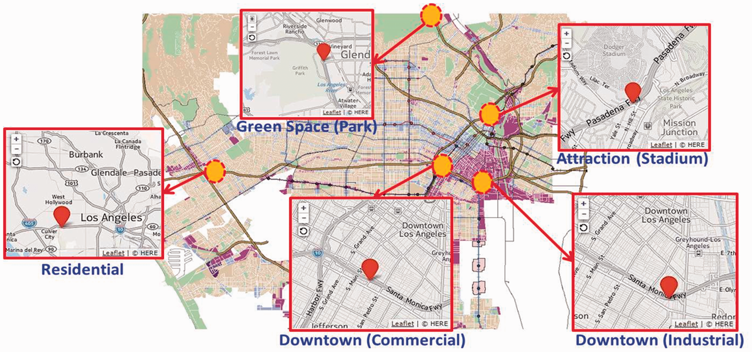
Typical spatial areas along with large urban corridors.

To this end, as a case study, this study adopted the CBD in Los Angeles (LA) in the United States. The State of California (2001) classifies land use clusters into both general locations and the intensity of housing, business, industry, open space, education, public buildings and grounds, waste disposal facilities, and others. In line with the existing designation, the CBD in LA includes predominantly commercial and industrial land use elements. Accordingly, land use clusters considered in this study are drawn as location and intensity-based classification. The objective of this study was achieved through the following six-stage methodology:

A total of 1780 traffic speed measurements were collected from traffic sensors located on Interstate 10 East (I-10 E) highway adjacent to the CBD of LA (hereafter “Downtown LA”), which were extracted from the Caltrans PeMS (Caltrans, 2019).

Along I-10 E, traffic sensors on the highway were clustered by mapping with the corresponding land uses that are designated by zoning regulations of the City of LA, using ArcGIS (Department of City Planning-City of Los Angeles, 2006).

A hypothesis test was conducted using the Kruskal–Wallis test and the Wilcoxon test methods to scientifically examine whether there is a significant difference in average travel speed measurements on the highway network near two different land use clusters in Downtown LA (i.e. commercial and industrial land uses) and how they are different from each other.

A time–speed model for the land use clusters was then developed through a fourth-order (i.e. quartic) polynomial regression analysis.

The robustness of the developed model was validated by one of the most widely-used cross-validation methods, the Predicted Residual Error Sum of Squares (PRESS) statistic (Ott and Longnecker, 2010).

An illustrative example was then presented to demonstrate how the proposed model can be implemented practically to measure LOS adjacent to the studied large urban core that includes commercial and industrial land use clusters.

The following are assumptions and limitations of this study:

It was assumed that traffic speed patterns during the studied time period are very similar with historical traffic patterns over entire years.

It was assumed that average travel speed data sets extracted from the traffic sensors numerically represent the existing road facility information (e.g. number of lanes, entrances/exits, interchanges/junctions) and geographical conditions (e.g. location, the proximity to land uses) that affect the operational efficiency of I-10 E near the studied land use clusters.

It was assumed that traffic patterns on I-10 West are symmetric with those on I-10 E.

This study assumes that neither an incident nor an accident occurs.

The scope of the highway network examined is limited to mainline in multi-lane unidirectional highways, excluding ramps, intersections, and HOV lanes.

Traffic sensor data collected in this study are confined to average travel speed measurements during typical weekdays (i.e. Monday to Friday), excluding speed data during weekends and holidays.

Data collection and classification

As depicted in Figure 2(a), I-10 E adjacent to Downtown LA was selected as the traffic analysis network to gather traffic sensor speed data that can be benchmarked with other large urban cores. LA has long been one of the most trafficked metropolitan areas in the United States (TRIP, 2014). More specifically, I-10 near Downtown LA ranks third on the list of the most congested highways in the nation (Romero, 2015).

Figure 2.

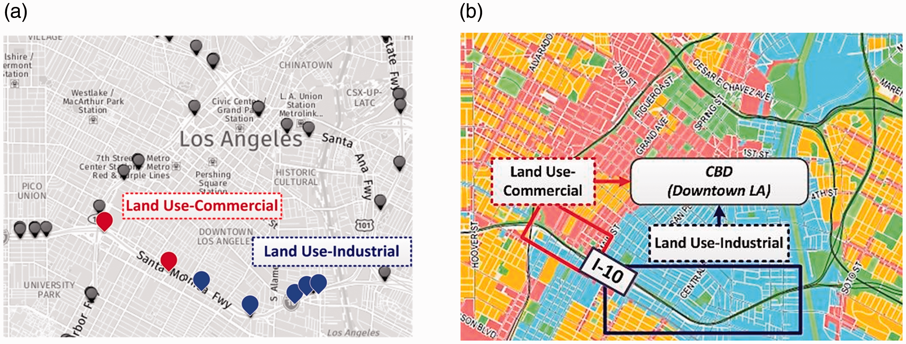
Traffic analysis zone: Downtown LA along I-10 E.

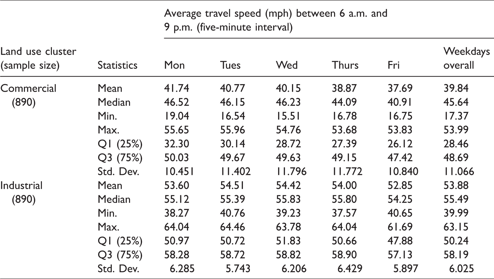
Along with the highway network, a total of 1780 traffic sensor measurements (i.e. average travel speed) on I-10 E was randomly collected between 6:00 a.m. and 9:00 p.m. during weekdays in the first quarter of the year 2016, using the Caltrans PeMS (see Figure 2(a)) (Caltrans, 2019). More specifically, traffic speed data sets were extracted from PeMS, over a five-minute interval during the collection time period per day (i.e. Monday to Friday). Meanwhile, using ArcGIS, the common spatial area (i.e. Downtown LA) was grouped by commercial and industrial land uses that are designated by the zoning regulations of the City of LA, as seen in Figure 2(b) (Department of City Planning-City of Los Angeles, 2006). Subsequently, the averaged traffic speed data sets were mapped with the corresponding land use clusters and then averaged on a daily basis, considering different numbers of traffic sensor locations available on the highway network (see Figure 2(a)). In turn, a total of 890 sensor measurements were used to represent each land use cluster (i.e. 1780 = 890 × 2 land uses). Table 1 summarizes the average travel speed data sets in the two different land uses on daily basis and during weekdays.

Table 1.

Descriptive statistics of the average travel speed data sets.

Land use cluster (sample size)	Statistics	Average travel speed (mph) between 6 a.m. and 9 p.m. (five-minute interval)
Land use cluster (sample size)	Statistics	Mon	Tues	Wed	Thurs	Fri	Weekdays overall
Commercial (890)	Mean	41.74	40.77	40.15	38.87	37.69	39.84
	Median	46.52	46.15	46.23	44.09	40.91	45.64
	Min.	19.04	16.54	15.51	16.78	16.75	17.37
	Max.	55.65	55.96	54.76	53.68	53.83	53.99
	Q1 (25%)	32.30	30.14	28.72	27.39	26.12	28.46
	Q3 (75%)	50.03	49.67	49.63	49.15	47.42	48.69
	Std. Dev.	10.451	11.402	11.796	11.772	10.840	11.066
Industrial (890)	Mean	53.60	54.51	54.42	54.00	52.85	53.88
	Median	55.12	55.39	55.83	55.80	54.25	55.49
	Min.	38.27	40.76	39.23	37.57	40.65	39.99
	Max.	64.04	64.46	63.78	64.04	61.69	63.15
	Q1 (25%)	50.97	50.72	51.83	50.66	47.88	50.24
	Q3 (75%)	58.28	58.72	58.82	58.90	57.13	58.19
	Std. Dev.	6.285	5.743	6.206	6.429	5.897	6.025

Initial data analysis: Average travel speed versus land use

In general, statistical analysis of the data in transportation problems violates the assumption of the normality of the data (Spiegelman et al., 2011). A lack of normality in ANOVA causes leads to significant inflation of the error sum of squares due to outliers. To overcome this difficulty, the Kruskal–Wallis approach to ANOVA was conducted, which compares the medians of two or more samples. As a nonparametric alternative, this distribution-free test is robust to the existence of outliers in which the raw data are replaced with ranked data (Ott and Longnecker, 2010; Spiegelman et al., 2011).

Since the distribution of traffic speed data proves to be non-normal (Figure 3(a)) and the variances clustered by commercial and industrial land uses in Downtown LA are different as shown in Figure 3(b), the Kruskal–Wallis approach is available to compare the clustering groups.

Figure 3.

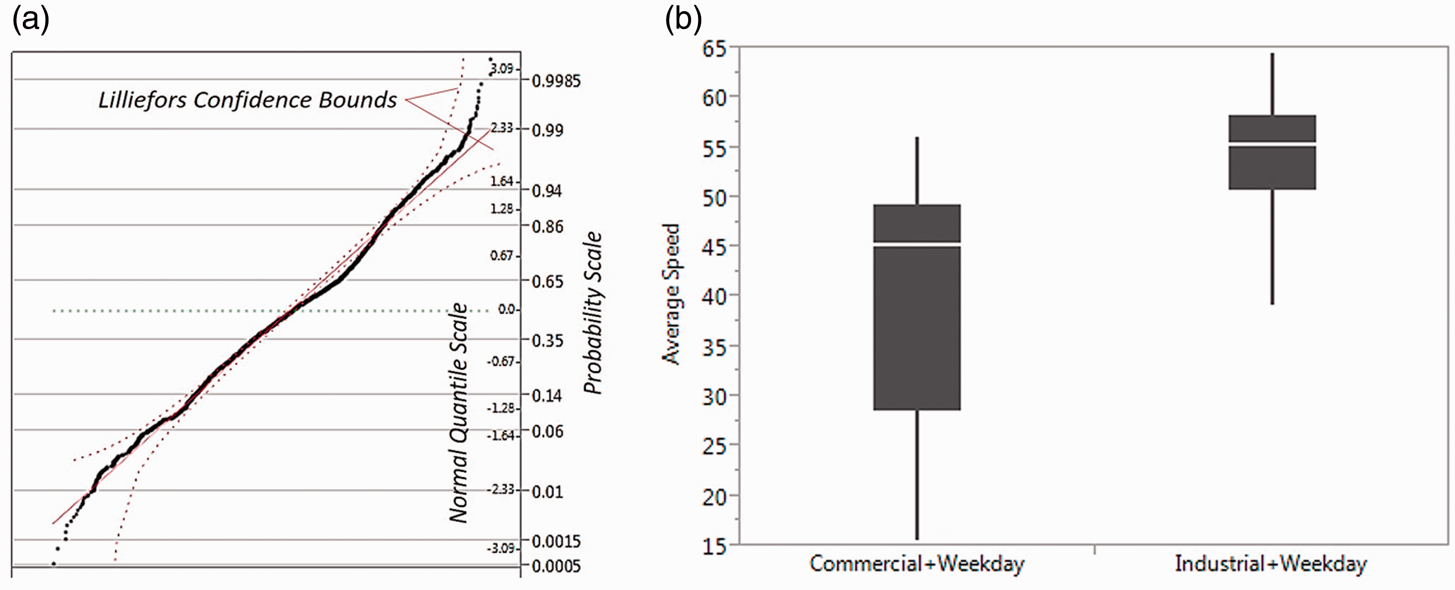
Initial data investigation. (a) Violation of the normality assumption; (b) Comparison of average speed data between commercial and industrial land uses.

The following hypothesis is established to test the difference between two land use clusters:

H₀: There is no statistically significant difference in average traffic speeds in commercial and industrial land uses within a common spatial area.

H_a: There is a statistically significant difference in average traffic speed measurements in different land uses within the common spatial area.

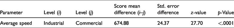
The test results confirmed that I-10 E average travel speed data samples come from a different population by having a high chi-square value of 767.2085 and p-value much less than .0001. To scientifically test the established hypothesis further, the Wilcoxon matched-pairs signed ranks test was conducted to examine whether the result of one measure is significantly different from the other through matched-pairs signed ranks. The following hypothesis was established to test whether vehicle speeds under two different land use clusters are different from each other, at the significance level (α) of 0.05:

The industrial land use cluster in Downtown LA would result in higher speed during weekdays, compared to the speed in the commercial land use cluster.

The test result as seen in Table 2 revealed that traffic congestion near the commercial use in Downtown LA (j) is much heavier than the industrial use (i), with a p-value less than .0001.

Table 2.

Wilcoxon test results of nonparametric comparisons for each pair.

Parameter	Level (i)	Level (j)	Score mean difference (i–j)	Std. error difference	z-value	p-Value
Average speed	Industrial	Commercial	674.88	24.37	27.70	<.0001

Modeling the link between highway traffic speed and land use

Designing a quartic polynomial regression model

The validity of the regression model is determined based on certain assumptions of the normality, homogeneity of variances, and homoscedasticity. The validation of these assumptions is essential for a reliable interpretation of causal relationships among the variables in the model (Jafarzadeh et al., 2013).

Given that this study uses non-normally distributed data for the analysis, there is a high possibility of heteroscedasticity. The existence of heteroscedasticity is a major concern when conducting a regression analysis because it can cause biased results. To tackle this issue, the proposed time–speed model was transformed to a fourth-order (quartic) polynomial regression form after comparing the fitted lines of a number of different transformed models. In addition, the dependent variable of speed was transformed to a squared form, to improve the accuracy and reliability of the proposed statistical model. A categorical variable was incorporated into the model in order to determine how traffic speed patterns for the two land use clusters are statistically different from each other as outlined below:

Transformed Speed = {(Speed)}^{2} = β_{0} + β_{1} Time + β_{2} {Time}^{2} + β_{3} {Time}^{3} + β_{4} {Time}^{4} + β_{5} I_{1}

(1)

where

Speed: Average traffic speed (mph)

Time: 24-hour time designation as continuous values (e.g. 1: 15 p.m. = 13.25)

I: Indicator, if I₁ = 1: Commercial land use

if I₁ = ‒1: Industrial land use

As shown in equation (1), the indicator of a categorical variable in the regression model was numerically represented using an effect coding method that takes values of –1, 0, and 1 for the categorical variables. The effective coding has a benefit that both the main effects and interaction can be reasonably estimated, compared to other commonly used method of dummy coding. The dummy coding focuses on showing the interaction of groups by taking 0 and 1 for the categorical variables, not the main effect itself (Choi et al., 2015b; Cornell University, 2008).

In the application of a regression analysis, it is assumed that the standardized residuals should be normally distributed as the null hypothesis. A normal quartile–quartile (Q–Q) plot of the standardized residuals displays approximately normally distributed data, as shown in Figure 4(a). In the proposed model, the mean and standard deviation of these residuals were calculated to be .01 and .94, respectively. These values are almost the same as those used to describe a standard normal distribution (i.e. mean: 0 and standard deviation: 1). To scientifically test the normality, Fisher’s exact test was performed by comparing the mean standard deviation values obtained from the proposed model with those in the standard normal distribution. The two-sided test result shows that the standardized residuals follow the normal distribution by adopting the null hypothesis.

Figure 4.

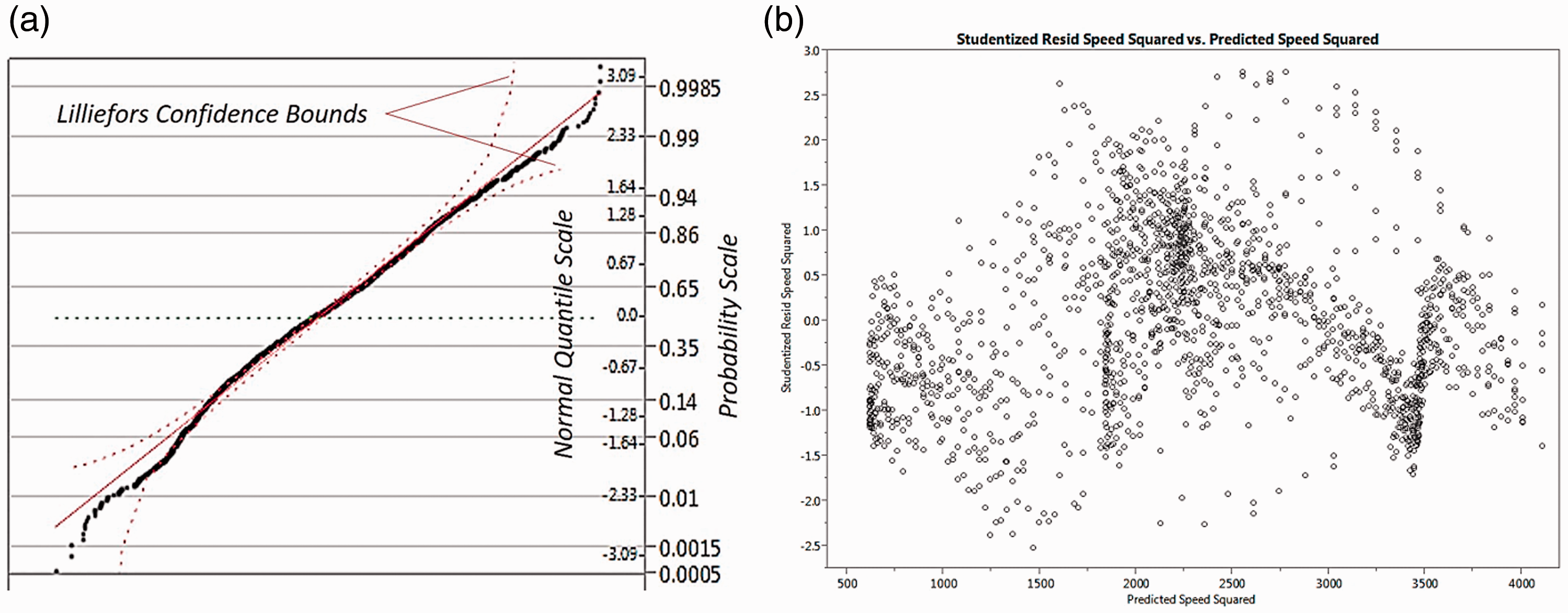
Regression assumption check after data transformation. (a) Normality check: standardized residuals; (b) Heteroscadasticity check.

Heteroscedasticity is generally detected by looking at the scatter plot of the standardized residuals versus the predicted values of the dependent variable. As shown in Figure 4(b), the residuals are randomly spread out without any systematic patterns, which suggest that there is no significant evidence of heteroscedasticity in the proposed model.

Modeling time–speed curves by land use clusters

To produce a reliable prediction model by satisfying all regression assumptions, the outliers over ± 2.7 were detected and excluded from the initial examination. Spearman’s rho test was conducted to examine whether the transformed speed variable is affected by temporal periodicity. The test results confirmed that a predictor contributes to predicting the operational speed data (ρ = ‒.477, p < .0001).

The proposed model is drawn as a centered polynomial model that fits the same curve by reducing a chance to have a high correlation between a predictor (X) and its higher order terms. The concept of centering is to subtract the mean value of X from all X values, i.e. the centered X value is the distance of any X value from the mean of all X values (SAS Institute, 2016). For the proposed model development, the centering value of 13.31 was achieved as the average time slot of the samples.

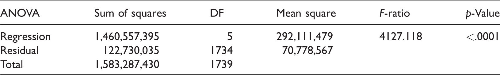
Table 3 shows a summary result of a one-way ANOVA analysis, while Table 4 shows a summary of the regression analysis. The F-ratio of 4157.118 is significant at the .0001 level, which suggests the proposed regression model is adequate. An adjusted R-squared value of .922 indicates a very strong reasonable fit between the operational speed and its prediction attributes, which suggests that 92.2% of variability in the operational speed could be explained by the selected independent variables.

Table 3.

Summary of ANOVA.

ANOVA	Sum of squares	DF	Mean square	F-ratio	p-Value
Regression	1,460,557,395	5	292,111,479	4127.118	<.0001
Residual	122,730,035	1734	70,778,567
Total	1,583,287,430	1739

Table 4.

Summary of quartic polynomial regression analysis.

Parameters	Coefficient	Std. error	t-Value	p-Value	R²	Adj. R²
Constant	6336.92	51.28	123.57	<.0001	0.923	0.922
Time	–302.13	3.76	–80.34	<.0001
(Time – 13.31)²	–37.49	1.39	–26.96	<.0001
(Time – 13.31)³	5.98	0.11	55.60	<.0001
(Time – 13.31)⁴	1.16	0.03	39.03	<.0001
Commercial	–607.44	6.38	–95.22	<.0001
Industrial	607.44	6.38	95.22	<.0001

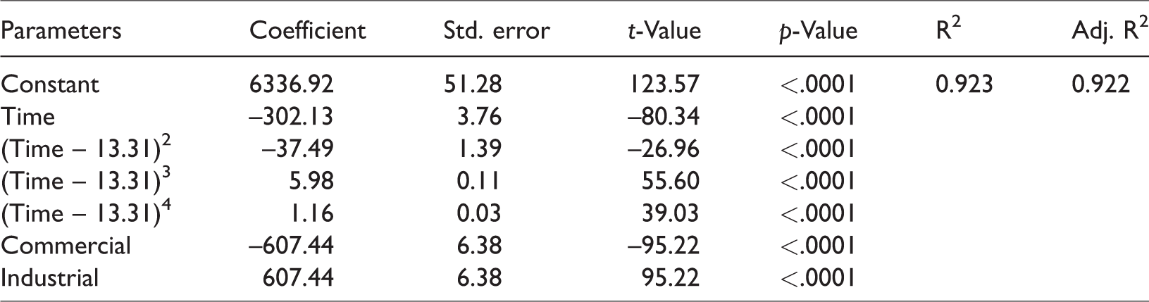
With seven coefficients that are significant, the following centered polynomial regression equation to predict the representative traffic patterns was generated as shown in equation (2) and Figure 5

{Speed}^{2} = 6336.92 - 302.13 \cdot (Time) - 37.49 \cdot {(Time - 13.31)}^{2}

+ 5.98 \cdot {(Time - 13.31)}^{3} + 1.16 \cdot {(Time - 13.31)}^{4} - 607.44 \cdot I_{1}

(2)

where

If I₁ = 1: Commercial land use

If I₁ = ‒1: Industrial land use

Figure 5.

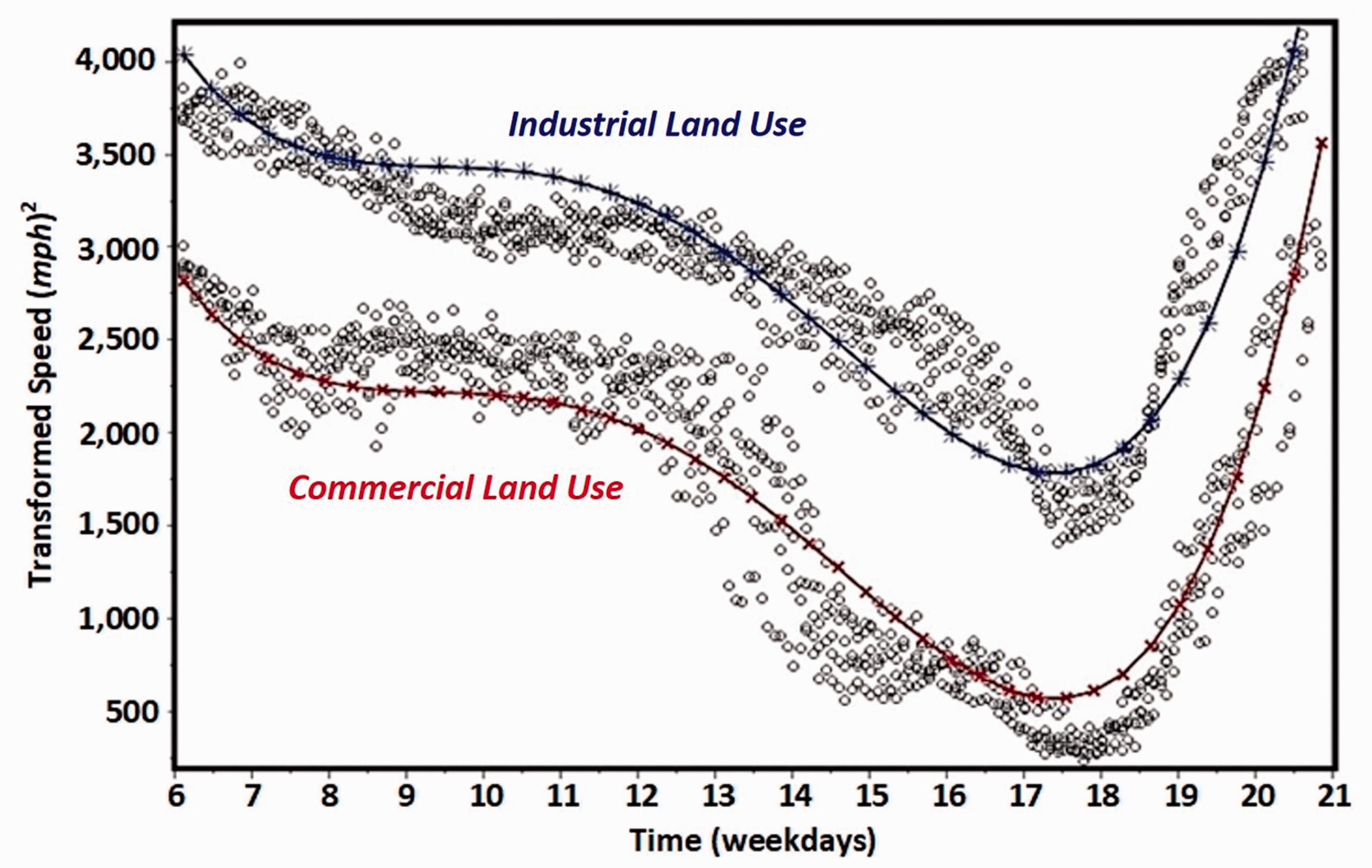
Fitted lines of the developed model.

Two different curved lines for the land use clusters indicate the fitted lines produced by equation (2), while several dots show the corresponding actual travel speed data points used in this modeling process.

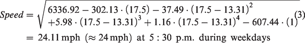
According to the results of the centered quartic polynomial regression model shown in Figure 5, severe traffic congestion was investigated in the commercial use cluster of Downtown LA, compared to the industrial use area along I-10 E. As an example, the p.m. peak hour (5: 30 p.m.) was set to 17.5. Using the set value of time, the expected speed can be calculated as follows (equations (3) and (4))

For the commercial land use cluster (I₁ = 1)

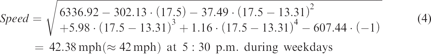
Speed = \sqrt{\begin{array}{l} 6336.92 - 302.13 \cdot (17.5) - 37.49 \cdot {(17.5 - 13.31)}^{2} \\ + 5.98 \cdot {(17.5 - 13.31)}^{3} + 1.16 \cdot {(17.5 - 13.31)}^{4} - 607.44 \cdot (1) \end{array}} = 24.11 mph (≈24 mph) at 5:30 p.m. during weekdays

(3)

For the industrial land use cluster (I₁ = ‒1)

Speed = \sqrt{\begin{array}{l} 6336.92 - 302.13 \cdot (17.5) - 37.49 \cdot {(17.5 - 13.31)}^{2} \\ + 5.98 \cdot {(17.5 - 13.31)}^{3} + 1.16 \cdot {(17.5 - 13.31)}^{4} - 607.44 \cdot (- 1) \end{array}} = 42.38 mph (≈42 mph) at 5:30 p.m. during weekdays

(4)

Validation of the robustness of model

An appropriate approach to validating the robustness of model is critical, especially when developing a statistical model. A typical validation method tests the model with new data sets that are not employed in the modeling process, but it is often limited by the ability to acquire an independent data set (Choi et al., 2012, 2015a, 2015b). This difficulty has been overcome by an alternative validation method that does not need additional new sets of data, i.e. the PRESS statistic (Choi et al., 2012, 2015a, 2015b; Holiday et al., 1995; Ott and Longnecker, 2010; Tarpey, 2000). The PRESS statistic was adopted in this study to test the predictability and accuracy of the model developed here.

PRESS measures the prediction quality based on the comparison between each observed response and the corresponding value based on the fitted model, as shown in equation (5) (Choi et al., 2012, 2015a, 2015b)

PRESS = \sum_{i = 1}^{n} {(y_{i} - {\hat{y}}_{i}^{*})}^{2}

(5)

where

y_{i}

is a prediction for the ith observation in the regression model, and

{\hat{y}}_{i}^{*}

is a prediction of a new subset model for the ith observation, which is fitted with leaving out the ith observation.

The PRESS statistic is then compared with the sum of squared error (SSE), measuring the level of discrepancy between the sum of the squared differences in predicted and actual values (Choi et al., 2012, 2015a, 2015b; Ott and Longnecker, 2010). If the value of the PRESS statistic is closer to the SSE value, it statistically verifies that the proposed model can predict new data with high certainty. The PRESS statistic cannot be smaller than the value of SSE (Ott and Longnecker, 2010). On the other hand, if the PRESS statistic is much larger than the SSE value, it indicates a validation issue in the proposed regression model (Ott and Longnecker, 2010). The ratio of PRESS to SSE values for the proposed traffic speed-time model was 1.002 (PRESS/SSE = 266.5527/266.0424), which indicates that the proposed model is robust in predicting vehicle speeds during the given time period (6:00 a.m. to 9:00 p.m.) during weekdays adjacent to Downtown LA, which consists of commercial and industrial land uses.

Illustrative example: Practical applicability

Caltrans endeavors to sustain service levels at the transition between LOS C and LOS D. Caltrans emphasizes that anything below LOS D can be regarded as unacceptable conditions (Caltrans, 2002). Among LOS for roadways, Table 5 presents LOS for freeway sections based on the criteria of average travel speed (Transportation Research Board, 2010).

Table 5.

Level of service for freeway sections.

LOS	Average travel speed (mph)	Technical description
A	≥60	No delays
B	≥55	No delays
C	≥49	Minimal delays
D	≥41	Minimal delays
E	≥30	Significant delays
F	<30	Considerable delays

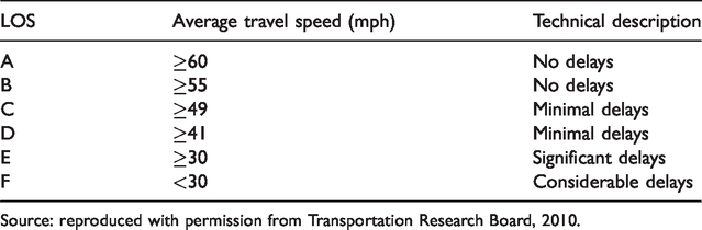
Source: reproduced with permission from Transportation Research Board, 2010.

Based on the LOS rating system, an illustrative example demonstrates how the developed model can be used to capture the LOS during critical time periods by the land use clusters. More specifically, the developed model was applied to capture the time points of minimal delays and significant delays by the land use clusters. As shown in Figure 6, the operational status close to the industrial use area was an acceptable condition during weekdays. However, near the commercial use area, there would be critical periods during weekdays that significantly affect the service.

Figure 6.

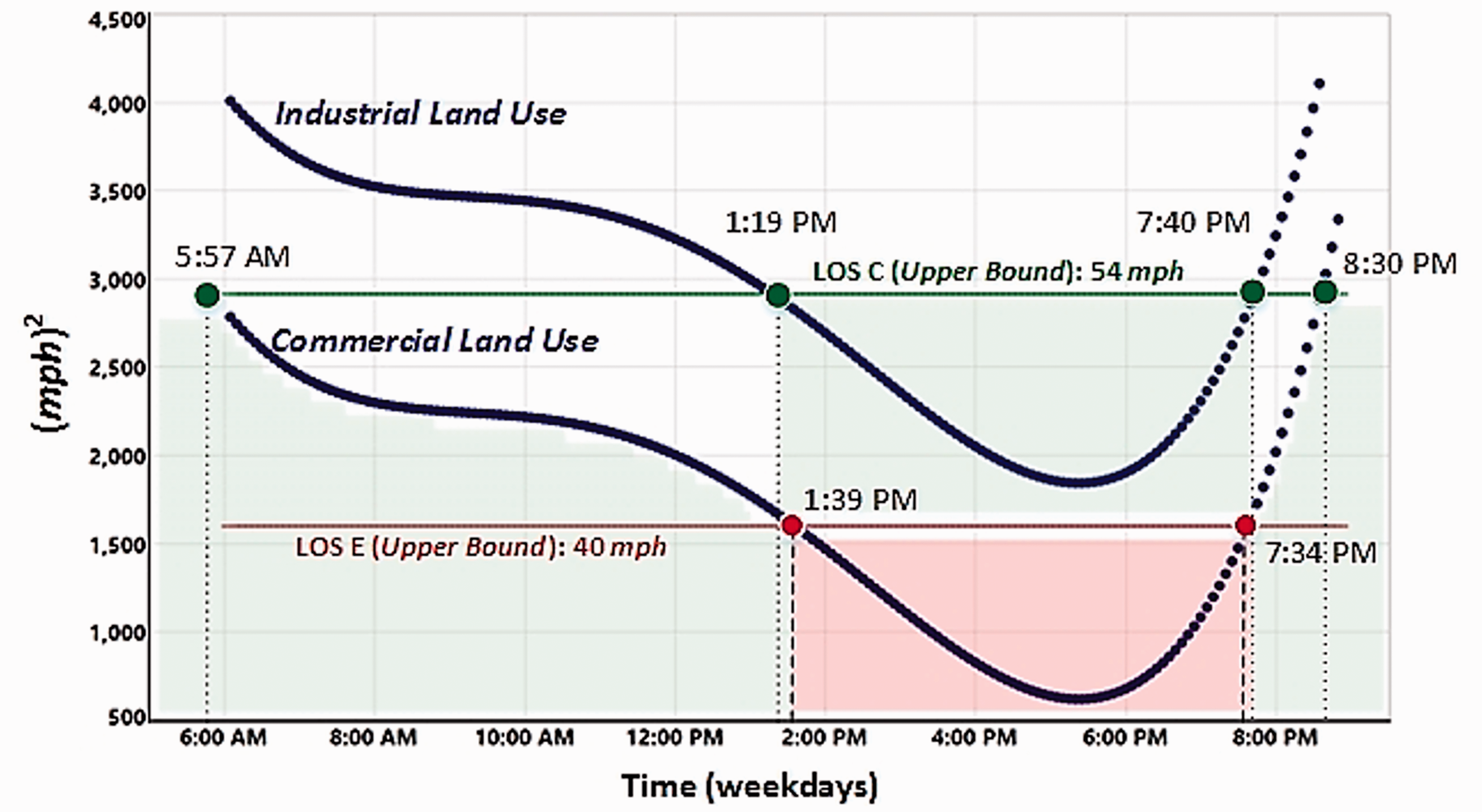
Graphical illustration of LOS by the land use clusters.

Using the proposed regression model, the critical time period in the commercial land use type was detected. As the result, two time points of 13.65 and 19.57 were obtained from the mathematical equation (equation (6))

{(40)}^{2} = 6336.92 - 302.13 \cdot (Time) - 37.49 \cdot {(Time - 13.31)}^{2} + 5.98 \cdot {(Time - 13.31)}^{3} + 1.16 \cdot {(Time - 13.31)}^{4} - 607.44 \cdot 1

(6)

These two values indicate that there would be severe traffic congestion between 1:39 p.m. and 7:34 p.m. during weekdays in the commercial land use cluster along I-10 E, by showing below LOS E.

Conclusions

LOS has been widely used to measure the operational efficiency of existing highway systems categorically, based on certain ranges of traffic speeds. However, this existing method is too broad to investigate urban traffic characteristics. A more effective and efficient method that captures the unique characteristics of LOS during a certain temporal duration in a common spatial area that includes different land uses is needed.

To fill this gap, this study attempted to model the link between traffic speeds and land uses during certain time periods, along with the given LOS criteria. To this end, this study developed and validated a traffic time–speed curve model that includes different land uses in a large urban core. As a case study, this study adopted a CBD in LA in the United States. A total of 1780 sensor readings on I-10 E adjacent to Downtown LA was collected during weekdays (6:00 a.m. to 9:00 p.m.) of the first quarter of a calendar year. The collected data were summarized using a signature-based approach in order to generate traffic flows. Along with the I-10 E roadway network, spatial information was clustered by its land use (i.e. commercial and industrial), which are designated by the zoning regulations of the city of LA. Significant differences in speed in each land use type was investigated and scientifically tested. The result showed that traffic congestion in the commercial land use cluster was higher than in the industrial.

Based on the result, a fourth-order polynomial regression with a categorical variable was conducted to generate a stochastic decision-support model that captures the unique characteristic of spatiotemporal traffic patterns. To detect time intervals that are available to predict the operational status of the I-10 E roadway network adjacent to Downtown LA during the weekdays of the first quarter of a calendar year, the upper bound of LOS E (40 mph of average travel speed) was applied. The finding showed that there would be severe traffic congestion between 1: 39 p.m. and 7: 34 p.m. in the commercial land use cluster along I-10 E adjacent to Downtown LA, by showing below LOS E. In contrast, minimal delays (LOS C) between 1:19 p.m. and 7:40 p.m. were shown in the industrial land use type in Downtown LA. The robustness of the proposed quantitative model was validated by comparing the PRESS statistic with SSE values.

Although this study was temporally limited to the first quarter of a calendar year during particular time intervals and spatially constrained by the CBD, other spatiotemporal traffic patterns could be discovered by following the research method proposed in this study. Specifically, the proposed research method would allow government transportation agencies to predict the most representative traffic patterns that are applicable to any given roadway network associated with particular land use clusters (e.g. residential, business, areas of attraction, and remote areas) within a common spatial area. In summary, this study focused on making recommendations for government transportation agencies to employ an appropriate method that can estimate critical time periods affecting the existing operational status of a highway segment in different land use clusters within a common spatial area. In addition, the main findings of this study also help government transportation agencies promote an effective application of a set of historical traffic sensor speed data, as a way for urban planners to establish an effective strategy or policy that can reduce traffic congestion, compared to other simulation-based methods.

Footnotes

Declaration of conflicting interests

The author(s) declared no potential conflicts of interest with respect to the research, authorship, and/or publication of this article.

Funding

The author(s) received no financial support for the research, authorship, and/or publication of this article.

ORCID iD

Junseo Bae

Junseo Bae is a Lecturer in the School of Computing, Engineering and Physical Sciences at the University of the West of Scotland, UK. He received his PhD from Texas A&M University. His research is centered on developing big-data-driven decision-support modeling frameworks for streamlined transportation infrastructure planning, operation, and management, including (1) road infrastructure informatics, (2) urban infrastructure sustainability, and (3) improved project planning, delivery, and management strategies.

Kunhee Choi is an Associate Professor and holder of the Cecil Windsor Endowed Professorship in Construction Science at Texas A&M University, USA. He earned his PhD from the University of California at Berkeley. His research interests include (1) decision-support civil informatics for autonomously predicting mobility and safety impacts of urban highway rehabilitation works, (2) performance analysis of different types, sizes, and complexities of highway projects, and (3) construction economics, financing, and valuations.

References

Alameda County Transportation Commission (2012) Level of service report. Available at: www.alamedactc.org/app_pages/view/8091 (accessed 18 July 2020).

Anderson

Kanaroglou

Miller

, et al. (1996) Simulating automobile emissions in an integrated urban model. Transportation Research Record: Journal of the Transportation Research Board 1520: 71–80.

Bae

Choi

(2017) Multicontextual machine-learning approach to modeling traffic impact of urban highway work zones. Transportation Research Record: Journal of the Transportation Research Board 2645; 1: 184–194.

Ben-Akiva

Bierlaire

Koutsopoulos

, et al. (1998) DynaMIT: A simulation-based system for traffic prediction. In: DACCORS short term forecasting workshop, Delft, The Netherlands. Citeseer.

Bhuyan

Nayak

(2013) A review on level of service analysis of urban streets. Transport Reviews 33: 219–238.

Caltrans (2002) Guide for the Preparation of Traffic Impact Studies. Sacramento, CA: Caltrans.

Caltrans (2019) The Caltrans Performance Measurement System (PeMS). Available at: http://pems.dot.ca.gov/ (accessed 18 August 2020).

Chaudhuri

Clarke

(2015) On the spatiotemporal dynamics of the coupling between land use and road networks: Does political history matter? Environment and Planning B: Planning and Design 42: 133–156.

Chen

Petty

Skabardonis

, et al. (2001) Freeway performance measurement system: Mining loop detector data. Transportation Research Record: Journal of the Transportation Research Board 1748(1): 96–102.

10.

Choi

Haque

Lee

, et al. (2012) Macroeconomic labour productivity and its impact on firm’s profitability. Journal of the Operational Research Society 64(8): 1258–1268.

11.

Choi

Kim

Bae

, et al. (2015a) Determining future maintenance costs of low-volume highway rehabilitation projects for incorporation into life-cycle cost analysis. Journal of Computing in Civil Engineering 30: 04015055.

12.

Choi

Lee

Bae

, et al. (2015b) Time-cost performance effect of change orders from accelerated contract provisions. Journal of Construction Engineering and Management 142: 04015085.

13.

Cornell University (2008) Statistical Consulting News Archives. Available at: www.cscu.cornell.edu/news/statnews/stnews72.pdf (accessed 18 August 2020).

14.

Das

Pandit

(2016) Methodology to determine service delivery levels for public transportation. Transportation Planning and Technology 39: 195–217.

15.

Department of City Planning-City of Los Angeles (2006) Genralized summary of zoning regulations. Available at: http://planning.lacity.org/ (accessed 18 August 2020).

16.

Dowling

Flannery

Landis

, et al. (2008) Multimodal level of service for urban streets. Transportation Research Record: Journal of the Transportation Research Board 2071(1): 1–7.

17.

Ermagun

Levinson

(2019) Development and application of the network weight matrix to predict traffic flow for congested and uncongested conditions. Environment and Planning B: Urban Analytics and City Science 46: 1684–1705.

18.

Ghods

Saccomanno

(2016) Evaluation of level-of-service measures for two-lane highways with a simulation model. Transportation Research Record: Journal of the Transportation Research Board 2553(1): 20–28.

19.

Handy

(2005) Smart growth and the transportation-land use connection: What does the research tell us? International Regional Science Review 28: 146–167.

20.

Harding

Patterson

Miranda-Moreno

, et al. (2014) A spatial and temporal comparative analysis of the effects of land-use clusters on activity spaces in three Quebec cities. Environment and Planning B: Planning and Design 41: 1044–1062.

21.

Hasley

(2013) Washington rated the worst for traffic congestion. Available at: www.washingtonpost.com/local/trafficandcommuting/washington-rated-the-worst-for-traffic-congestion–again/2013/02/04/125be724-6ee3-11e2-8b8d-e0b59a1b8e2a_story.html (accessed 18 August 2020).

22.

Holiday

Ballard

McKeown

(1995) PRESS-related statistics: Regression tools for cross-validation and case diagnostics. Medicine and Science in Sports and Exercise 27: 612–620.

23.

Hourdakis

Michalopoulos

Kottommannil

(2003) Practical procedure for calibrating microscopic traffic simulation models. Transportation Research Record: Journal of the Transportation Research Board 1852: 130–139.

24.

Hunt

Simmonds

(1993) Theory and application of an integrated land-use and transport modelling framework. Environment and Planning B: Planning and Design 20: 221–244.

25.

Jafarzadeh

Wilkinson

González

, et al. (2013) Predicting seismic retrofit construction cost for buildings with framed structures using Multi-Linear regression analysis. Journal of Construction Engineering and Management 140(3).

26.

Jolovic

Stevanovic

(2012) Evaluation of vissim and freeval to assess an oversaturated freeway weaving segment. In: TRB 91st annual meeting. Transportation Research Board, January 22 - 26, Washington, D.C. p.12.

27.

Jolovic

Stevanovic

Sajjadi

, et al. (2016) Assessment of level-of-service for freeway segments using HCM and microsimulation methods. Transportation Research Procedia 15: 403–416.

28.

Kamarianakis

Prastacos

(2005) Space–time modeling of traffic flow. Computers & Geosciences 31: 119–133.

29.

Kanaroglou

(1999) New transportation links and urban air quality: In: 6th international conference on environmental science and technology, Pythagorion, Samos, Greece. Hamilton, ON: The Red Hill Creek Expressway.

30.

Karim

Adeli

(2003) CBR model for freeway work zone traffic management. Journal of Transportation Engineering 129: 134–145.

31.

Lowry

Balling

(2009) An approach to land-use and transportation planning that facilitates city and region cooperation. Environment and Planning B: Planning and Design 36: 487–504.

32.

Duan

Kang

, et al. (2015) Traffic flow prediction with big data: A deep learning approach. IEEE Transactions on Intelligent Transportation Systems 16: 865–873.

33.

Maat

Van Wee

Stead

(2005) Land use and travel behaviour: Expected effects from the perspective of utility theory and activity-based theories. Environment and Planning B: Planning and Design 32: 33–46.

34.

Nilsson

Smirnov

(2016) Measuring the effect of transportation infrastructure on retail firm co-location patterns. Journal of Transport Geography 51: 110–118.

35.

Ott

Longnecker

(2010) An Introduction to Statistical Methods and Data Analysis. Pacific Grove, CA: Brooks/Cole.

36.

Pendyala

Konduri

Chiu

Y-C

, et al. (2012) Integrated land use–transport model system with dynamic time-dependent activity–travel microsimulation. Transportation Research Record: Journal of the Transportation Research Board 2303: 19–27.

37.

Ramadan

Sisiopiku

(2016) Impact of bottleneck merge control strategies on freeway level of service. Transportation Research Procedia 15: 583–593.

38.

Rao

(2012) Measuring urban traffic congestion – A review. International Journal for Traffic & Transport Engineering 2(4): 286–305.

39.

Romero

(2015) 6 of the 7 worst stretches of freeway are in L.A., but Chicago makes the 405 look speedy. Available at: www.laweekly.com/news/6-of-the-7-worst-stretches-of-freeway-are-in-la-but-chicago-makes-the-405-look-speedy-6308826 (accessed 18 August 2020).

40.

SAS Institute (2016) Usage note 37925: Why does JMP® center polynomials in models by default? Available at: www.jmp.com/support/notes/37/925.html (accessed 18 August 2020).

41.

Spiegelman

Park

Rilett

(2011) Transportation statistics and microsimulation. Boca Raton, FL: Champman & Hall/CRC.

42.

State of California (2001) A citizen’s guide to planning. Available at: www.acgov.org/sustain/documents/CitizensGuidetoLandUsePlanninginCalifornia.pdf (accessed 18 August 2020).

43.

Strauch

Moeckel

Wegener

, et al. (2005) Linking transport and land use planning: The microscopic dynamic simulation model ILUMASS. In: Peter Atkinson, Giles M. Foody, Steven E. Darby, Fulong Wu (eds), Geodynamics, FL: CRC Press.,pp.295–311.

44.

Strong

Lee

Wang

(1997) Data quality in context. Communications of the ACM 40: 103–110.

45.

Tarpey

(2000) A note on the prediction sum of squares statistic for restricted least squares. The American Statistician 54: 116–118.

46.

Taubenböck

Klotz

Wurm

, et al. (2013) Delineation of central business districts in mega city regions using remotely sensed data. Remote Sensing of Environment 136: 386–401.

47.

Transportation Research Board (2010) Highway Capacity Manual (HCM2010). Washington, DC: Transportation Research Board.

48.

TRIP (2014) California transportation by the numbers: Meeting the State’s need for safe and efficient mobility. Available at: www.tripnet.org/docs/CA_Transportation_by_the_Numbers_TRIP_Report_Sep_2014.pdf (accessed 18 August 2020).

49.

Van Lint

Hoogendoorn

Van Zuylen

(2002) Freeway travel time prediction with state-space neural networks: Modeling state-space dynamics with recurrent neural networks. Transportation Research Record: Journal of the Transportation Research Board 1811: 30–39.

50.

Waddell

(2002) UrbanSim: Modeling urban development for land use, transportation, and environmental planning. Journal of the American Planning Association 68: 297–314.

51.

Wang

Reddy

Kon

(1995) Toward quality data: An attribute-based approach. Decision Support Systems 13: 349–372.

52.

Zhu

Ahmad

Wang

(2009) Estimating work zone road user cost for alternative contracting methods in highway construction projects. Journal of Construction Engineering and Management 135: 601–608.

A land-use clustering approach to capturing the level-of-service of large urban corridors: A case study in downtown Los Angeles

Abstract

Keywords

Introduction

Level-of-service: A congestion measurement method

Point of departure: Knowledge gaps

Employing quality data

Linking land use clusters to critical time–speed estimation

Research objectives and methods

Data collection and classification

Initial data analysis: Average travel speed versus land use

Modeling the link between highway traffic speed and land use

Designing a quartic polynomial regression model

Modeling time–speed curves by land use clusters

Validation of the robustness of model

Illustrative example: Practical applicability

Conclusions

Footnotes

Declaration of conflicting interests

Funding

ORCID iD

References