Sage Journals: Discover world-class research

Abstract

Traffic congestion is a major environmental and social problem whose causes include urban sprawl, imbalanced home-job distributions, increased car ownership, and lack of public transportation. We focus on a relatively understudied factor: the existence of geographic barriers. We study traffic times and flows in the Boston metropolitan area, a major coastal city with substantial shape non-convexities. We show that natural barriers not only cause additional delays to the trips affected directly, but also worsen downtown congestion for everyone. Additionally, commuter flows between places separated by barriers decrease, generating additional traffic elsewhere. We also find that places next to geographic obstacles suffer from higher risks of congestion, due to their lower traffic-diffusion ability. Policymakers may consider specific solutions for congestion arising from constraining physical geographies.

Keywords

Traffic congestion physical barriers commuting patterns

Introduction

The economic and personal development of the urban dweller relies critically on their access to jobs (Ganin et al., 2017; Horner 2004; Massaro et al., 2018; White 1986; Zhang et al., 2019). However, commuting costs keep growing (Zhou et al. 2020). Increasing car use and traffic congestion have detrimental impacts on environmental degradation (Chapman 2007; Figliozzi 2011; McGovern 1998; Morawska et al., 2008) and energy consumption (De Vlieger et al., 2000). They also worsen inequality (Stokes and Seto 2018), mental health (Hansson et al., 2011), and reduce time spent with family (Green et al., 1999). Because congestion shows no signs of abating, its avoidance generates durable impacts on human behavior. These include residential choices, driving speed, departure times, and routing (Arnott et al., 1992; Wang et al., 2016).

In parallel, the scientific measurement of travel and locational behavior has improved (Huang et al., 2018). Large excess commuting (EC)—computed by comparing peak-time trip duration to a theoretical minimum (Hamilton and Röell, 1982)—is now routinely detected in multiple environments (Black et al., 2002; Horner, 2004; Zegras, 2010). Extant studies have explored the determinants of EC and identified a few critical ones, mostly having to do with individual car usage and urban sprawl (see Appendix, Brief Annotations on Literature on Determinants of Excess Commuting).

However, as pointed by Giuliano and Small (1993), there are other factors beyond behavioral and land-use ones that remain relatively unexplored. For example, the useful conceptual assumption that city roads are radially distributed from the city center into suburban areas—which is the theoretical base of most of the literature in urban economics (Hamilton and Röell, 1982; Hamilton, 1989; Wheaton, 2004)—is empirically lacking. Arguably, research in transportation and environmental planning has also understudied the impact of traffic constrains caused by complex geographic features. An important strand of the literature has investigated the relationship between urban shape and urban outcomes, but mostly focusing on aspects that have to do with human agency in land use—density, compactness, or sprawl, as in (Carruthers and Ulfarsson, 2003; Rolheiser and Dai, 2019; Miranda, 2020). Research has also delved into the measurement of city shapes and their growth (Angel et al., 2010; Amindarbari and Sevtsuk; 2012; Batty, 2008). Naturally, current city shapes result from a combination of geographic, historical, economic, and planning factors.

Other research looks more specifically into the impact of a difficult physical geography on urban outcomes. Saiz (2010) demonstrates that a constraining geography—due to steep terrain, oceans, and internal bodies of water—affects the supply of urban housing. Constrained cities need to expand further in order to accommodate the same amount of people at similar densities. Alternatively, profitable development at higher densities closer to the city center requires of more expensive land (Ahlfeldt and McMillen, 2018). Harari (2020) finds that cities with compact geographies are associated with faster population growth, higher productivity, and better quality of life in India. These findings have been replicated in Latin America by Duque et al. (2019). Angel and Franco (2018) theorizes about the impacts of urban shapes, and concludes that both population density and compactness should affect travel distances. This hypothesis is confirmed by Akbar et al. (2018), who compare average commuting outcomes across cities in India. These authors find that the shape non-convexities induced by hilly terrain and water bodies are associated with slower traffic on average. In addition, geographical barriers also beget more congestion during peak commuting times. Akbar et al (2021). replicate these results in a global sample of 1200 cities.

While the comparative literature is conclusive about the “macro” challenges experienced by cities with irregular geographies, there has been scarce work on the mechanisms mediating these effects within urban areas. In this paper, we focus on the Boston metropolitan area—a globally important coastal region with major shape non-convexities—as a case study. We gather, analyze, and compare data from thousands of individual trips, substantively covering the whole metropolitan area. We hence can shed light on how geographically induced non-convexities affect trip characteristics at “micro” and “meso” levels (Zegras, 2010).

We hypothesize and empirically confirm four distinct effects of physical-geography barriers on commuting outcomes, which go beyond those in (Saiz, 2010). (1) Naturally, barriers between two points in the city increase the length and duration of the driving trip between them. Using the terminology in (Cole and King, 1968), detour factors—the ratio between minimum road trip distance and euclidean (straight-line) distance—must increase in order to circumvent natural barriers. While conceptually straightforward, the extent of this effect is not usually quantified. In the paper, we provide a parsimonious way for doing so. (2) Less obviously, urban shape non-convexities induced by natural barriers can derive additional trips into the city center, thereby increasing traffic externalities precisely where it is most congested and more people are affected. (3) The existence of natural barriers between two points reduces their dyadic commuting flows, counterfactually displacing traffic to other locales. This effect generates a more uneven distribution of commutes within the city. (4) The low traffic-diffusion ability of the roads that are close to the coast or other natural barriers renders them more susceptible to congestion at peak times or when accidents happen.

The paper proceeds as follows. In section 2, we describe the data on trip qualities and commuting flows. We also provide details about the empirical specifications that we deploy in the paper. Section 2 measures the extent of the basic detour effect (#1), and also provides evidence of significant rerouting through the city center (effect #2). In this section, we also demonstrate that trips that should run in directions that are interrupted by natural features are longer and slower. Section 3 focuses on effect #3. We use data on point-of-employment and place-of-residence from the Census and show clear evidence of reduced commuting between points that are mutually harder to access. Section 4 develops a conceptual framework inspired by basic thermodynamics to study congestion in areas adjacent to barriers. We then test and validate the implications of that framework, finding that traffic flowing in proximity to oceans is more prone to congestion peaks. Section 5 concludes.

Data and methods

Data

In order to explore empirically the aforementioned effects, we use the OpenStreetMap’s application programming interface (API) to calculate the mileage of the shortest distance path (SDP) between a number of representative points throughout the city (Appendix. Urban roads). These 147 reference points are separated by 1 km along eight directional axes from Boston’s downtown, at intervals of 45° from true-bearing (Appendix. Spatial partition strategy). The strategy is computationally feasible, allows us to capture representative traffic patterns from alternative geographic directions—covering most of the proximate metropolitan area—and avoids the duplication of overlapping trips (Figure 1). SDPs between all 21,462 combinations of our reference commuting origins and destinations capture the absolute minimum driving distance between any two points. The shortest path is not always the one used by drivers, due to congestion, street design, or traffic impediments (Tang and Levinson, 2018; Zhu and Levinson, 2015). Nonetheless, this variable provides a lower bound for the trip’s mileage.

Figure 1.

Location and geographic features of Boston. The outer red circle defines the radius of the study area, 25 km. The inner red circle captures points at 5 km or less from the city’s commercial center. Maps of the distribution of the 147 study points (defined in Appendix. Spatial partition strategy and Appendix Figure A1) and barriers in the whole Boston are displayed. The frequency distributions of the geographic barriers are shown in the Appendix. Table A3. The commuting patterns between all study-point dyads are analyzed, effectively covering the whole metro area with—by design—better coverage of trips closer to the city center.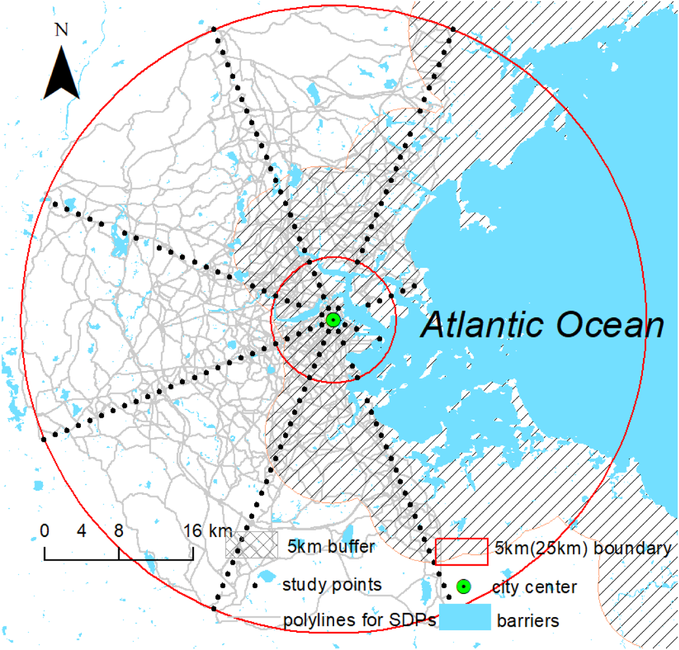

Following Akbar and Duranton (2017) and Akbar et al. (2018) we use Google Maps’ API to find peak driving times between points (at 8 a.m.), or their daily averages (Appendix. Vehicle traveling data). Google provides us with the route that minimizes driving times between locations. Given the very high quality of their algorithm (He et al., 2019), we interpret this variable as capturing the shortest time path (STP) driving duration.

We use GIS data from the United States Geographic Service (USGS) about oceans, internal bodies of water, and steep terrain (Appendix. Geographic barriers)—at slopes above 15°, as in (Saiz 2010). We then calculate the euclidean straight-line distance (SLD) between all origin-destination pairs. Combining the two measurements, we calculate the share of the straight-line segment between points that is transected by the ocean or by terrain with slopes above 15% (the latter being a rare occurrence in the Boston area). This metric—measured at the trip level—is a local empirical counterpart to the mathematical concept of convexity. A convex set is such that the linear segment uniting two points is fully contained within the set. In our definition, larger shares of that segment intersected by barriers imply more local non-convexity.

As can be seen in Figure 1, the main geographical barriers are for trips between points to the east of the city center and in proximity to the coast. The ocean generates substantial non-convexities in the city’s land shape While our numerical estimates are specific to Boston, they exemplify a broader phenomenon applicable to other coastal cities. Many of them expanded around a well-located natural harbor: a bay or other water inlet. Because the water bulges into the land, many points are effectively separated by a geographical barrier that has to be circumvented by the way of longer commutes.

An additional two geographic data measurements required downloading all SDP 10,731 polylines from OpenStreetMap. We subsequently used GIS software (ArcGIS Pro 2.5) to overlay them to 5-km buffers around the coastal line, and around the city’s downtown. This allows us to calculate the share of both the SDP—and also the SLD—that flow through central or coastal areas.

Finally, we also deploy the US census Longitudinal Employer-Household Dynamics (LEHD) Origin-Destination Employment Statistics (LODES) data set (Appendix. Employment data) to measure the intensity of commuter trips between points. Concretely, we assign trips to the catchment areas of origin-destination pairs if they depart and arrive, respectively, in census blocks with centroids within 5 km of both the origin and destination points (Appendix. Spatial smoothing of commuting flows and Appendix. Figure A2). This allows us to have a broad measure of traffic intensity—as opposed to a noisier metric based on a small numbers of commutes between narrowly defined blocks. As in most spatially smoothed measures, the same trip may be assigned to two or more adjacent points that overlap: when this happens, we weight the flows inversely to the degree of the overlap. Because of spatial smoothing, we are careful to use this variable as a relative measure of the local statistical density distribution of commutes—as opposed to an exact absolute count.

Empirical methods

We deploy four distinct types of statistical regression model. Dependent variables always measure a single outcome for each trip between all potential origins and destinations. In the first specification, the main independent variable is the share of the straight-line between origin and destination points that is transected by geographic barriers, denoted below by $S B_{i j}$ . Subscripts $i$ and $j$ throughout are for origin and destination points, respectively. As explained earlier, $S B_{i j}$ is our local measure of topological non-convexity.

y_{i j} = α + β \cdot {S B}_{i j} + Θ X_{i j} + Ω Z_{i} + Ψ Z_{j} + ε_{i j}

(1)

In equation (1), $X_{i j}$ represents a vector of trip characteristics; $Z_{i}$ and $W_{i}$ are—respectively— origin and destination attributes; and $ε_{i j}$ is the error term. We allow for nonzero covariances between trips originating from or arriving to the same points, and thus cluster standard errors two ways correspondingly. The other symbols in (1) capture the independent variables’ parameters. The outcomes of interest here—denoted by $y_{i j}$ —are, respectively, the log of each trip’ SDP mileage and the share of the SDP running through the city center.

We include the following variables as controls: (i) the log of the SLD between points, as we are focusing on capturing effects on traffic outcomes beyond those trivially accounted for by euclidean distances; (ii) the share of the SLD running through the city center, which should affect both the local configuration of the street system and—naturally—the expected share of the SDP transecting central areas; (iii) dummies for whether the trip origin or destination are within 5 km of the ocean;¹ and (iv) respectively, the logs of the overall numbers of commuter trips departing from and arriving to each origin and destination: traffic outcomes between busy locales should differ from those between unpopular destinations.

The second empirical specification in the paper takes the form

y_{i j}^{*} = α^{*} + β^{*} \cdot ({l o g S D P}_{i j} - {l o g S L D}_{i j}) + Θ^{*} X_{i j} + Ω^{*} Z_{i} + Ψ^{*} W_{j} + ε_{i j}^{*}

(2)

The notation here is similar to equation (1), but now the main independent variable is $(\log S D P_{i j} - \log S L D_{i j})$ . This variable corresponds to the percentage increase in SDP milage with respect to the SLD—or approximately one minus the detour factor. It captures how much the milage that a commuter must drive deviates from the distance between origin and destination as-the-crow-flies. Differences between the logs of the SDP and SLD are driven by two factors: (i) idiosyncrasies in the design of the road network; (ii) geographical barriers. Because we are only interested in the variation arising from the latter, we deploy an Instrumental Variables (IV) approach. Concretely, we use the share of the SLD between each origin and destination that is impeded by a natural barrier $S B_{i j}$ as an instrument for our key detour variable.

The outcomes—the dependent variables $y_{i j}^{*}$ in equation (2)—are the logs of Google Maps’ STPs estimated duration and speed. Under the appropriate Local Average Treatment effect (LATE) interpretation (Angrist et al., 1996), the estimates yield the percentage point increase in trip time—or speed—corresponding to a geographically motivated trip detour that amounted to 1% of the SLD.

A second IV specification controls for origin and destination fixed effects (which we denote by $D_{i}$ and $D_{j}$ ). Consequently, we drop the variables measured at those levels:

y_{i j}^{*} = β^{* *} \cdot ({l o g S D P}_{i j} - {l o g S L D}_{i j}) + Θ^{* *} X_{i j} + \sum α_{i} D_{i} + \sum α_{j} D_{j} + ε_{i j}^{* *}

(3)

An additional outcome variable that we study using model (3) is the log of actual commuter trips between points.

Finally, our last specification focuses on the effects of driving through coastal routes:

t_{i j} = {γ S D C}_{i j} + μ \cdot {l o g S D P}_{i j} + λ \cdot {S h L c c}_{i j} + \sum {\hat{a}}_{i} D_{i} + \sum {\hat{a}}_{j} D_{j} + ξ_{i j}

(4)

In equation (4), $S D C_{i j}$ —the main explanatory variable—is the share of the SDP between points that runs within a 5-km buffer of the ocean. The outcomes (captured by $t_{i j}$ ) are the log of estimated driving peak times, or the difference between the logs of peak and daily-average commuting times. We control for the share of the straight line between points traversing the busy city center $(S h L c c_{i j})$ and for the log of the SDP mileage between commuting origins and destinations. Thus, these regressions take as given that the effective trajectories between topologically obstructed points display larger detour factors, and therefore longer SDPs.² Nevertheless, note that many coastal routes will not be obstructed by the ocean, but run in parallel to it. Note further that the fixed effects in (4) imply that all the data variation comes from the researcher-induced quasi-random combinations of routes.

Effect of geographical barriers on commuting outcomes and downtown congestion

Table 1 presents our initial results. Column 1 quantifies the average direct detour effect of barriers in this context. The results suggest that two coastal points separated by a straight-line that lies fully in the ocean can expect a trip that is—at least—30.5% longer than a trip between unobstructed locations.

Table 1.

Impacts of geographic barriers on commuting patterns.

Variables	Log shortest distance path	Share of shortest distance path within 5 km of center	Log duration of Google STP at 8 a.m.	Log trip speed of Google STP at 8 a.m.	Log duration of Google STP at 8 a.m.	Log trip speed of Google STP at 8 a.m.
Variables	(1)	(2)	(3)	(4)	(5)	(6)
Share of straight line distance intersected by geographic barriers	0.305***	0.412***	—	—	—	—
	(0.028)	(0.029)	—	—	—	—
(Log shortest distance path—log straight line distance)^a	—	—	0.716***	-0.497**	1.158***	-0.885***
(Log shortest distance path—log straight line distance)^a	—	—	(0.213)	(0.242)	(0.244)	(0.299)
Log straight line distance	0.878***	0.008***	0.822***	0.153***	0.914***	0.078**
Log straight line distance	(0.006)	(0.003)	(0.027)	(0.031)	(0.033)	(0.039)
Share of straight line route within 5 km of center	-0.074***	0.840***	-0.051	0.015	-0.011	0.0004
Share of straight line route within 5 km of center	(0.012)	(0.014)	(0.038)	(0.043)	(0.030)	(0.0315)
Trip origin is within 5 km of ocean	0.003	0.019***	0.014	-0.025	—	—
Trip origin is within 5 km of ocean	(0.008)	(0.005)	(0.020)	(0.024)	—	—
Trip destination is within 5 km of ocean	-0.025***	0.018***	0.050**	-0.037	—	—
Trip destination is within 5 km of ocean	(0.006)	(0.003)	(0.024)	(0.023)	—	—
Log number of commuter trips originating from origin’s catchment area	-0.049***	0.002	0.118***	-0.102***	—	—
	(0.010)	(0.004)	(0.028)	(0.028)	—	—
Log number of commuter trips arriving in destination’s catchment area	-0.032***	0.011***	0.223***	-0.236***	—	—
	(0.005)	(0.003)	(0.020)	(0.021)	—	—
Constant	1.244***	-0.136***	-5.873***	6.277***	-2.986***	3.319***
Constant	(0.110)	(0.045)	(0.413)	(0.430)	(0.103)	(0.118)
Method (Main independent variable)	OLS	OLS	IV	IV	IV	IV
Adjustment for covariance within	2-way	2-way	2-way	2-way	Fixed	Fixed
Origin/Destinations	cluster s.e	cluster s.e	cluster s.e	cluster s.e	Effects	Effects
R-squared	0.978	0.922	0.843	0.518	0.925	0.731
Kleibergen-Paap wald F STATISTIC	−	−	118.24	118.24	78.13	78.13
Stock-Yogo critical value (10% maximal IV size)	—	—	16.38	16.38	16.38	16.38
Observations (origin-destination combinations)	21,462	—

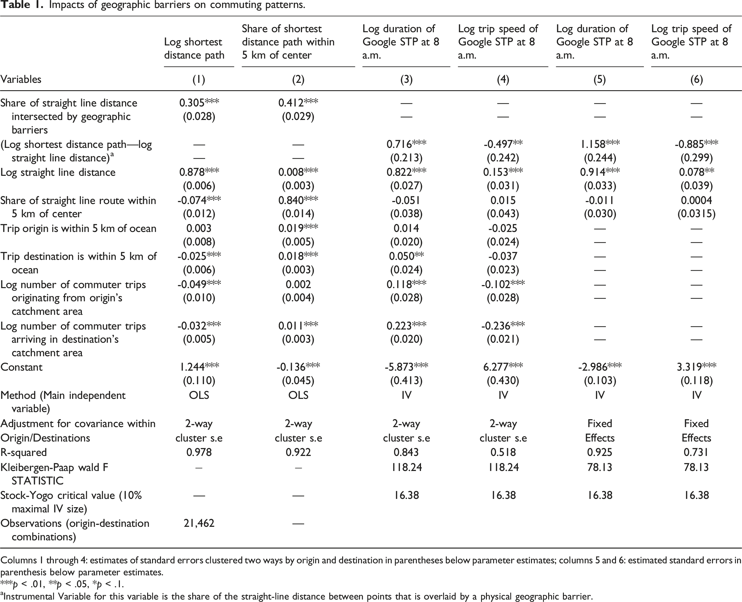
Columns 1 through 4: estimates of standard errors clustered two ways by origin and destination in parentheses below parameter estimates; columns 5 and 6: estimated standard errors in parenthesis below parameter estimates.

***p < .01, **p < .05, *p < .1.

^aInstrumental Variable for this variable is the share of the straight-line distance between points that is overlaid by a physical geographic barrier.

Additionally, coastal cities that expanded out from harbors may suffer additional traffic problems from non-convexities. In many such cities—historically situated on natural bays—the ocean bulges into the land and the city center is located at the inner vertex. Therefore, trips originating and finishing in areas proximate to the ocean have their SDPs routes forced through downtown, increasing congestion there (as in between A and B in Figure 2). We denominate this externality as the effect #2 of natural barriers. Conversely, lateral trips between points that are away from the ocean—in Boston’s case, west of the city—can largely avoid the city center (C and D in the graph).

Figure 2.

Effects #1 and #2 of natural barriers—longer trips and detour into the city center. The purple path shows the SDPs route between A and B, two points in our sample proximate to the ocean. The green path shows the SDPs path between C and D, two sample points away from the ocean. Points are symmetrically distributed from the city center. The SDP path between A and B is closer to the straight line path–denoted by a dash line—and away from the city center. In contrast, the SDP between C and D is substantially longer than the straight line path and is forced through city center.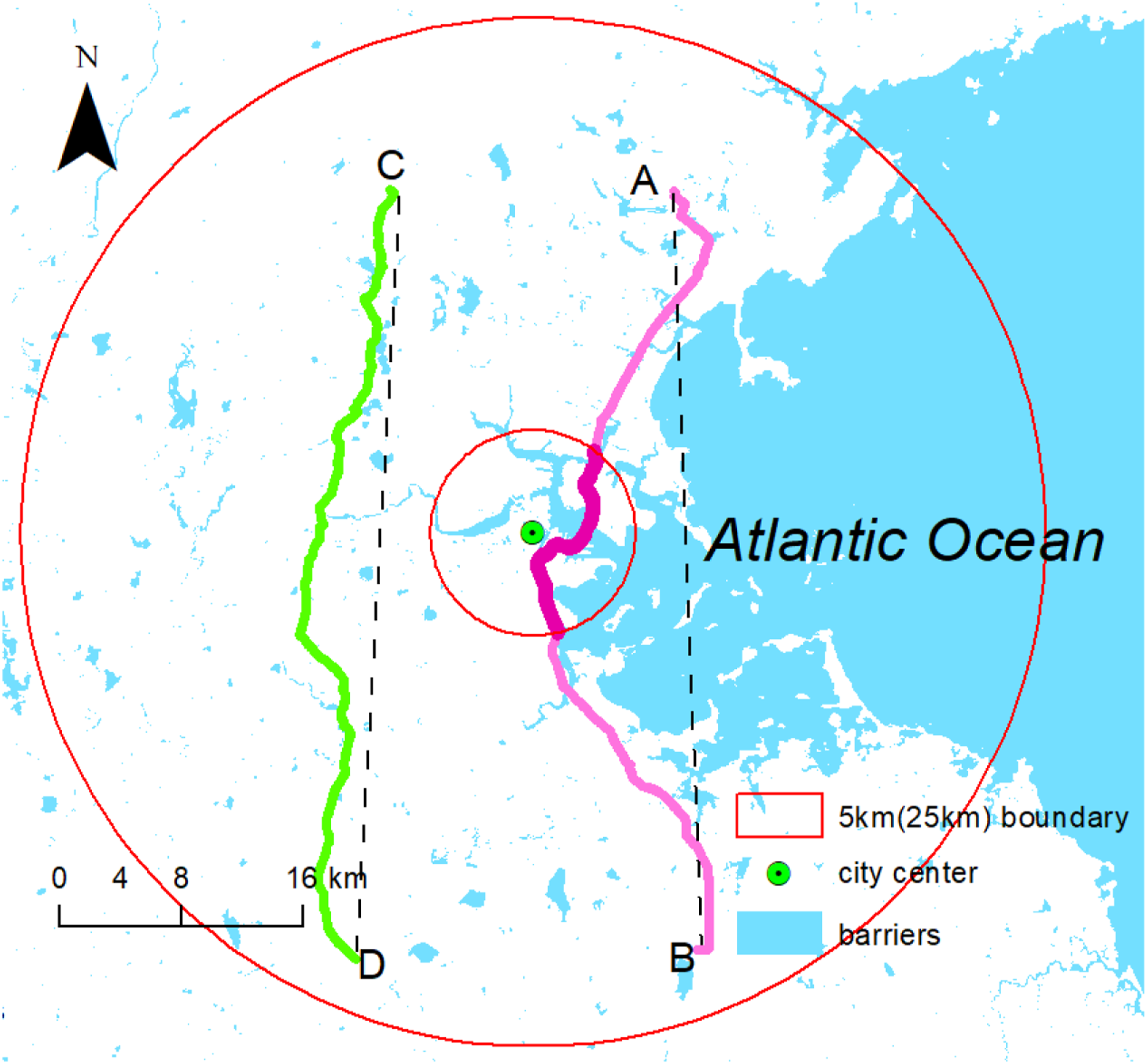

The results in Table 1, column 2 demonstrate the strength of effect #2, with an average elasticity of the share of downtown SDP with respect to the share of barriers of 0.41. This implies that two points with a connecting straight-line that is—for instance—50% impeded by barriers have an average 20.5% -point larger share of their SDP derived into the city center—compared to two unobstructed points. These results show that a difficult physical geography not only delays the trips affected directly; it can also introduce downtown congestion arising from trips that could have taken a more decentralized route absent barriers.

How many more commuter trips are forced into downtown Boston due to its geography? The answer to this question depends on the spatial distribution of commuters’ homes relative to jobs. In order to make a calculation, we use the Census LODES data on commuting trips between each origin (Appendix. Figure A3) and destination (Appendix. Figure A4). From these data, we can infer the SDP downtown kilometers that the average commuter—weighted by trip frequency—is expected to traverse. This figure amounts to 2.89 km. We then estimate how many of these average downtown-routed kilometers are forced by geography. We do so by multiplying each trip’s straight-line barrier share by the average impact of barriers on the downtown share of the SDP—from the first row in Table 1 column 2—and then by each trip’s SDP total. The average of this figure—weighted by the commuting flow frequencies between points—amounts to 0.401 kms, or 13.87% of the total traffic in the center: more than one in 10 trips within the city’s core could have been avoided absent geographical constraints.

The SDP provides us with a lower bound for the extra distance imposed to commuters by geographical barriers. Nonetheless, we are interested in analyzing other conventional commuting metrics—such as driving time and speed (Scott et al., 1997; Van Ommeren and Dargay, 2006). Table 1, column 3, uses the logarithm of the duration of the Google STP as the dependent variable. Google Maps calculates minimum trip times using real-time data and sophisticated artificial intelligence algorithms. We expect the actual impact of any traffic impediments to be more burdensome for the individuals who are not as effective navigators as the algorithms. Therefore, estimates here are bound to be conservative.

Following specification 2, the main independent variable is the difference between the log of the SDP and the log of the SLD between two locations—approximately the detour factor minus one—instrumented by the share of the SLD that is intersected by geographic barriers. The instrument turns out to be strong per conventional weakness-robust tests (Anderson and. Rubin, 1949), with a heteroskedasticity robust F statistic of 118.24 (Kleibergen and Paap 2006), comfortably above the Stock-Yogo (Stock and Yogo 2005) critical value.³ The main result in column 3 of Table 1 can be interpreted as follows: a 1% increase in trip distance—in kilometers—that is induced by geographical barriers between points is expected to generate a 0.72% longer trip—in minutes.

Column 4 in Table 1 uses a similar specification, this time to study the impact of barriers on trip speed (average kilometers/minute). We find that an additional 1% route length caused by geographical barriers is associated with a 0.50% slower trip. It is an established fact in the literature that commuter trips tend to become faster—in (km/hr)—as the distance between origin and destination increases (Rietveld et al., 1999), but we find the opposite for coastal trips.

Of course, locations with abundant trips intersected by the ocean could be different in ways that our controls do not capture. Following specification (3), columns 5 and 6 in Table 1 repeat the exercises in columns 3 and 4, this time controlling for both origin- and destination-point fixed effects. The data variation is now coming from the researcher-generated set of combinations between origins and destinations. Results become stronger, suggesting that a 1% extra road distance forced by barriers—in kilometers—is associated with an 1.16% longer trip—in minutes—and with a counterfactual 0.89% slower speed for the additional kilometers. The latter result arises from the fact that the marginal time cost of an extra 1% km is substantially below 1% minutes for non-coastal trips.⁴

The effect of physical barriers on the distribution of commuter flows

Natural barriers force longer detour factors and can divert traffic into city centers, imposing congestion externalities to all. Our calculations about how much more traffic is added to Boston’s downtown are based on data about actual commuting trips. However, commute volumes could themselves be endogenous to physical geography. We hypothesize that people and firms will try to avoid the onerous home and job commuter choices that are negatively impacted by barriers. Consequently, we test for this effect, #3.

Table 2, follows again equation (3), this time with the log of the total number of one-directional commutes between each origin’s and destination’s catchment areas as the main dependent variable.⁵ The results confirm that locales that are further away from each other in the euclidean space generate less commuting flows (second row of Table 2). With regard to the main coefficient—first row of Table 2—the additional detours generated by physical barriers are associated with even more substantial reductions in commuter trips. Quantitatively, the results are consistent with the fact that the marginal time costs of barrier-induced detours are larger than the generic impedance effects of distance, as ascertained in Table 1.

Table 2.

Impacts of physical barriers on the distribution of commuter flows.

Variables	Log number of commuter flows between origin and destination’s catchment areas
Variables	(1)
(Log shortest distance path—log straight line distance)^a	-2.473***
(Log shortest distance path—log straight line distance)^a	(0.410)
Log straight line distance	-1.395***
Log straight line distance	(0.071)
Share of straight line route within 5 km of center	-0.635***
Share of straight line route within 5 km of center	(0.078)
Method (Main independent variable)	IV
Adjustment for covariance within origin/destinations	Origin and destination fixed effects
Observations (origin-destination combinations)	21,462
R-squared	0.923

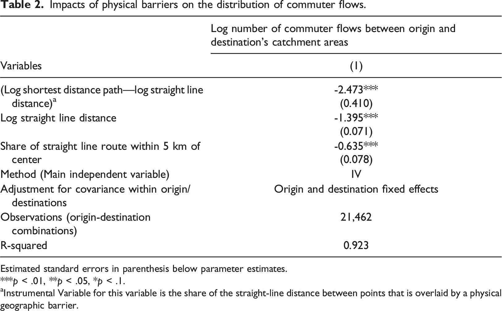
Estimated standard errors in parenthesis below parameter estimates.

***p < .01, **p < .05, *p < .1.

^aInstrumental Variable for this variable is the share of the straight-line distance between points that is overlaid by a physical geographic barrier.

The regression focuses on work trips only. We expect other types of travel—to schools, shopping and services, visits to friends—to also be negatively affected by increasing detours. Thus, the results probably underestimate the total impact of impeding barriers on travel between locations.

In conclusion, two points separated by physical barriers tend to have less commuting flows than expected, even if the same origin and destination generate substantial traffic into other—unimpeded—directions. Note that the reduction in the volume of trips between “obstructed” destinations cannot but partially ameliorate the impact of barriers on traffic congestion. Therefore, Table 2 suggests that the results in Table 1 are likely downward biased—that is, conservative—with respect to a structural model that conditioned on effective traffic volumes between locales.

Traffic and congestion diffusion in areas adjacent to barriers

We finally hypothesize that coastal trips may be subject to a higher probability of congestion, even when they happen between points that are not obstructed by natural barriers—as in trips that occur along a straight line running in parallel to the coast. During peak hours, the duration and degree of congestion in specific roads are partially determined by their ability to diffuse traffic flows. Drivers are more likely to take alternative roads when the shortest path is congested. The mileage of the STP will tend to grow relative to the SDP in congested time periods or road segments. Although the distribution of roads is sometimes modeled as approximately ring-radial or gridded (Chen et al., 2015), geographic features often constrain opportunities for alternative routing. We therefore hypothesize that the chances of finding nearby uncongested substitute routes will determine the ability of the local road network to diffuse sudden commuter flows.

Local traffic diffusion can be thought of as akin to heat conduction (Helbing. 2001; Jordan, 2005). Assume the existence of a number of workers in a semicircular segment at distance R of the city center (Figure 3) making decisions about how to commute to the core (point C). Point A is adjacent to the coast, whereas B is far inland. For simplicity, assume that commuters first choose to drive in parallel—that is, not getting closer to their destination—to a point along the semicircular segment, and then irreversibly drive in a straight line (e.g., dash lines in Figure 3) toward the center. Note that—by assumption—the commute from A to C is not directly impeded by any barrier.

Figure 3.

Commutes to the center from a semicircular segment at distance R. A and B represent two commuting origins. A is adjacent to the coast, whereas B is far inland. We assume that commuters originating from A and B would like to find a less congested path—faster than the SDP—to commute to C. We name the—arbitrarily chosen—points where they can find these fastest paths “optimal points.” Commuters from B have better access to both of them. As exposited in the text, the ability of point A to diffuse congestion is constrained by the coast.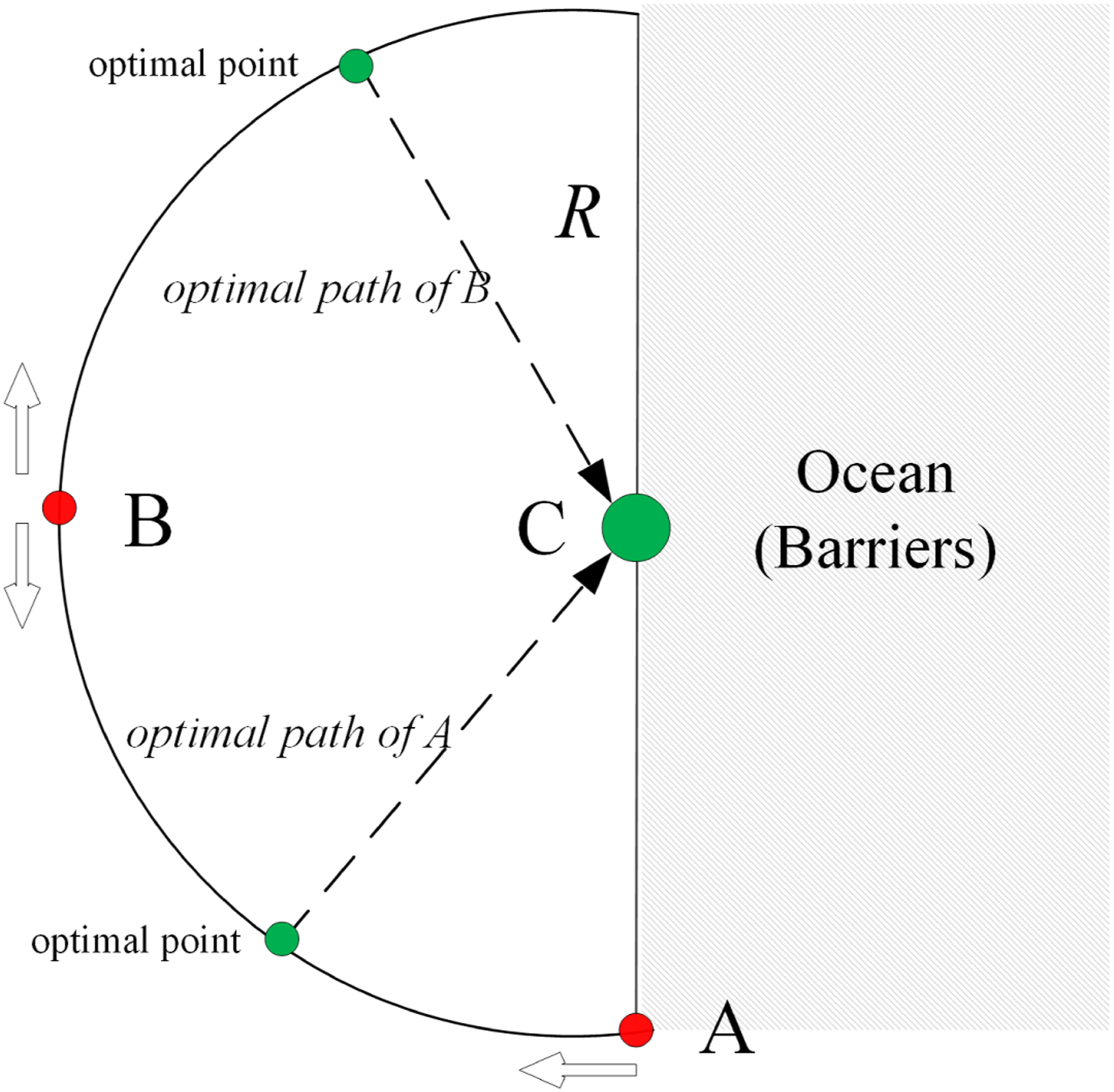

If the straight line path between a point and the center has more traffic than other proximate locations along the semi-circle, some commuters will bypass the SDP, driving along the semi-circle to find a less congested route. Route-shopping commuters’ STD mileages will be bigger than the corresponding SDPs. However, they must be saving time overall. In addition, by leaving congested points, they will relief traffic pressures in these, but increase them in adjacent areas. Hence, traffic flows diffuse from congested areas into proximate, less-transited ones.

As in heat diffusion models (Appendix. Heat equation model), the semicircular line segment is analog to a one-dimensional “rod” with length L. The initial temperature or traffic congestion—for example, the negative of the average speed of trips from each point to the center in $L$ km/hour—along the entire rod is $T_{1}$ . The boundaries are fully insulated, with no heat (traffic) transmission possible from the ends of the segment into the ocean $\frac{δ T (0)}{δ x} = \frac{δ T (l)}{δ x} = 0$ . We assume that congestion always diffuses from slower to faster adjacent points.

Consider now the possibility of a single place $(x = 1)$ being subject to a sudden convective heat transfer at time 0—in our analog a traffic surge, implying slower commutes to the center. In theory—as commuters effect a sequence of lateral moves from the direction of $l$ to avoid congestion—the rod will reach the steady-state “temperature” (congestion) $T_{2}$ at time $Τ$ . Derived from Fourier’s law (Baron Fourier, 1878), the quantity of transferred heat will be the same regardless of the location of the heat input. However, the duration of the heat diffusion process $(Τ)$ will vary: concentrated congestion surges are more likely to be sustained in points closer to the end of segment—in coastal areas.

The duration time for full diffusion τ is a function of the characteristic length l_c, which ranges between L/2 and L. From Figure 4, the optimal characteristics length is L/2—with duration time $(T_{1})$ being smaller than the time under the longest characteristic length $(T_{2})$ .

Figure 4.

The heat conduction process of an insulated even rod. At time 0, a sudden external heat is transferred to point x (Panel A). Consequently, heat conduction will continue until the extra heat at point x diffuses throughout, and the rod reaches a new steady-state at time τ. Under reasonable assumptions, the relationship between heat conduction duration and the location of the heating point is linear from 0−L/2 to L/2−L (Panel B). τ is at its smallest when the heating inflow point is at the middle of the rod. Similarly, compare sudden external commuter flows to the middle and extreme points of a semicircle around the destination (Panel C). A longer time is required for full diffusion from the extreme points.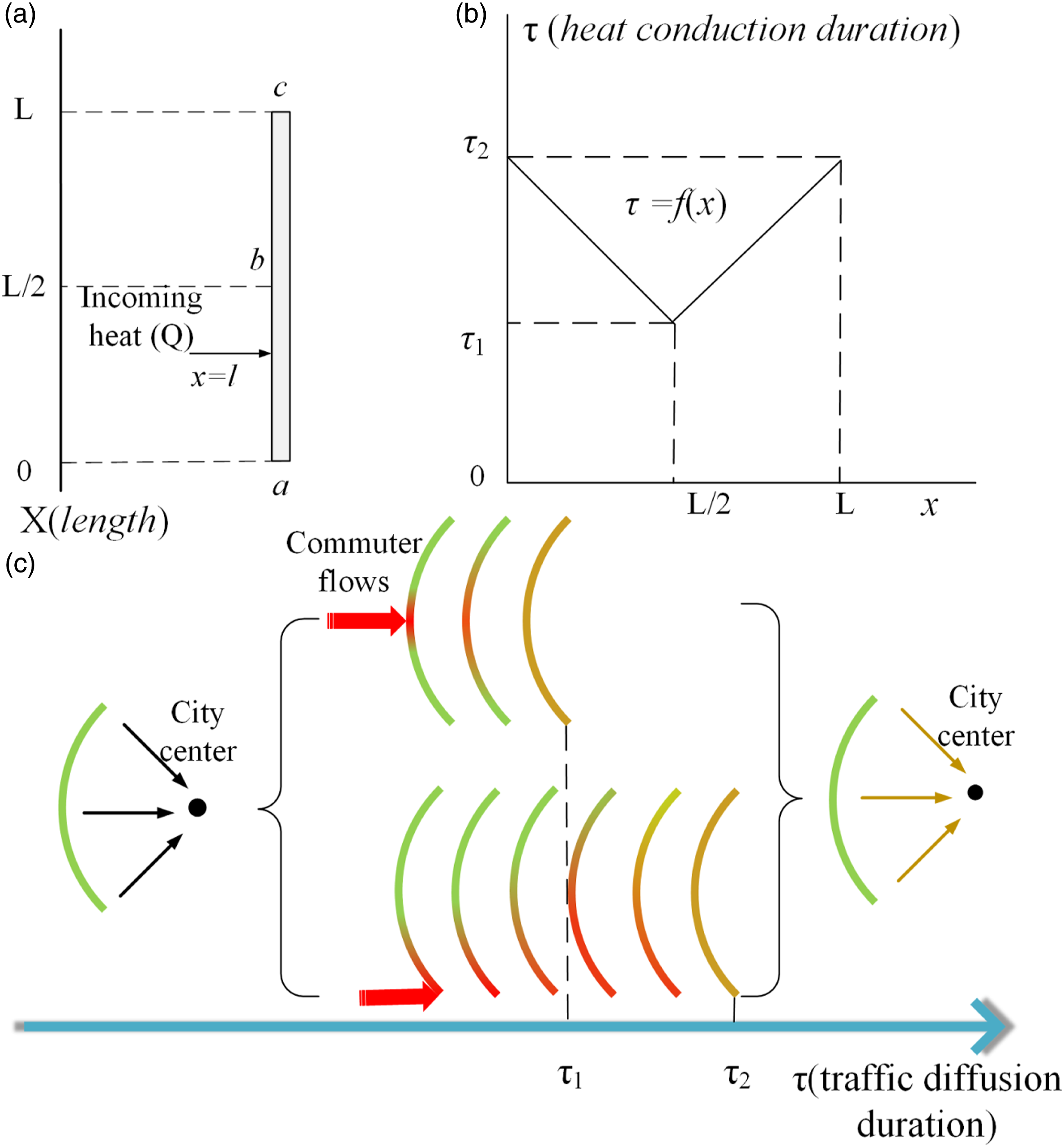

The intuition for the result is simple. In the middle of the segment, heat—congestion—diffuses in both directions with least impedance. In areas closer to the end of the rod diffusion ends quickly on one side—as temperatures between the surge and the closest boundary point equalize. Thereafter diffusion happens—with reflux—solely in the direction opposite to the closest boundary. In fact, for some time, the maximum level of congestion will be at the boundary. Another analog is provided by the diffusion of pollutants. Cushman-Roisin (2012) notes that “naturally, it takes longer to spread something when it first comes from one extremity than when it originates at the center.”

Hence, surges of traffic along coastal routes may experience longer times diffusing, because the ocean partially impedes the ability of drivers to bypass congestion. This implies that driving times could be longer in coastal routes at peak times, and that the difference between congested and uncongested driving times should be larger for trips running close to geographical barriers.⁶

We test these hypotheses in Table 3. For consistency with previous specifications, we start using the share of the SLD that is transected by barriers as a first proxy for coastal routes. The higher the measure, the more likely that the straight segment between points “hits” the coast earlier on. A second—and more direct—measure is the share of the SDP track that lies within 5 km of the ocean. We focus our discussion on this independent variable.

Table 3.

Impacts of physical barriers on congestion diffusion in areas adjacent to barriers.

Variables	Log Google maps driving time at 8 a.m.		(Log Google maps driving time at 8 a.m.)-(Log Google maps driving time daily average)
Variables	(1)	(2)	(3)	(4)
Share of SLD impeded by geographic barrier	0.080***		0.298***
	(0.010)		(0.008)
Share of the SDP track within 5 km of the ocean		0.114***		0.042***
		(0.006)		(0.005)
Log shortest distance path	0.867*** (0.002)	0.862*** (0.002)	0.144*** (0.001)	0.149*** (0.001)
Share of straight line route within 5 km of center	-0.0207***	-0.046***	-0.015***	-0.009*
	(0.006)	(0.006)	(0.004)	(0.005)
Adjustment for covariance within Origin/Destinations		Origin and destination fixed effects
R-squared	0.932	0.933	0.777	0.761
Observations (origin-destination combinations)			21,462

Standard errors in parentheses below parameter estimates.

***p < .01, **p < .05, *p < .1.

Columns 1 and 2 in Table 3 follow equation (4) with fixed effects. We start with the study the impact of coastal routes on the log of driving time at peak traffic (8 a.m.). Importantly, we now control for the log of the SDP on the right-hand side. Results clearly demonstrate that coastal trips are slower in this environment. For instance, in column 2 of Table 3, if the coastal share of the SDP route increased from 0 to 50%, the same trip would take a 5.7% longer time.

We next subtract the log of Google maps’ driving average commuting time from the 8 a.m. peak, and use the resulting measurement as a new dependent variable. How do commutes during peak time differ from regular ones? According to the logic of the heat equation, surges in traffic should be associated with worse outcomes in the routes that are constrained by geography. This is indeed what we find in column 4 of Table 3: coastal routes display longer peak-time extra delays than inland ones. For instance, a 50% increase in the share of the SDP that runs close to the ocean implies a trip that is 2.1% longer at 8 a.m. than it is on average during the day.

Conclusions

Scientists are increasingly studying the impacts of city shapes on social and environmental urban outcomes (Amindarbari and Sevtsuk, 2012; Angel and Franco, 2018; Angel et al., 2010; Batty, 2008; Harari, 2020; Newton, 2000). Current urban shape, density, and function are typically explained as products of city planning, land use, transportation infrastructures, social trends, and economic factors. Focusing on vehicular traffic congestion, we show a large quantitative role for physical geography, especially salient in areas where the “downtown” or commercial center is near the ocean or mountains. According to 2010 Census data, 39% of the U.S. population lived within a few miles of the coast (Crossett et al., 2014).

We gathered data about commuting intensity, road distances, topography, and driving outcomes for 21,462 trips between geographically representative points in the Boston metropolitan area. We documented and found supporting evidence for four separate impacts of geographic barriers on commuting patterns.

Effect #1: geographic barriers lead to longer driving distances and commuting times wherever they generate substantial non-convexities in the urban form. While obvious, we provide a simple approach to quantify this phenomenon at the level of each potential trip.

Effect #2: geographic barriers can divert traffic into the city center, making downtown trips slower and decreasing the efficiency of the whole transportation system. In the case of Boston—using actual commuting flows—we estimate that 13.73% of the traffic in the city center is derived from trips that have to bypass the ocean through the urban core. These trips would have gone through lateral—less-congested—routes in a regularly shaped city. This pattern is likely to arise in other cities that expanded around a harbor, which tends to be at the vertex of a natural bay—with the ocean bulging into the land.

Effect #3—likely due to the two previous effects—the existence of barriers between two points reduces commuter flows between them, as we confirm empirically. These missing trips must be occurring somewhere else. If the costs of congestion are nonlinear in the amount of traffic, this effect might prevent the distribution of trips to even out, likely harming overall commuting outcomes.

Effect #4: trips that have to go nearby barriers are more prone to localized congestion peaks. As in heat conduction or pollutant-spill diffusion processes, the ability of the road system to diffuse sudden traffic inflows or the impact of incidents is reduced in areas that are adjacent to barriers.

These four effects—as shown in this paper—are generally combined with effect #5—as exposited in (Saiz 2010): by reducing the amount of buildable land, physical barriers tend to push away real estate development at further distances from the downtown, lengthening commuting distances to the city’s edge. In geographically constrained regions, high-density redevelopment of central areas could mute such pressures. However, this requires substantial housing price appreciation there to make economic sense, exacerbating affordability issues.

Bridges and tunnels can sometimes provide relief to the problems illustrated in the paper, but they cannot be feasibly built everywhere—be it by engineering or economic limitations. In addition, they tend to quickly get congested themselves. Boston provides an interesting case study, as its largest and most controversial highway investment—the Big Dig, deriving the city’s coastal highways into subterranean tunnels—is arguably related to congestion arising from the natural constraints surrounding its downtown area. Yet despite these tunnels, we still find large negative impacts of coastal barriers on local traffic.

Beyond building tunnels and bridges, transportation planners should devote extraordinary attention to the areas where natural barriers generate congestion. An explicit policy objective should be to avoid cities becoming too disconnected. Policymakers should perhaps allow for additional system redundancies to service naturally constrained locales. For instance, massive public transport investments may make more sense in locations with low traffic-diffusion ability. Because of the high real estate value of coastal land, transportation system redundancies might be feasibly built slightly inland, in parallel to the coast.

In rapidly growing economies—where cities and large master-planned communities are being designed and built ex novo—it seems sensible to be cautious about planning new downtowns close to large natural barriers. New housing development is attractive and desirable there—due to the amenity effects of proximity to water or hills. Nevertheless, one could consider situating office or industrial development a bit away from oceans or lakes, with transportation systems connecting coastal homes to inland jobs in directions that are perpendicular to the barriers.

In addition, the results show that one has to be careful when comparing the environmental and social outcomes of urban transportation systems across cities. Before assigning specific weights to differences in human behavior or policies, one must take into account the different configuration of physical barriers across urban environments.

Footnotes

Acknowledgments

We would like to thank Zehua Ma (Xi’an Jiaotong University) for his advice in using heat equation model.

Declaration of conflicting interests

The author(s) declared no potential conflicts of interest with respect to the research, authorship, and/or publication of this article.

Funding

The author(s) received no financial support for the research, authorship, and/or publication of this article.

Data and materials availability

All data are available in the main text or the Appendix.

Notes

Appendix

References

Ahlfeldt

McMillen

(2018) Tall buildings and land values: height and construction cost elasticities in Chicago, 1870–2010. Review of Economics and Statistics 100(5): 861–875.

Akbar

(2021) The fast, the slow, and the congested: Urban transportation in rich and poor countries. Tech. Rep.

Akbar

Duranton

(2017) Measuring the Cost of Congestion in Highly Congested City: Bogotá. Buenos Aires: Tech. Rep. CAF Development Bank Of Latinamerica.

Akbar

Couture

Duranton

, et al. (2018) Mobility and Congestion in Urban India. Geneva, Switzerland: The World Bank.

Amindarbari

Sevtsuk

(2012) Measuring growth and change in metropolitan form. Sciences 104(17): 7301–7306.

Anderson

Rubin

(1949) Estimation of the parameters of a single equation in a complete system of stochastic equations. The Annals of Mathematical Statistics 20(1): 46–63.

Angel

Franco

. The shape compactness of urban extents. Working paper: Lincoln Institute of Land Policy working paper (2018).

Angel

Parent

Civco

(2010) Ten compactness properties of circles: measuring shape in geography. The Canadian Geographer/Le Géographe Canadien 54(4): 441–461.

Angrist

GuidoImbens

Rubin

(1996) Identification of causal effects using instrumental variables. Journal of the American statistical Association 91(434): 444–455.

10.

Arnott

De Palma

Lindsey

(1992) Route choice with heterogeneous drivers and group-specific congestion costs. Regional Science and Urban Economics 22(1): 71–102.

11.

Baron Fourier

JBJ

(1878) The Analytical Theory of Heat. Oxford, UK: The University Press.

12.

Batty

(2008) The size, scale, and shape of cities. Science 319(5864): 769–771.

13.

Black

Paez

Suthanaya

(2002) Sustainable urban transportation: performance indicators and some analytical approaches. Journal of Urban Planning and Development 128(4): 184–209.

14.

Boarnet

Crane

(2001) The influence of land use on travel behavior: spec- ification and estimation strategies. Transportation Research Part A: Policy and Practice 35(9): 823–845.

15.

Carruthers

Ulfarsson

(2003) Urban sprawl and the cost of public ser- vices. Environment and Planning B: Planning and Design 30(4): 503–522.

16.

Cengel

Ghajar

(2014) Transient heat conduction. In: Heat and Mass Transfer: Fun- Damentals and Applications. New York, NY: McGraw-Hill Education.

17.

Cervero

(1989) Jobs-housing balancing and regional mobility. Journal of the American Planning Association 55(2): 136–150.

18.

Chapman

(2007) Transport and climate change: a review. Journal of Transport Geography 15(5): 354–367.

19.

Chen

Cassidy

, et al. (2015) Optimal transit service atop ring-radial and grid street networks: A con- tinuum approximation design method and comparisons. Transportation Research Part B: Methodological 81: 755–774.

20.

Cole

King

CAM

(1968) Quantitative Geography: Techniques and Theories in Geography. New York: Wiley.

21.

Crossett

Ache

Pacheco

Haber

(2014) National Coastal Population Report, Population Trends from 1970 to 2020. Washington, DC: NOAA State of the Coast Report Series, US Department of Commerce.

22.

Cushman-Roisin

(2012) Environmental Transport and Fate. Hanover, NH: Thayer School of Engineering Dartmouth College, University Lecture, 2.

23.

De Vlieger

De Keukeleere

Kretzschmar

(2000) Environmental effects of driving behaviour and congestion related to passenger cars. Atmospheric Environment 3427: 4649–4655.

24.

Dunphy

Fisher

(1996) Transportation, congestion, and density: new in- sights. Transportation Research Record 1552(1): 89–96.

25.

Duque

Lozano-Gracia

Patino

, et al. (2019) Urban Form and Productivity: What Is the Shape of Latin American Cities? Geneva, Switzerland: The World Bank.

26.

Figliozzi

(2011) The impacts of congestion on time-definitive urban freight distri- bution networks CO2 emission levels: Results from a case study in Portland, Oregon. Transportation Research Part C: Emerging Technologies 19(5): 766–778.

27.

Ganin

Kitsak

Marchese

, et al. (2017) Resilience and efficiency in transportation networks. Science Advances 3(12): e1701079.

28.

Giuliano

(1995) The weakening transportation-land use connection. Access Maga- Zine 1(6): 3–11.

29.

Giuliano

Small

(1993) Is the journey to work explained by urban structure? Urban Studies 30(9): 1485–1500.

30.

Green

Hogarth

Shackleton

(1999) Longer distance commuting as a substitute for migration in Britain: a review of trends, issues and implications. International Journal of Population Geography 5(1): 49–67.

31.

Hamilton

(1989) Wasteful commuting again. Journal of Political Economy 97(6): 1497–1504.

32.

Hamilton

Röell

(1982) Wasteful commuting. Journal of Political Economy 90(5): 1035–1053.

33.

Hanson

Pratt

(1988) Reconceptualizing the links between home and work in urban geography. Economic geography 64(4): 299–321.

34.

Hansson

Mattisson

Bjork

, et al. (2011) Relationship between commuting and health outcomes in a cross- sectional population survey in southern Sweden. BMC Public Health 11(1): 834.

35.

Harari

(2020) Cities in bad shape: urban geometry in India. American Economic Review 110(8): 2377–2421.

36.

Chow

C-Y

Zhang

J-D

. A comparative analysis of journey time from Google maps and intelligent transport system in Hong Kong. In: 2019 IEEE 21st International Conference on High Performance Computing and Communications; IEEE 17th International Conference on Smart City; IEEE 5th International Conference on Data Science and Systems (HPCC/SmartCity/DSS), 10–12 August 2019. 2019, pp. 2610–2617. doi: 10.1109/HPCC/SmartCity/DSS.2019.00366

37.

Helbing

(2001) Traffic and related self-driven many-particle systems. Reviews of modern physics 73(4): 1067–1141.

38.

Hensen

De Vries

Cörvers

(2009) The role of geographic mobility in reducing education-job mismatches in the Netherlands. Papers in Regional Science 88(3): 667–682.

39.

Horner

(2004) Spatial dimensions of urban commuting: a review of major issues and their implications for future geographic research. The Professional Geographer 56(2): 160–173.

40.

Huang

Levinson

Wang

, et al. (2018) Tracking job and housing dynamics with smartcard data. Proceedings of the National Academy of Sciences 115(50): 12710–12715.

41.

Incropera

Lavine

Dewitt

, et al. (2007) Fundamentals of Heat and Mass Transfer. Hoboken, NJ: Wiley.

42.

Jordan

(2005) Growth and decay of shock and acceleration waves in a traffic flow model with relaxation. Physica D: Nonlinear Phenomena 207(3–4): 220–229.

43.

Kleibergen

Paap

(2006) Generalized reduced rank tests using the singular value decomposition. Journal of Econometrics 133(1): 97–126.

44.

Krizek

Power

(1996) A planners guide to sustainable development. Tech. Rep.

45.

Leape

(2006) The London congestion charge. Journal of Economic Perspectives 20(4): 157–176.

46.

Walker

Srinivasan

, et al. (2010) Modeling private car ownership in China: investigation of urban form impact across megacities. Transportation Research Record: Journal of the Transportation Research Board, Transportation Research Record 2193(1): 76–84.

47.

Lucy

Phillips

(1997) The post-suburban era comes to Richmond: city decline, suburban transition, and exurban growth. Landscape and Urban Planning 36(4): 259–275.

48.

K-R

Banister

(2006) Excess commuting: a critical review. Transport Reviews 26(6): 749–767.

49.

Massaro

Ganin

Perra

, et al. (2018) Resilience management during large-scale epidemic outbreaks. Scientific Reports 8(1): 1–9.

50.

McGovern

(1998) Controlling the environmental impact of transport: traffic management schemes and their influence on consumer behaviour. Sustainable Development 6(1): 23–30.

51.

Miranda

(2020) The shape of segregation: the role of urban form in immigrant assimilation. Cities 106: 102852.

52.

Morawska

Ristovski

Jayaratne

, et al. (2008) Ambient nano and ultrafine particles from motor vehicle emissions: characteristics, ambient processing and implications on human exposure. Atmo- spheric Environment 42(35): 8113–8138.

53.

Newton

(2000) Urban form and environmental performance. Achieving Sustainable Urban Form 2: 46–53.

54.

O’Regan

Quigley

(1998) Accessibility and economic opportunity. Available at SSRN 131308 working paper.

55.

Prato

Bekhor

(2006) Applying branch-and-bound technique to route choice set generation. Transportation Research Record 1985(1): 19–28.

56.

Rietveld

Piet

Zwart

van Wee

, et al. (1999) On the relationship between travel time and travel distance of com- muters. The Annals of Regional Science 33(3): 269–287.

57.

Rolheiser

Dai

(2019) Beyond density: municipal expenditures and the shape and location of development. Urban Geography 40(8): 1097–1123.

58.

Saiz

(2010) The geographic determinants of housing supply. The Quarterly Journal of Economics 125(3): 1253–1296.

59.

Scott

PavlosKanaroglou

Anderson

(1997) Impacts of commuting efficiency on congestion and emissions: case of the Hamilton CMA, Canada. Trans- Portation Research Part D: Transport and Environment 2(4): 245–257.

60.

Stock

Yogo

. Testing for Weak Instruments in Linear IV Regression. In: Andrews

DWK

(ed) Identification and Inference for Econometric Models. New York, NY: Cambridge University Press, 2005, 80–108.

61.

Stokes

Seto

(2018) Tradeoffs in environmental and equity gains from job accessibility. Proceedings of the National Academy of Sciences 115(42): E9773–E9781.

62.

Sultana

(2002) Job/housing imbalance and commuting time in the Atlanta metropolitan area: exploration of causes of longer commuting time. Urban Geography 23(8): 728–749.

63.

Sultana

(2000) Some effects of employment centers on commuting times in the Atlanta metropolitan area, 1990 Southeastern Geographer 40(2): 225–233.

64.

Tang

Levinson

(2018) Deviation between actual and shortest travel time paths for commuters. Journal of Transportation Engineering, Part A: Systems 144(8): 04018042.

65.

Taylor

Ong

(1995) Spatial mismatch or automobile mismatch? An exami- nation of race, residence and commuting in US metropolitan areas. Urban Studies 32(9): 1453–1473.

66.

Van Ommeren

Dargay

(2006) The optimal choice of commuting speed: consequences for commuting time, distance and costs. Journal of Transport Economics and Policy (JTEP) 40(2): 279–296.

67.

Wang

Djahel

Zhang

, et al. (2016) Next road rerouting: a multiagent system for mitigating unexpected urban traffic congestion. IEEE Transactions on Intelligent Transportation Systems 17(10): 2888–2899.

68.

Wheaton

(2004) Commuting, congestion, and employment dispersal in cities with mixed land use. Journal of Urban Economics 55(3): 417–438.

69.

White

(1986) Sex differences in urban commuting patterns. The American Economic Review 76(2): 368–372.

70.

Zegras

(2010) The built environment and motor vehicle ownership and use: evidence from Santiago de Chile. Urban Studies 47(8): 1793–1817.

71.

Zhang

Malczewski

(2019) Quality evaluation of volunteered geographic in- formation: The case of OpenStreetMap. In: Crowdsourcing: Concepts, Methodologies, Tools, and Applications. Pennsylvania, PA: IGI Global, pp. 1173–1201.

72.

Zhang

Zeng

, et al. (2019) Scale-free resilience of real traffic jams. Proceedings of the National Academy of Sciences 116(18): 8673–8678.

73.

Zhou

Murphy

Corcoran

(2019) Integrating road carrying capacity and traffic congestion into the excess commuting framework: the case of Los Ange- les. Environment and Planning B: Urban Analytics and City Science 47(1): 119–137.

74.

Zhu

Levinson

(2015) Do people use the shortest path? An empirical test of Wardrop’s first principle. Plos One 10(8).

Physical geography and traffic delays: Evidence from a major coastal city

Abstract

Keywords

Introduction

Data and methods

Data

Empirical methods

Effect of geographical barriers on commuting outcomes and downtown congestion

The effect of physical barriers on the distribution of commuter flows

Traffic and congestion diffusion in areas adjacent to barriers

Conclusions

Footnotes

Acknowledgments

Declaration of conflicting interests

Funding

Data and materials availability

Notes

Appendix

References