
Abstract
Exploring the nature of spatial and temporal variation in house prices is important because it can help better understand such issues as affordability and equity of access to housing. In the UK, research on house price variation has been hindered by a lack of extensive data linking the prices of properties at different places and times to their physical attributes. This paper addresses this gap through using a new dataset linking Land Registry Price Paid Data to attribute data from Ordnance Survey and Energy Performance Certificates datasets. The new data are used to investigate spatial disparities in England’s house prices at four geographical scales (from local authority to individual address) between 2009 and 2016 – a period of sustained price rises after the global financial crisis of 2008. We selected two housing price measures for comparison, namely transaction price and the house price per square metre. Multilevel variance components models are used to estimate variation in the two house price measures at four different spatial scales and we compare spatial disparities in the two measures at these different scales. Our results suggest that accounting for the size of properties by using house price per square metre offers a more accurate picture of house price variation than does the use of transaction prices at the same geographic scale. Spatial disparities in house price per square metre are more apparent and are seen to be clustered at local authority level and highly clustered at Middle Layer Super Output Area level, with imbalances increasing during this eight-year period and highlighting the strong and growing influence of London on the national housing market.
Introduction
Shelter is a basic human need, but a majority of countries now face critical housing challenges (UN-HABITAT, 2011a, 2011b, 2012). In wealthier countries such as the UK, residential property prices, on the whole, have been rising since the mid-1990s (Knoll et al., 2017), but prices can exhibit huge sub-national geographic variations (Fotheringham et al., 1998; Huang et al., 2010). In the UK, prices in London can be prohibitively high, whereas in the de-industrialised North, properties have occasionally been purchased for a few pounds (Edwards, 2016; Nsubuga, 2018). These variations can be understood through examining published house price statistics (the term ‘house price’ is frequently used in relation to all types of residential property). These have been reported in Britain for a long time but local heterogeneity in stock composition, sales frequency and transaction volumes means that data analysis can be challenging, particularly when focusing on small area geographies. Transaction prices (TPs) are frequently reported at regional or city level in order to smooth out some of this variation. Different organisations produce these statistics using different measurement methods and datasets (Chandler and Disney, 2014; Wood, 2015). The Nationwide Building Society (2015) produces a regional quarterly house price index with its mortgage lending data while the Office for National Statistics (ONS) publishes a regional house price index (ONS et al., 2016) based on Land Registry data. Both datasets are published at regional level, but they are not comparable due to differences in data definition and the housing characteristics considered when using the ‘mix-adjusted’ approach. Lack of comparability can present difficulties when researching house price variation (Gray, 2012; Hamnett and Reades, 2019).
Despite data challenges, quantitative analyses of house price variation at multiple geographic scales have been conducted within individual cities in the UK, such as London (Feng and Jones, 2016; Law, 2018) and Cardiff (Orford, 2002; Wang et al., 2015). In three of these four papers, TP variation was explored (Feng and Jones, 2016; Orford, 2002; Wang et al., 2015) using the Land Registry Price Paid Data (PPD). The local variations in stock composition and other factors mean that simple aggregation for the purposes of studying price variations is problematic. One suggested solution has been to examine house price patterns using house price per square metre (HPM), but to date, only Powell-Smith (2017) has achieved this with any degree of success.
Systematic analyses of house price variation at a variety of geographic scales and accounting for the local variations in stock characteristics could better aid both government and public in understanding housing inequalities in England. This research takes a first step by modelling the patterns of house price variation across England at multiple geographical scales while taking into account local variations in total floor area. House price variation in terms of both TP and HPM is explored utilising a new dataset which links entries in the Land Registry PPD to building locations from Ordnance Survey datasets and total floor area from the Domestic Energy Performance Certificates (EPCs) dataset (Chi et al., 2019). In this paper, we first demonstrate the utility of this new linked dataset, and then explore how the factors that affect house prices can operate at different spatial scales. Accounting for variations in individual property characteristics (i.e. total floor area) permits these spatial effects to be revealed. The second section reviews relevant literature on the spatial dimension of house price variation. Our study area and data are introduced in the third section. The fourth section presents the concept of multilevel variance components models and defines 16 multilevel models (two types of model applied to eight yearly datasets) used in this research. The fifth section presents and discusses the results. Finally, conclusions and recommendations for future research are provided.
The spatial dimension of house price variation
House prices are spatially auto-correlated in small areas but also spatially heterogeneous in different geographical locations (Basu and Thibodeau, 1998; Goodman and Thibodeau, 2003). Research shows the drivers behind house price variation are complex and operate at different geographical scales in England (Cook, 2005; MacDonald and Taylor, 1993; Szumilo et al., 2017; Yao and Fotheringham, 2016). At the broadest national or regional scales, house prices are influenced by macro-structural political, economic and demographic factors (Ferrari and Rae, 2013; Meen, 1999), such as regional economic development, infrastructure provision and policies affecting migration. At a scale that might include cities, local authorities (LAs) or travel-to-work areas, house prices are influenced by urban form, local economic conditions and amenities, and the availability of different transport modes (Downes, 2018; Smith, 2018). At extended neighbourhood scales, house prices are influenced by local amenities, the character of neighbouring households, local public goods (i.e. schools and open space) and the availability of public transport (Orford, 2002). House prices along the same street or in a local neighbourhood tend to be similar to each other, but may vary as a result of physical qualities such as dwelling size, age, structural design and historic value (Ahlfeldt et al., 2012; Goodman and Thibodeau, 1995; Kain and Quigley, 1970).
Various modelling techniques have been proposed to capture spatial heterogeneity in property prices over a large area, such as traditional regression-based hedonic price models (Visser et al., 2008), geographically weighted hedonic regression models (Helbich et al., 2014; Lu et al., 2014; Yu, 2007), geographically and temporally weighted regression models (Fotheringham et al., 2015; Huang et al., 2010) and multilevel models (Jones and Bullen, 1993, 1994). Jones (1991) first applied multilevel models to analyse house price variation showing that they demonstrate a considerable improvement over the traditional linear hedonic price modelling. Subsequent research using multilevel models has explored house price variation across the world (Dong et al., 2015; Goodman and Thibodeau, 1998; Leishman, 2009). Orford (2002) applied multilevel modelling to estimate the effects of location upon Cardiff house prices suggesting that the overall house price variation is composed of variation within districts, within communities and across individual properties. Recently, Feng and Jones (2016) were the first to present London’s house price variation at five geographical scales determined by postcode and census geography. These two geographical classifications showed that TP was hierarchical and highly clustered at smaller geographical scales.
Current research suggests house price variations can occur across geographies but may also vary with house characteristics. Aggregate statistics for house prices at a large geographical scale will mask variation at smaller scales. Moreover, most previous hedonic analyses are applied to regional level or single city examples. A framework that integrates housing market analyses in England at different spatial scales does not currently exist. This suggests an incomplete understanding of the spatial determinants of the variations in Britain’s housing market.
Study area and data
Study area and geographical scales
The study area is England, which is comprised of a nested hierarchy of spatial units. While there are many possible units that England could be broken down into, here we have chosen 9 Regions, 326 LAs, 6791 Middle Layer Super Output Areas (MSOAs) and 32,844 Lower Layer Super Output Areas (LSOAs) which have nested coterminous boundaries. The North East, the North West, Yorkshire and the Humber, East Midlands, West Midlands, East of England, the South East, the South West and London are the nine regions in England. Below this level, LAs may be the size of a county (e.g. Wiltshire) or town (e.g. Stroud). MSOAs and LSOAs were designed as statistical geographies for census outputs. MSOAs are larger, containing between 5000 and 15,000 residents and can often comprise areas that many think of as an extended neighbourhood. LSOAs are smaller, containing 1000–3000 residents (ONS, 2019) and may comprise a few streets in an urban area or what some may think of as a local neighbourhood. England’s house prices are frequently aggregated at regional, LA, MSOA and LSOA levels. Regional level house prices have been well explored (Cook and Watson, 2016; MacDonald and Taylor, 1993), few studies have explored house price variance at the lower, more detailed, geographic levels. Thus, this research considers three lower geographic levels (from LA to LSOA) plus the individual address level.
House price data
The Land Registry PPD is an open administrative dataset from Her Majesty’s Land Registry, first released in 2013. It is a register of residential property sales containing most property transactions, but excludes seven sale types such as those conducted under the government’s ‘right-to-buy’ scheme (HM Land Registry, 2016, 2020). It provides the most accurate picture of full market sale prices in the UK residential housing market (Marsden, 2015) but contains only a limited set of other attributes about each property. This is a barrier to the analysis of house price variance, because attributes such as property size are important determinants of price (De Nadai and Lepri, 2018; Orford, 2010). Thus, this paper uses a new linked dataset1 combining the Land Registry PPD with Domestic EPC data containing information on the total floor area (Chi et al., 2019). This enables house price variance analysis in terms of TP both normalised and non-normalised by floor area. The new linked dataset contains 4,682,468 transactions that occurred between 2009 and 2016, representing 80% of the full market housing sales in the Land Registry PPD over this period. Seven fields of this dataset are used in this research, namely TP, HPM, year of transaction, region codes, the 2011 Census LSOA codes, MSOA codes and LA district codes. HPM is calculated by using TP divided by the property’s total floor area. Supplementary material A reveals only a weak covariance relationship between TP and HPM in 2009. This indicates that TP and HPM do provide independent information on property prices, suggesting that we are justified in exploring both in this paper.
Methodology
Multilevel variance components model
The multilevel variance components model is a statistical model without explanatory variables (Raudenbush and Bryk, 2002; Ren et al., 2013). In exploring house price variations, it simultaneously decomposes the total house price variance at and across different geographical scales, thus quantifying the extent of spatial effects on house prices. Properties can be viewed as being nested within different geographical jurisdictions. Given a house price dataset, which records transactions occurring within different LAs, a two-level variance components model could be formulated, in which level 1 is the property level and level 2 is LA level. This multilevel variance components model can be written as:
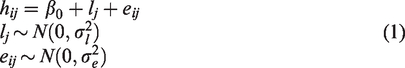
Here
Figure 1 offers a generic representation of equation (1) by illustrating house prices for 19 individual properties in two LAs (a and b). Individual house prices are shown as black circles, the overall mean house price (
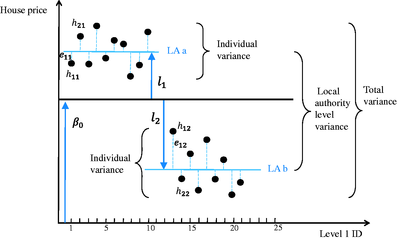
A graphical illustration of the two-level variance components model. LA: local authority.
The multilevel variance components model is decomposed by the overall mean house price (fixed effect) and the house price variation at each level (random effects). It treats the units at each level as a random sample from a larger population with an assumed distribution, decomposing the overall variance into two variance parts (
The two-level variance components model can be extended to three or more levels to examine the location effects at multiple scales simultaneously. Such an extension is straightforward, simply requiring the introduction of additional random effect terms. For example, a four-level model might have properties nested in LSOAs, then nested in MSOAs and then nested within LAs. This is written as:
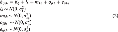
Here
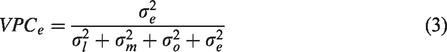
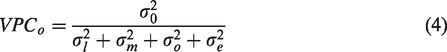
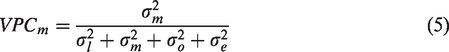
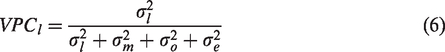
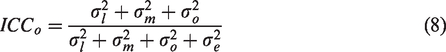
Variance partition coefficients (VPCs) can be used to interpret the variance components in a multilevel model. Taking the LA level as an example, the VPC of the LA level is calculated as the ratio of the LA variance to the total variance. It represents the proportion of the house price variance that can be attributed to differences between LAs. The VPC ranges from 0 to 1; 0 signifying no between-group differences and 1 signifying no within-group differences. A higher VPC at a particular level indicates larger differences between groups at that level. In the four-level variance components model, the total house price is decomposed into four variance components: individual level variance (
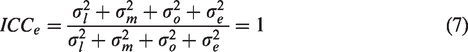
The intraclass correlation coefficient (ICC) offers another approach to interpreting the variance component. It measures the expected correlation (similarity) of observations within the same group at a particular level (Bartholomew et al., 2008). It is expressed as a ratio of variances, comparing the house price variance that is between groups at a particular level to the total variation (Finch and Bolin Je Kelley, 2014). In terms of ICC’s and VPC’s algebraic form, the ICC at any given level is the sum of the VPC at this level and all higher levels. For example, the ICC at the LA level is the same as its VPC, while at the MSOA level it is the sum of the MSOA and LA VPCs. The ICC ranges from 0 to 1, with higher values indicating a greater degree of clustering (meaning data are more similar within groups, with larger differences between groups). Equations for the ICC from individual level to LA level are shown in equations (7) to (10).
Exploring spatial influences on price variation
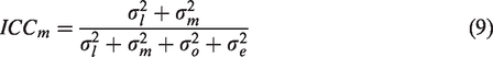
A four-level variance components model was used to estimate house price variance at the four levels of spatial aggregation. Level 1 is the individual residential property, level 2 is the LSOA level, level 3 is the MSOA level and level 4 is the LA level. Table 1 presents the 16 multilevel models used in this research and it applies two types of model (TP and HPM) to eight yearly datasets from 2009 to 2016.
The 16 candidate four-level variance component models. a
HPM: house price per square metre; TP: transaction price.
Note:
The model used in this research is based on TP and HPM; we do not take logarithms of prices, as is common practice across some of the literature, for the following reasons. First, the VPC pattern across the four levels is similar whether using house price or log house price as the output variable (Table B in supplementary material B). The conclusions of this research would therefore be the same under both methods. Second, when comparing the estimated mean price and observed mean price from the HPM model (i.e. HPM2009) with the log house price model, the two models show similar results and the estimated price in the HPM model shows a higher association with the observed mean (Figure B). Given these two reasons, this research uses the simpler and more easily interpreted model based on the unlogged price.
Results and discussion
Models presented in Table 1 were run using MLwiN 3.03 (Charlton et al., 2019). Likelihood ratio tests are used to establish whether the four-level variance components model fits the data significantly better than the null single-level model. Each four-level model in Table 1 is preferred to its null single-level model based on the near zero p-value of the likelihood ratio test. In addition, each four-level multilevel model was compared to a set of three-level models formed by dropping one geographic level for each comparison (e.g. dropping the LSOA level in the four-level model). All comparisons showed a significant increase in explanatory power with increasing numbers of levels according to the near zero p-values obtained from likelihood ratio tests. Hence the following discussions are based on the estimated coefficient values for the four-level variance component models in Table 1.
Overall house price change and house price variance
Following the financial crisis, both the estimated mean TP and mean HPM show the same increasing trend between 2009 and 2016 (Figure C1.A in supplementary material C). Overall house price variation increased between 2009 and 2016 (Figure C1.B in supplementary material C). The trend of house price variance differs depending on whether TP is normalised by the floor area of the property, henceforth we shall term the normalised TP as simply HPM. The variance of HPM increased between 2014 and 2015, while the variance of the TP decreased. Comparing the data in 2015 to 2014, a smaller number of full market value residential sales together with fewer sales at extremely high prices are the main reasons for the decrease in TP variance. This may be due to the increasing Stamp Duty Land Tax rates on higher bands at the end of 2014 limiting purchases of more expensive dwellings (Scanlon et al., 2017). One explanation for the trend discrepancy between TP and HPM is the different mix of stock sold in different years. For example, a higher proportion of large dwellings (total floor area bigger than 250 square metres) with high TPs (over £5 million) were sold in London’s housing market in 2014, but a lower proportion of these dwellings were sold in London in 2015 (Figure C2 in supplementary material C). Using the HPM approach, these large dwellings may have a low HPM; however, the small dwellings with high TPs may have a higher HPM. Therefore, the variance of HPM could increase. The overall TP variance is smaller than HPM variance. This not only means that normalised TPs by the floor area are more concentrated, but also that differences in total floor area contribute greatly to TP variance.
House price variance at four geographic scales
For both TP and HPM, VPC results reveal (Figure 2) that house price variance does exist between LAs, within-local-authority-between-MSOAs and also within-MSOA-between-LSOAs. HPM variance across different levels follows a similar pattern as TP variance, but with a higher variability at the same level. Comparing VPC at the same level and same year for HPM against TP reveals that once variations in property size are controlled for, spatial effects become much stronger. This reveals that controlling for floor area offsets much of the house price variation among individual properties and correspondingly increases VPC at higher geographic levels (i.e. level 4 to level 2). LA effects (compared to other spatial effects) had more of an influence on TPs in 2016 than in 2009, but when floor area is accounted for, this change in the LA’s influence is even more noticeable. Meanwhile, MSOA or LSOA effects are stable from 2009 to 2016. The conclusion drawn here is that the HPM aggregated at geographic level (i.e. LA level or MSOA level or LSOA level) offers a more accurate picture of the England’s housing market than TP.
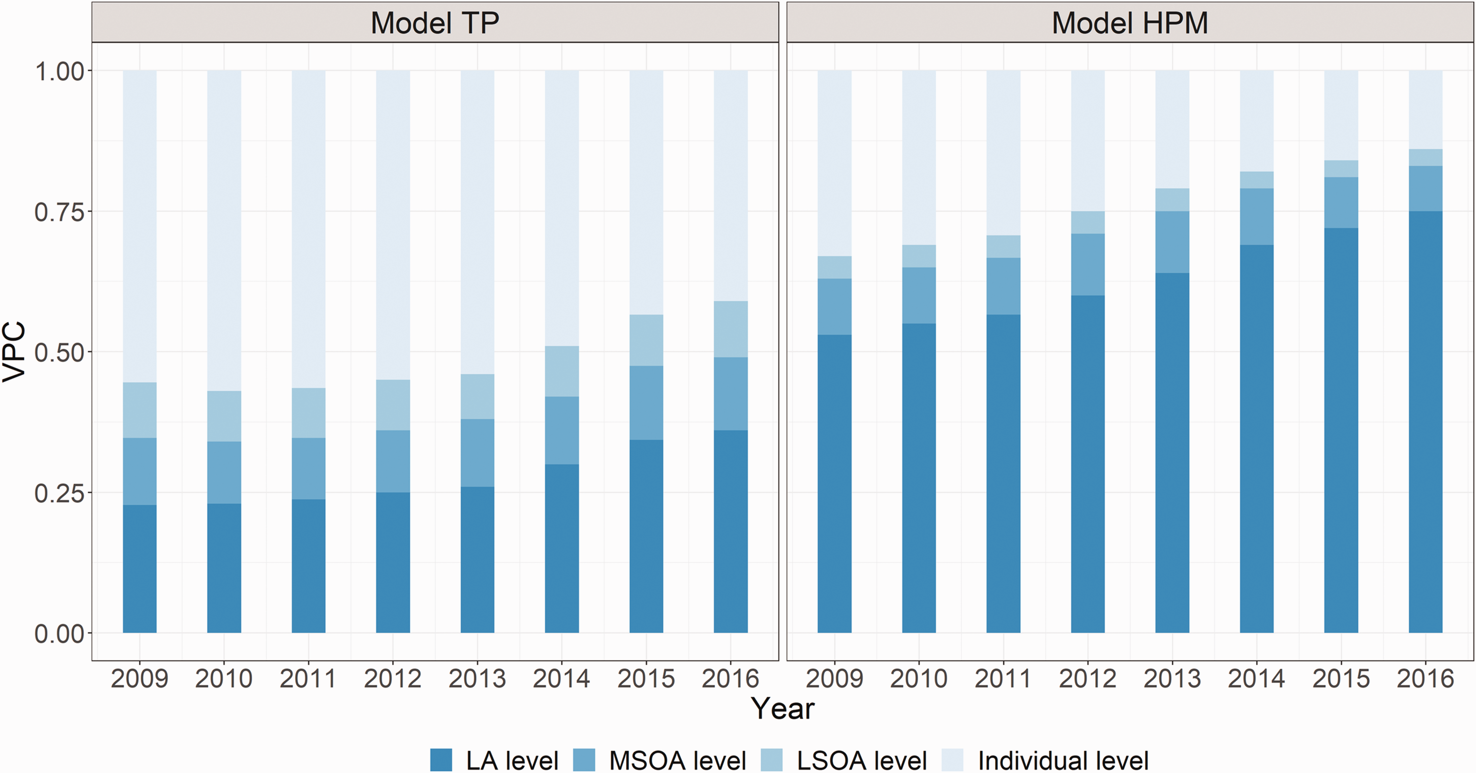
VPC results for model TP and HPM. HPM: house price per square metre; LA: local authority; LSOA: Lower Layer Super Output Area; MSOA: Middle Layer Super Output Area; TP: transaction price; VPC: variance partition coefficients.
HPM clustering at four geographic levels between 2009 and 2016
The ICC at a given level shows the degree of house price clustering. The ICC results of model HPM are presented in Table 2. ICC at LA level is 0.53 in 2009 and continues increasing to 0.75 by 2016, illustrating that HPM are clustered at LA level. ICC at MSOA level is 0.63 in 2009 and continues increasing to 0.83 by 2016. Meanwhile, the ICC at MSOA level shows negligible improvement at LSOA level. This suggests that HPM at MSOA level are highly clustered and variations within the same MSOA unit are quite small between 2009 and 2016. This also suggests that using the mean HPM at MSOA level gives a relatively clear house price picture (2009–2016) and very little additional explanatory power is gained from observing house price variations at a more granular geographical scale. This may reflect the similar population based criteria (Study area and geographical scales section) used in creating LSOA and MSOA boundaries giving rise to similar density patterns.
ICC results for the HPM models.
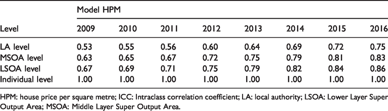
HPM: house price per square metre; ICC: Intraclass correlation coefficient; LA: local authority; LSOA: Lower Layer Super Output Area; MSOA: Middle Layer Super Output Area.
HPM variation at LA level
The ICC at MSOA level is equal to the VPC at MSOA level plus LA level. Owing to a noticeable VPC increase at LA level between 2009 and 2016, ICC at MSOA level shows a strong increase. HPM became more highly clustered at MSOA level between 2009 and 2016 as shown by the increase in ICC, which is largely due to the noticeable VPC increase at LA level. Owing to the total HPM variance increases between 2009 and 2016 (Figure C1.B), increasing house price variance at LA level is the main reason behind the VPC increase between 2009 and 2016 (Figure 2). Figure 3 is a graphical illustration of this increasing variation from 2009 to 2016 and shows estimated residuals at LA level (
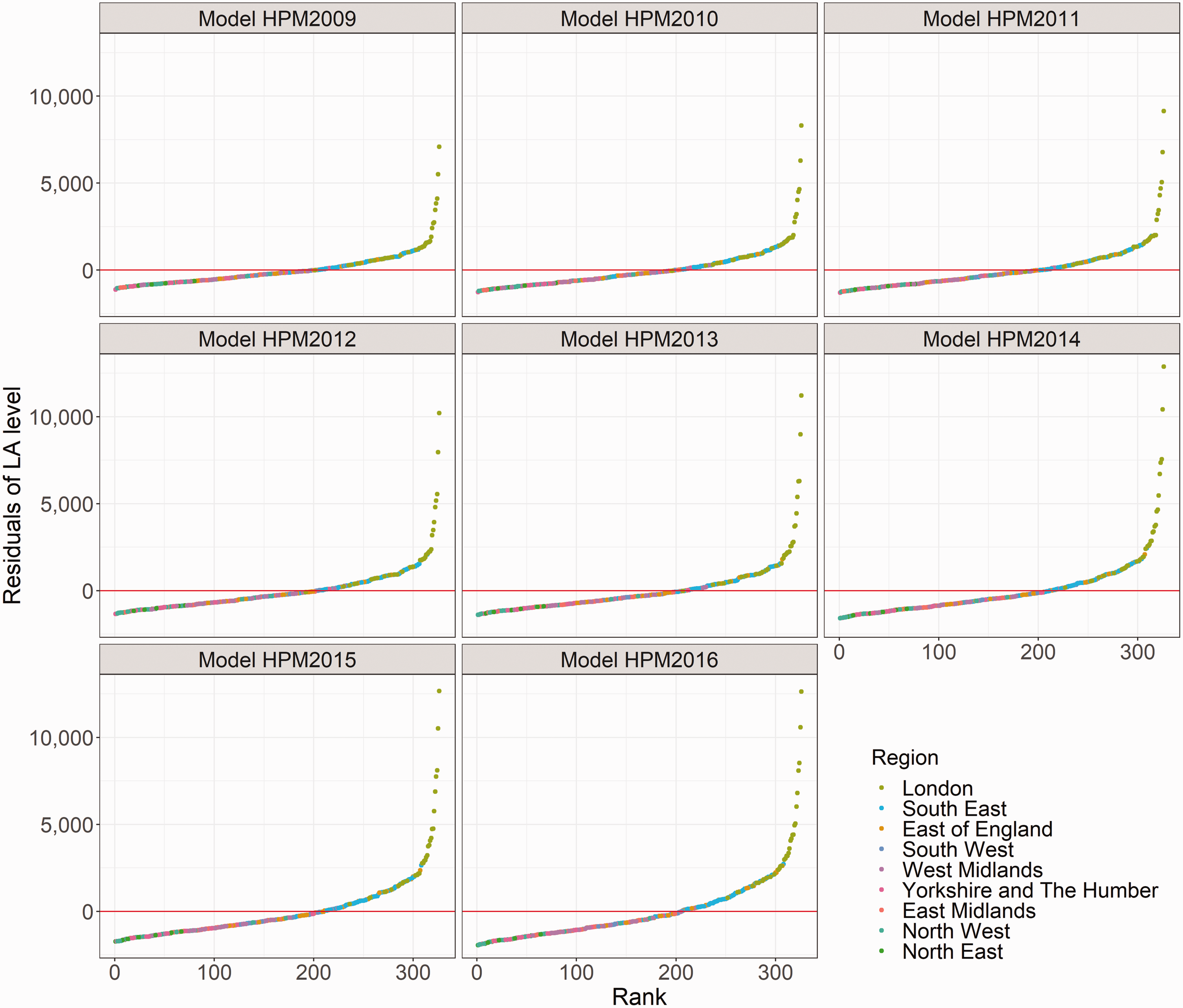
Residuals at LA level in England in the HPM models. HPM: house price per square metre; LA: local authority.
Examining LA residuals further by plotting them for different regions (supplementary material D), shows that, with the exception of Barking and Dagenham, LAs’ house prices in London are consistently above the overall mean house price in England, with a continuously widening house price difference. London can be classed as an ‘outlier’ region in England and maintains its position as the most expensive region. London’s LAs display a more rapidly increasing house price than the LAs in other regions. This London effect dominates the increasing house price variation at LA level from 2009 to 2016. Meanwhile, relatively small house price increases in the North East and the East of England also make a small contribution to the widening differential in regional house prices.
London’s LA HPM variation
Figure 4 displays LA residuals in London (third column plots in supplementary material D) and offers a graphical illustration of London’s increasing HPM variation from 2009 to 2016. Most LAs in London have a mean price lower than £2000 per square metre. Kensington and Chelsea consistently comes top in this ranking, followed by Westminster and then Camden. Some other LAs also show a substantial increase in house prices, contributing to the increasing LA house price difference. For example, Southwark, Lambeth, Hackney and Tower Hamlets were lower than £2000 per square metre level (grey dashed line) from 2009 to 2011, but after that, their increasing prices started to exceed the £2000 per square metre level. Consequently, HPM at LA level in London have become more polarised, with central and south-western boroughs such as Westminster, Kensington and Chelsea, Hammersmith and Fulham, Camden and Richmond pulling further away from the £2000 per square metre level.
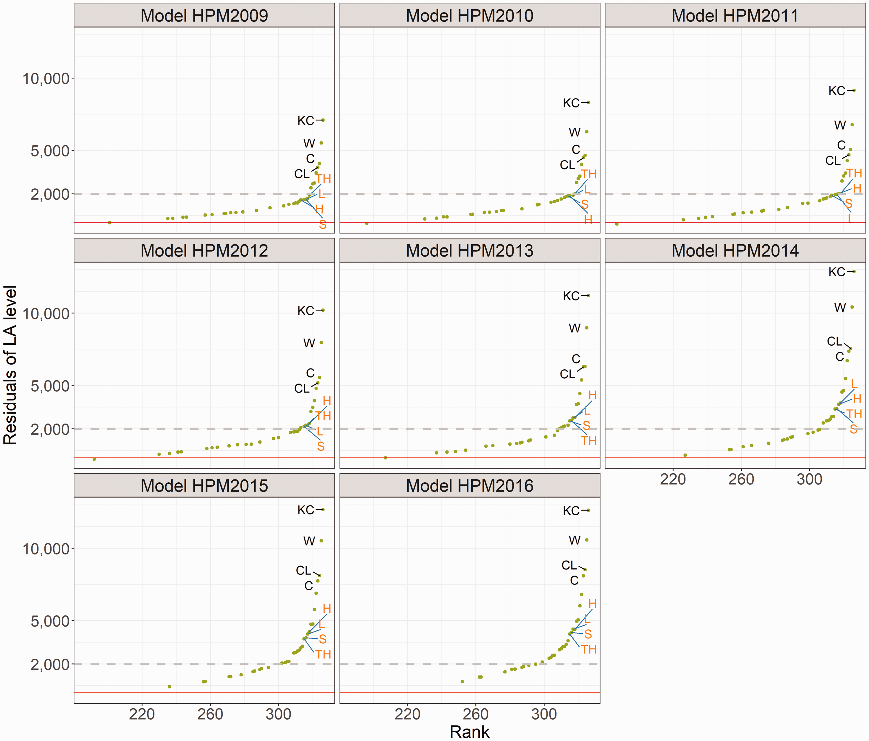
Residuals at LA level in London in the HPM models. C: Camden; CL: City of London; HPM: house price per square metre; KC: Kensington and Chelsea; H: Hackney; L: Lambeth; LA: local authority; S: Southwark; TH: Tower Hamlets; W: Westminster.
Looking at the rank of LA residuals within London (Supplementary materials E), Kensington and Chelsea consistently tops the price league with five other central London boroughs (Westminster, Camden, City of London, Hammersmith and Fulham, and Islington) consistently high (yellow text in supplementary materials E and F). At the other end of the scale, Barking and Dagenham consistently exhibits the lowest prices. Ten LAs that increased their rank order from 2009 to 2016 are mainly located in outer London to the east and southwest of the centre (Green text label in supplementary materials E and F).
London’s HPM effect in England’s housing market
London’s high HPM also affects neighbouring housing markets. Supplementary material G displays the residuals at LA level in England at 2009 with a separate map of housing markets near London. Residuals at LA level in England are grouped into eight sub-groups using the natural breaks method. The LAs with darker shades show relatively high house prices when compared to the price in England. These relatively high price areas in the ‘Home Counties’ in the South East and the East of England are all within the commuter belt, with many living in these areas still working in London and properties consequently being linked to the London housing market. The 11 LAs labelled in supplementary material G are all in the top 30 price league in England in 2009 in terms of HPM. London’s effect on the South East appears to be stronger than on the East of England, which could well correspond to the higher density of commuter rail routes to the South West of the capital when compared to the North East.
Setting aside London’s effect within its housing market and on the housing market in nearby LAs, the HPM still shows considerable variability at LA level in the remaining eight regions. There are three groups of LAs exhibiting relatively high price areas distant from London. These are on the South coast – South Ham, Christchurch and East Dorset; the Cotswolds, straddling the north east part of the South West, the West and East Midlands; and moving to the North of England, a third group comprising contiguous LAs near to large national parks (e.g. South Lakeland). LAs within these three groups also contribute to house price differentials at LA level. Interestingly, the London effect may still be operating here, as these areas are characterised by relatively high volumes of second-home ownership, with owners registering other homes in London (Dennett, 2013).
Conclusions and future research
Understanding the nature and extent of differentials in property prices at different geographical levels leads to a better understanding of housing markets. This study compares house price variation in TP and HPM across England by using a new linked dataset. Examining HPM in this way exposes spatial differences (obscured by differences in local stock mix and transaction patterns) more prominently. This confirms that HPM offers a more meaningful picture of house price variation than TP alone. Examining house price variation at four geographic scales across England using a four-level variance components model suggests that house price drivers operate differently at different geographical scales and that these effects changed between 2009 and 2016. House price differentials between LAs are quite large and this spatial effect increases at MSOA level. HPMs are generally very similar within MSOAs, with little to be gained from exploring variations at the lower LSOA level. This is a useful practical finding and demonstrates that aggregating HPM at MSOA level might be sufficient to give a clear picture of local housing markets or sub-markets in England.
Overall house price variability in England shows an increase from 2009 to 2016. In 2009, 53% of house price variation existed between LAs. The magnitude of disparities increased 1.42 times in the following eight years. This increasing imbalance follows from London’s house prices increasing more rapidly than that of any other region. While looking at HPM variation between LAs by plotting the residuals of LA level change, we found that some LAs in the central part of London are the main source of this increasing LA effect. Moreover, London affects not only house price differences between regions but also its nearby LAs. LAs in the South East and East of England which are near to London show the highest house price within their regions. Of the top 30 LAs with the most expensive house prices, 19 of them are located in London and the remaining 11 LAs are located outside London but within its travel-to-work area. The current housing policy (e.g. Right to Buy) which differentiates between London and the rest of the UK would be more consistent if based on HPM, thus including some of the more expensive areas bordering London. Excepting the LA housing markets nearby London, some LAs near South Ham, Cotswold and South Lakeland also show high house price spatial clustering. These areas contribute to house price imbalances after excluding the near-London effect.
This research has demonstrated that multilevel variance components modelling can offer a model-based descriptive analysis for the exploration of house price variation at multiple geographic scales, providing a new insight into spatial house price disparities across England. Having created a new time-series dataset linking TPs to a variety of housing attributes and having established a methodology, we intend to extend this work through a more thorough exploration of house price variance at LA and MSOA level by considering the interacting effects of time, location and key local factors such as plot size, land use structure, housing density, local physical and socio-economic environments. Understanding the underlying mechanisms of house price variation offers the potential for deeper insights into pressing housing inequality issues in England.
Supplemental Material
sj-pdf-1-epb-10.1177_2399808320951212 - Supplemental material for Shedding new light on residential property price variation in England: A multi-scale exploration
Supplemental material, sj-pdf-1-epb-10.1177_2399808320951212 for Shedding new light on residential property price variation in England: A multi-scale exploration by Bin Chi, Adam Dennett, Thomas Oléron-Evans and Robin Morphet in Environment and Planning B: Urban Analytics and City Science
Footnotes
Acknowledgements
The authors would like to thank Mrs Jane Galbraith and Professor Kelvyn Jones for providing valuable guidance and basic knowledge of variance analysis. The authors also would like to thank Rob Liddiard for sharing his expertise regarding EPC data during the earlier stages of this research.
Declaration of conflicting interests
The author(s) declared no potential conflicts of interest with respect to the research, authorship, and/or publication of this article.
Funding
The author(s) disclosed receipt of the following financial support for the research, authorship, and/or publication of this article: This research was funded by the China Scholarship Council (CSC No. 201708060184).
Supplemental material
Supplemental material for this article is available online.
Note
References
Supplementary Material
Please find the following supplemental material available below.
For Open Access articles published under a Creative Commons License, all supplemental material carries the same license as the article it is associated with.
For non-Open Access articles published, all supplemental material carries a non-exclusive license, and permission requests for re-use of supplemental material or any part of supplemental material shall be sent directly to the copyright owner as specified in the copyright notice associated with the article.