Sage Journals: Discover world-class research

Abstract

Urban settlements and urbanised populations continue to grow rapidly and much of this transition is occurring in less developed countries. Remote sensing techniques are now often applied to monitor urbanisation and changes in settlement patterns. In particular, increasing availability of very high resolution imagery (<1 m spatial resolution) and computing power is enabling complete sets of settlement data in the form of building footprints to be extracted from imagery. These settlement data provide information on the changes occurring in cities, particularly in countries which may lack other data on urbanisation. While spatially detailed, extracted building footprints typically lack other information that identify building types or can be used to differentiate intra-urban land uses or neighbourhood types. This work demonstrates an approach to classifying settlement types through multi-scale spatial patterns of urban morphology visible in building footprint data extracted from very high resolution imagery. The work uses a Gaussian mixture modelling approach to select and hierarchically merge components into clusters. The results are maps classifying settlement types on a high spatial resolution (100 m) grid. The approach is applied in Kaduna, Nigeria; Kinshasa, Democratic Republic of the Congo; and Maputo, Mozambique and demonstrates the potential of computational methods to take advantage of large spatial datasets and extract meaningful information to support monitoring of urban areas. The model-based approach produces a hierarchy of potential clustering solutions, and we suggest that this can be used in partnership with local knowledge of the context when creating settlement typologies.

Keywords

Urban morphology land use classification spatial analysis urban analytics

Introduction

Urban settlements and urbanised populations have been growing at unprecedented rates around the world (Seto et al., 2010; UN Department of Economic and Social Affairs, 2019). By 2050, the United Nations predicts 68% of the world’s population will live in cities and towns, and most of this change will be occurring in low- and middle-income countries (UN Habitat, 2016). This transition towards more urbanised living has potential to impact health, livelihoods, and family structures (Benza et al., 2017; WHO & UN-Habitat, 2010). Urban sprawl and megacities are a dramatic and visible change on the landscape and a major cause of vegetation loss (McDonald et al., 2008), and the growth of slums and informal settlements within cities is a concern for potential adverse health exposures and environmental risks (UN Habitat, 2016; WHO & UN-Habitat, 2010). Yet at the same time, well-designed and managed urban areas have the potential to improve sustainability and more efficiently provide services, access to facilities, and resources to larger numbers of people (Seto et al., 2010). These tensions in the transition towards urbanising populations have gained attention from policy makers. The Sustainable Development Goals and the UN New Urban Agenda specifically seek to leave no one behind while creating inclusive, safe, environmentally sustainable, and healthy cities (UN General Assembly, 2017). These development goals highlight that urban areas are not homogenous in their development needs, and they require more detailed, disaggregated data to monitor these issues. In recent years, remotely sensed earth observation data and imagery, with consistent mapping over large areas, has frequently been used to monitor city growth and urbanisation patterns (Irwin and Bockstael, 2007; Luck and Wu, 2002; Schneider and Woodcock, 2008; Taubenböck et al., 2012). Improvements in sensor technology, combined with growing computational power, are enabling a new trend towards mapping larger areas of the globe at ever finer resolutions (Patlolla et al., 2012; Roy Chowdhury et al., 2018). Very high resolution (VHR) imagery, with pixel resolutions of less than 1 m, makes even small objects detectable in visible and near infrared imagery. VHR imagery has been used to monitor changes and to classify land uses within urban areas (Graesser et al., 2012; Kuffer et al., 2014), but such imagery requires different analysis approaches using object-based classification and textural features instead of methods based on per-pixel spectral indices (Engstrom et al., 2015; Kit et al., 2012; Kuffer et al., 2016). Advances in image processing are using the pixel-based textures in the imagery to segment meaningful objects (Cheriyadat et al., 2007; Yuan et al., 2015) as well as machine learning algorithms to produce detailed maps of urbanisation by detecting and extracting all built features visible in imagery scenes (Yuan, 2016). For example, Microsoft has used neural networks to produce complete building footprint datasets from imagery for the US and Canada (Bing Maps Team, 2018, 2019). These automated extraction approaches are building on efforts such as OpenStreetMap (http://www.osm.org) and crowd-sourced efforts to manually digitise structures from imagery. These efforts, and others, have produced a range of outputs mapping human settlements at different spatial resolutions (Roy Chowdhury et al., 2018).

Imagery-derived building datasets can provide valuable information for monitoring cities and the extents of urban areas, particularly in places without detailed planning maps or cadastral data. However, building footprints generally lack information about the building types or land uses and are only binary maps of settled versus unsettled areas. Despite the limited attribute information, patterns in the building features can suggest local land uses (Barr et al., 2004; Steiniger et al., 2008). Individual buildings form the basis of the built landscape and the broader patterns of building density, size, shapes, and orientations can convey information about land use and economic activities (Steiniger et al., 2008). Our perceptions of these morphological and spatial patterns follow from Gestalt principles (Li et al., 2004; Steiniger et al., 2008). These psychological principles describe how we organise and group visual elements based on their proximity and similarity in size or orientation. These types of visual patterns in spatial data of buildings have been used to classify regular and irregular neighbourhood types (Yan et al., 2019) or more nuanced functional areas (Steiniger et al., 2008), to classify individual buildings (Hecht et al., 2015), predict buildings’ ages (Rosser et al., 2019), and as part of automated cartographic generalisations (Lüscher and Weibel, 2013).

The present work addresses the challenge of classifying settlement types at a high spatial resolution to characterise intra-urban differences. Such maps can support urban planning and studies of urbanisation patterns (Seto et al., 2010) and population distribution (Grippa et al., 2019). Identifying areas of distinct settlement patterns, such as from building footprint data, can help to guide survey data collections and statistical models used to make population estimates (Wardrop et al., 2018). We utilise one of the new sources of building footprints extracted from VHR imagery produced by Ecopia (http://www.ecopiatech.com). As noted above, these datasets lack detailed attribute information, and the goal of our work is to extract new information from the spatial patterns of these built-up features alone. We draw on previous work (Benza et al., 2016; Seto and Fragkias, 2005) of using fragmentation statistics (McGarigal et al., 2008) to quantify the patchiness, connectivity, and shape of the urban form. We use a model-based clustering procedure (Fraley and Raftery, 2003) to identify and map settlement types, and we implement our full approach in a high-performance computing environment.

Materials

Study areas

The sites of Kaduna, Nigeria; Kinshasa, Democratic Republic of the Congo; and Maputo, Mozambique were selected to test the classification approach. These regions were chosen for the availability of recent building footprint datasets as well as to explore a variety of less developed country contexts. Each site includes a mix of land uses within a large urban center in addition to outlying settlements, and more sparsely settled rural areas. The extent of the study sites are shown in Figure 1, and we refer to them throughout the paper by their main urban center: Kaduna, Kinshasa, and Maputo, respectively.

Figure 1.

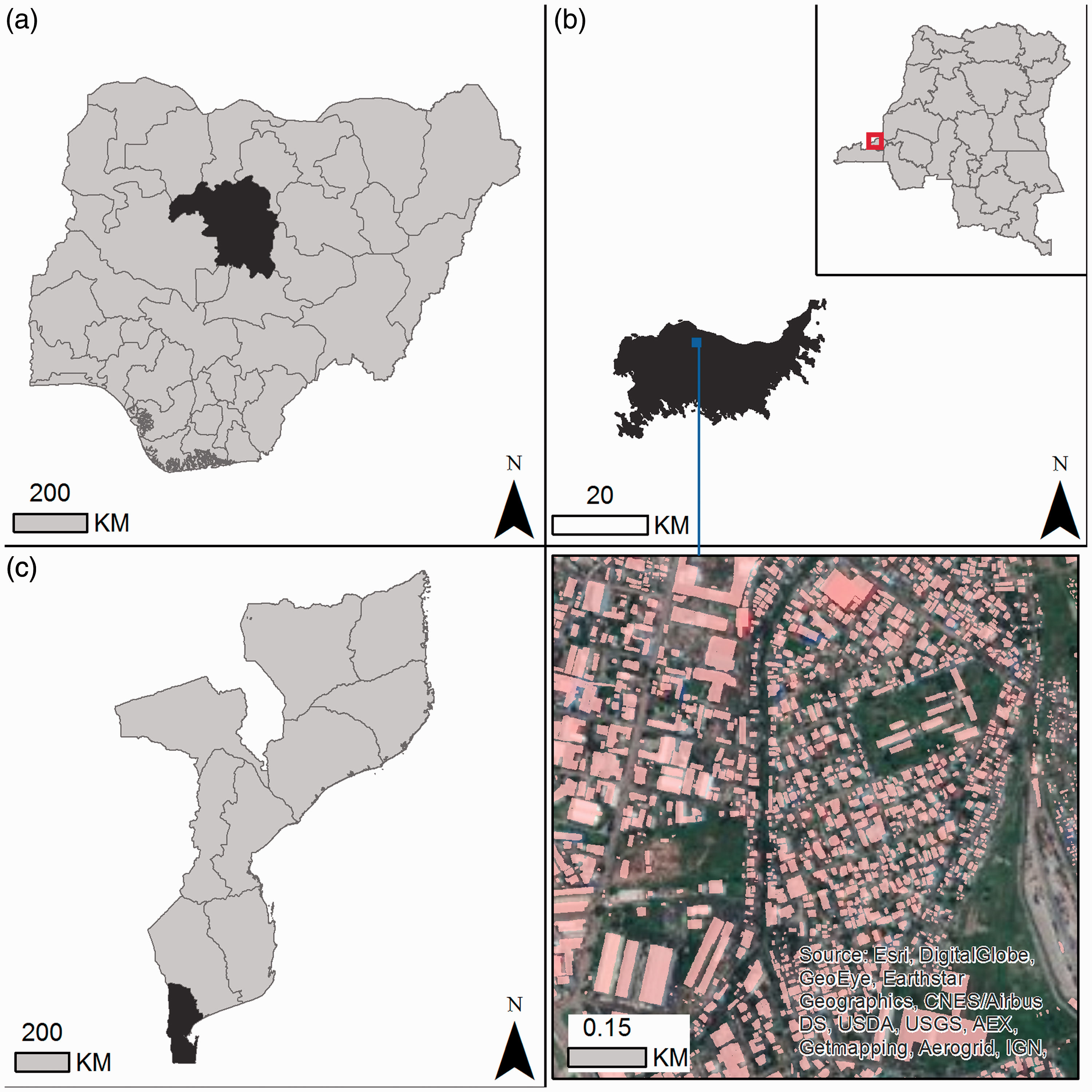
Study areas of Kaduna, Nigeria (a), Kinshasa, Democratic Republic of the Congo (b), and Maputo, Mozambique (c). The extent of the building footprint datasets are shown in dark grey. An example of the building features from an area of Kinshasa is shown in the lower right quadrant. (Data source: © 2020 Maxar Technologies, Ecopia.AI.).

Building footprint data

We use a new dataset (© 2020 Maxar Technologies, Ecopia.AI) of building footprints produced by Ecopia in partnership with Maxar (formerly DigitalGlobe). These feature data are extracted from imagery mosaics with 50 cm spatial resolution or better, using artificial intelligence methods (DigitalGlobe, 2018). Accuracy and completeness statistics were not available in our specific study areas, but all extracted features pass several automated checks for valid geometries and for every 1000 km² of processed area, 50 km² is randomly selected and features are manually digitised and compared to reach 95% completeness (Ecopia and DigitalGlobe, 2017). The output of the Ecopia processing is a set of polygon features representing building footprints. There were 2,298,272 features in Kaduna, 1,118,386 in Kinshasa, and 1,258,369 in Maputo. These building features are unlabelled – they contain no attribute information about the structures such as height or use. An example of the building features is shown in Figure 1. We note that the extraction process does not always produce polygons with straight edges or square corners. This initial observation prompted us to explore a landscape perspective of settlement patterns with raster-based analyses rather than methods that rely on building-specific measurements (Barr et al., 2004) and require geometrically accurate shapes. Prior to processing, we converted the polygons to binary rasters with a 1 m spatial resolution in their local WGS 84 UTM coordinate system. The choice of resolution was to reduce file size. One consquence of the conversion is that features which are smaller than 1 m × 1 m are excluded, though these are unlikely to be meaningful structures.

Methods

In our approach, the mapped footprints are treated as patches in the landscape and a variety of metrics are used to quantify their morphological patterns. These types of calculations have their origins in landscape ecology (McGarigal, 2015; McGarigal et al., 2008) but have been used previously to quantify morphological patterns of cities using built-up areas from land cover maps (Benza et al., 2016; Luck and Wu, 2002; Seto and Fragkias, 2005). We extend such work to classify high-resolution areas within the study region based on the combination of patterns at multiple spatial scales. We do this by defining a set of processing locations covering the study areas on a regular grid at 3 arc-second spatial resolution (approximately 100 m × 100 m). This resolution was chosen to match other geospatial datasets (Lloyd et al., 2019) as our intention in future work is to compare settlement classifications with other demographic datasets. At each location, we calculated seven different metrics of the building patterns within a circular neighbourhood. The radius of the circular neighbourhood was varied in 50 m increments from 50 m up to 500 m in order to quantify spatial patterns at multiple spatial scales. Therefore, for each location in the 100 m grid, there were 70 values (7 metrics × 10 spatial scales). The processing steps are further explained in the supplemental materials (Section 1). The metrics are described in detail in the next section.

Spatial metrics

Previous studies of urban morphology and building features have shown the importance of quantifying density, size, and shape (Benza et al., 2016; Jochem et al., 2018; Roy Chowdhury et al., 2018). Examples of the building patterns associated with each metric are shown in Section 3 of the supplemental materials. We quantified the density of buildings as the number of patches per area

Patch Density = \frac{n}{A}

(1)where n is the count of patches and A is the total area of the processing window. Within a fixed area, increasing patch density implies more structures, which may be smaller or more tightly spaced. Two metrics are used to explore the size of building footprints. The first is the average area of all patches within the processing window

Mean Patch Area = \frac{1}{n} \sum_{i = 1}^{n} a_{i}

(2)where a_i is the area of the i-th patch within the processing window. The variability in the size of patches is summarised by the coefficient of variation (CV)

Patch Size C V = \frac{\sqrt{\frac{\sum_{i = 1}^{n} {(a_{i} - (\sum_{i = 1}^{n} a_{i}))}^{2}}{n}}}{\frac{\sum_{i = 1}^{n} a_{i}}{n}}

(3)

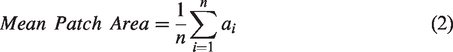
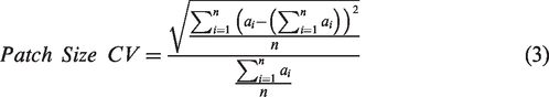
The CV expresses variation in building footprint sizes as the ratio of standard deviation in patch sizes to the average patch size within the processing window. Areas with a high CV might suggest a less planned area, mixed building uses, or a transition area between two settlement types – from larger administrative/commercial structures to small housing, for example.

The shape and regularity of patches are summarised with a landscape shape index and an average patch shape index. Both metrics are based on standardised measures of the perimeters, and higher values are found in areas with more irregularly shaped structures, which could be associated with less planned urbanisation.

Landscape Shape Index = \frac{0.25 E}{\sqrt{A}}

(4)where 0.25 is an adjustment for using raster data and E is the total edge length of patches in the area of the processing window, A. The average patch shape index is defined by each patch’s edge length, e, relative to a minimum size possible given its area (

\min (e)

)

Shape Index = \frac{e}{\min (e)}

(5)

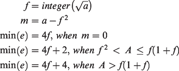
The value for $\min (e)$ depends on the minimum perimeter for a compact square shape of area a. This can take one of three forms (Bogaert et al., 2000).

\begin{array}{l} f = integer (\sqrt{a}) \\ m = a - f 2 \\ \min (e) = 4 f, when m = 0 \\ \min (e) = 4 f + 2, when f 2 < A \leq f (1 + f) \\ \min (e) = 4 f + 4, when A > f (1 + f) \end{array}

The shape index can be interpreted as a degree of aggregation of the patch, while a fractal dimension is used to quantify the complexity in those patch shapes.

Fractal Dimension Index = \frac{2 \ln (0.25 p)}{\ln (a)}

(6)where p is the perimeter of each patch with area, a. We used the average of the index values for patches within the processing window. Structures with simple shapes have low values, and a low average fractal index within the processing window could suggest more regular or planned settlements.

Finally, we use a patch cohesion index to measure the level of connectedness of the patches in each window. Areas with low cohesion are characterised by small, separated structures, while high cohesion is seen among central areas with a fewer, large, agglomerated structures.

Patch Cohesion Index = (1 - \frac{\sum_{i = 1}^{n} p_{i}}{\sum_{i = 1}^{n} p_{i} \sqrt{a_{i}}}) \cdot {(1 - \frac{1}{\sqrt{Z}})}^{- 1} \cdot 100

(7)where p is the perimeter of each patch, i, with area, a, and Z is the total number of cells within the processing widow.

The landscape metrics, calculated across spatial scales, show strong correlation. Additionally, the metrics are on different response scales and have different ranges of possible values but need to be combined in the clustering algorithm. Therefore, to reduce the correlation and to highlight the patterns of variation, the standardised data (mean centred and scaled by the standard deviation) are used for principal components analysis. We select the minimum set of components that explained 90% of the variation in each metric across scales. Principal components were calculated in R with prcomp (R Core Team, 2017).

Classification

After calculating the range of metrics, the next phase of processing is to classify patterns. This step identifies the important differences in combinations of metrics (see example in supplemental material, Section 3). We applied a multi-step model-based clustering procedure (Fraley and Raftery, 2003; McNicholas, 2016). Specifically, we used a Gaussian finite mixture model implemented in MCLUST version 5 software and the functions of the R package mclust (Scrucca et al., 2016). This implementation allows for different combinations of equal or varying quantities in the covariance to describe the volume, shape, and orientiation of the ellipsoidal clusters in multivariate data space. This flexibility helps to find more irregular or overlapping clusters in the data. Following Fraley and Raftery (2003), we use similar notations to describe these model forms as equal (“E”) or varying (“V”) such that a “VEV” model has equal shapes with varying volumes and orientations of components while “VVV” is fully varying. Selecting the number of components and parameterisation for the best fitting model is guided by a Bayesian Information Criterion (BIC) calculation (Scrucca et al., 2016).

Mixture models can be computationally burdensome for large datasets. We used a data sampling and model comparison approach suggested by Wehrens et al. (2004). We tested a range of different covariance structures in the MCLUST software and the top six candidate models were selected to achieve the best BIC (Table S2 and Figure S2). The top models were then re-fit using the full set of pixels, and the final model form and number of compenents was selected to maximise the log-likelihood. More details are given in Section 4 of the supplemental material.

Many applications of mixture models for model-based clustering treat the selected number of mixture components to be the number of clusters. However, model selection guided by BIC often suggests a larger number of components to fit the data than there are well-separated clusters in the data (Baudry et al., 2010; Hennig, 2010). This difference can occur when there are overlapping clusters or when clusters are not Gaussian. Multiple solutions to identify clusters from a larger set of components have been suggested (Hennig, 2010), including likelihood ratio tests (McLachlan and Rathnayake, 2014), alternative information criteria such as the integrated complete-data likelihood (Biernacki et al., 2000), or connected components (Scrucca, 2016). We used a process to hierarchically merge the components of the top model in order to minimise a measure of entropy (Baudry et al., 2010). The result was a stepped grouping of components into a range of clusters, from two up to a maximum when each component is treated as a cluster. In order to select the final number of clusters for each study area, we examined plots of the change in entropy with each merging step as well as the output prediction maps to select a parsimonious grouping that still maintained intra-urban variation in settlement patterns. Baudry et al. (2010) recommend choosing a grouping of components that produces meaningful cluster types while guided by aims of reducing entropy.

After selecting the number of clusters, we made a final map of predicted settlement type. Each pixel was classified based on a maximum predicted probability of cluster membership. We applied a 3 × 3 majority filter to minmially smooth the predicted classes. Each study area was processed separately so component numberings may vary. To facilitate comparison among areas, we relabeled the clusters numerically in order of descending average patch density at 100 m scale. We chose a numeric class labelling instead of attempting to provide class names (i.e., “residential”, “industrial”, etc.) to take a more exploratory approach of the unsupervised classification results and to avoid subjectivity in the labelling.

Results

For each of the three study areas, sets of 70 data layers were produced from the landscape feature calculations (7 features × 10 spatial scales). Custom Python scripts were written to implement the feature calculations and the moving window operations in parallel. The data layers were centred, scaled, and reduced to 18 principal component layers each for Kaduna and Kinshasa and 19 layers for Maputo. Details on the components selected are provided in the supplemental materials (Table S1). The loadings for the principal components are shown in the supplemental materials (Figure S1).

The reduced sets of layers were used for the model-based clustering, and BIC values were used to compare models. Across the three areas, the fully varying model (“VVV”) was always chosen with between 6 and 13 components. The candidate models are summarised in the supplemental materials (Table S2). The full set of BIC values are shown in the supplemental materials (Figure S2). The best performing model for each study area was selected by maximising the log-likelihood. In all three study areas, the largest number of components among the top candidate models (11 for Kaduna, 12 for Kinshasa, and 13 for Maputo) was selected as the best performing model.

Starting from the maximum number of components suggested in the model selection step, the goal was to reduce these components to a smaller number of interpretable clusters based on an entropy criterion (Baudry et al., 2010), which provided a sequence of hierarchical merging solutions to minimise this criterion. The results of the entropy calculations are shown in Figure 2 as both a plot of entropy versus the number of clusters as well as a dendrogram plot of the suggested components to merge at each step. Lower branches on the dendrogram correspond to more clusters, but also higher entropy. Also included in each plot of entropy versus number of clusters is a two-segment piecewise linear model which Baudry et al. (2010) suggest could indicate an optimal number of clusters. The plots all show almost linearly increasing entropy scores without a clear “elbow”. The minimal break points of the piecewise model suggested combining components into smaller numbers of clusters: four clusters for Kaduna and Maputo, and five clusters for Kinshasa.

Figure 2.

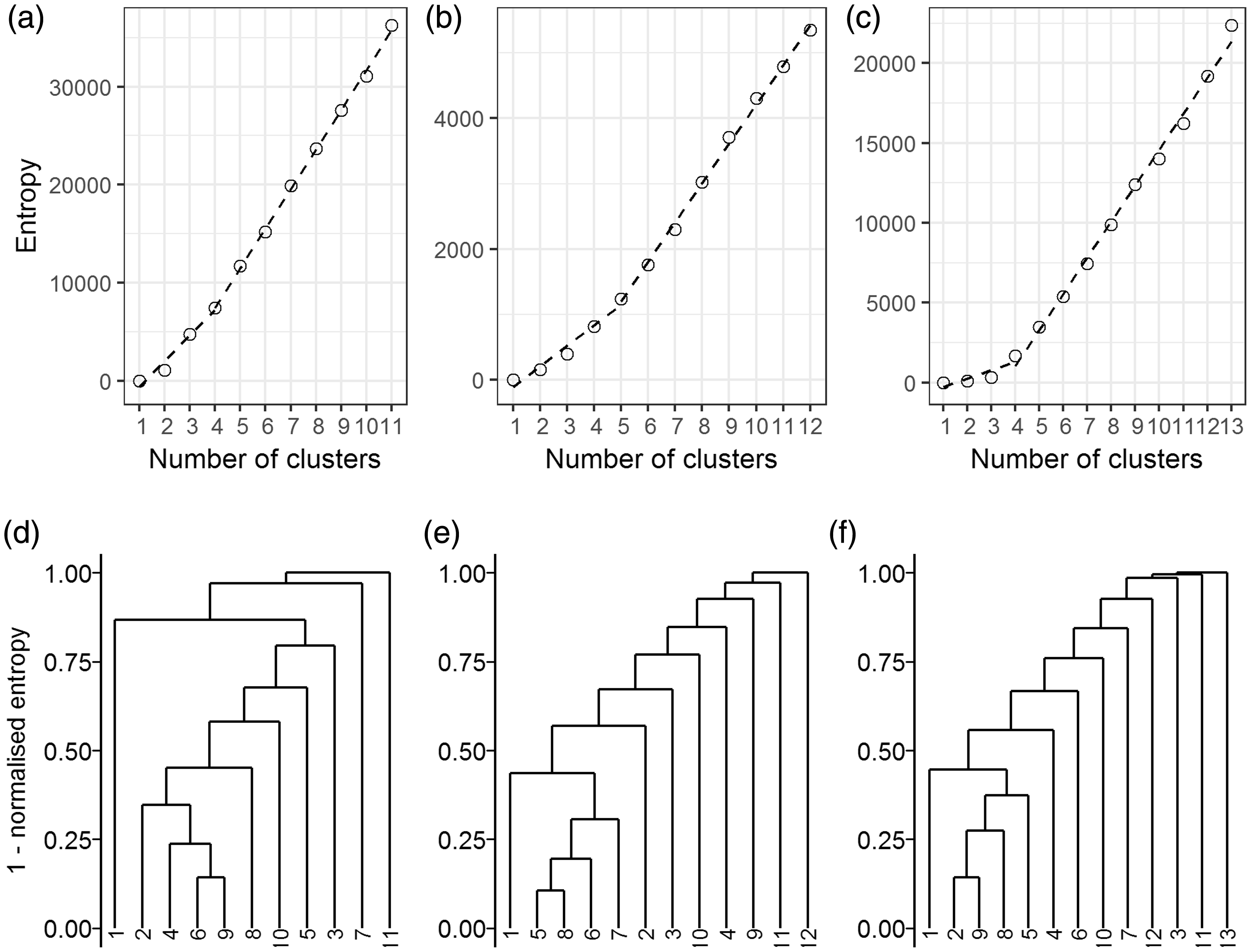
Results of merging mixture model components to reduce entropy scores in potential clusters. Plots of the entropy versus the number of potential clusters (top row) include a piecewise linear model with a breakpoint suggesting the minimum number of clusters for Kaduna, Nigeria (a), Kinshasa, Democratic Republic of the Congo (b), and Maputo, Mozambique (c). The merging of components creates a hierarchy of potential clusters and settlement types as shown in the bottom row dendrogram plots for Kaduna (d), Kinshasa (e), and Maputo (f).

In the dendrogram calculated for Kaduna, there were three clearly distinct clusters forming from the components, while a fourth cluster is potentially made from multiple components. Kinshasa and Maputo show similar patterns but to a lesser extent. In each site, four components appear to form a grouping, though the remaining components were not clearly separated.

Examples of the predicted settlement type maps at 100 m spatial resolution for Kinshasa are shown in Figure 3 using the 12 cluster solution and with the reduced 5 cluster solution in Figure 4. Predictions for Kaduna and Maputo study areas are shown in the supplemental materials (Figures S3 to S6). While the model-based clustering method does not consider spatial configurations of the data, geographic groupings of settlement types clearly emerge. In Kinshasa, large structures, such as for warehouses or industrial use, remain one of the distinct types and are found predominantly in the northern part of the city. Rural areas are also predicted into distinct settlement types made up of small, patchy building footprints along the southern and eastern edges of the study area. The large number of different classes along the southern edge of the main urban area are combined into one settlement type after the merging step (creating type 2 in Figure 4). The five settlement type solution continues to show differences in settlement types within the core area of Kinshasa (shown in Figure 4).

Figure 3.

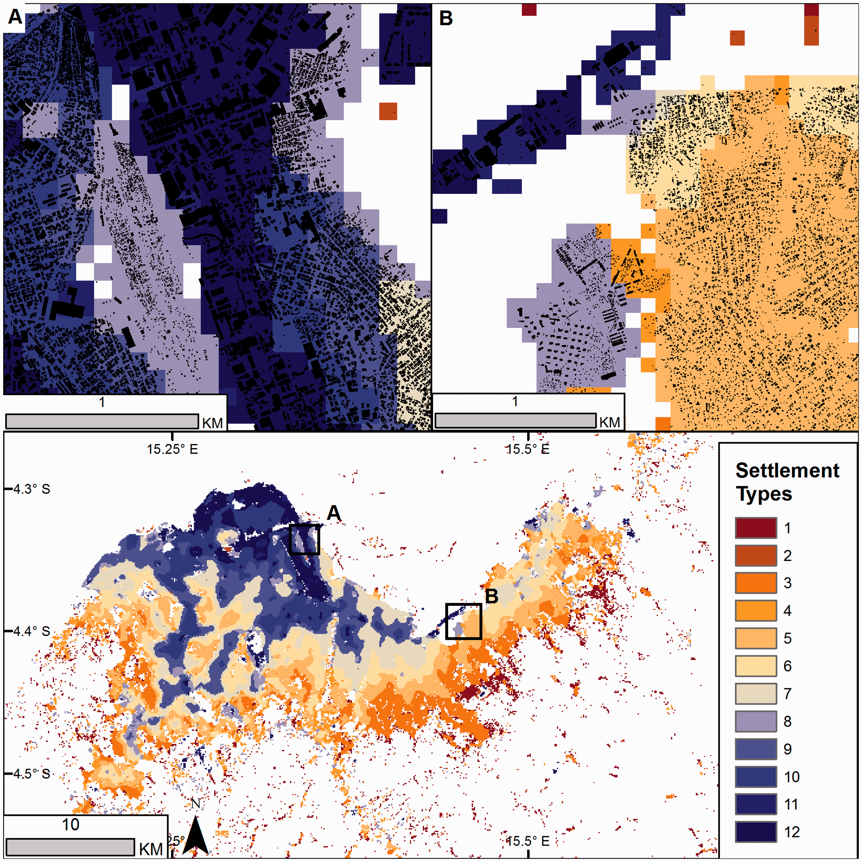
Predicted settlement types for Kinshasa, Democratic Republic of the Congo, at 100 m spatial resolution. Clusters are defined by Gaussian mixture model components using spatial patterns of building footprints. Examples of the building footprints are shown in the inset maps (a) and (b), overlaid on the predicted types. A 3 × 3 majority smoothing filter was applied to the predicted classes. Clusters are labelled in decreasing average patch density. Whitespace in the maps are unsettled pixels.

Figure 4.

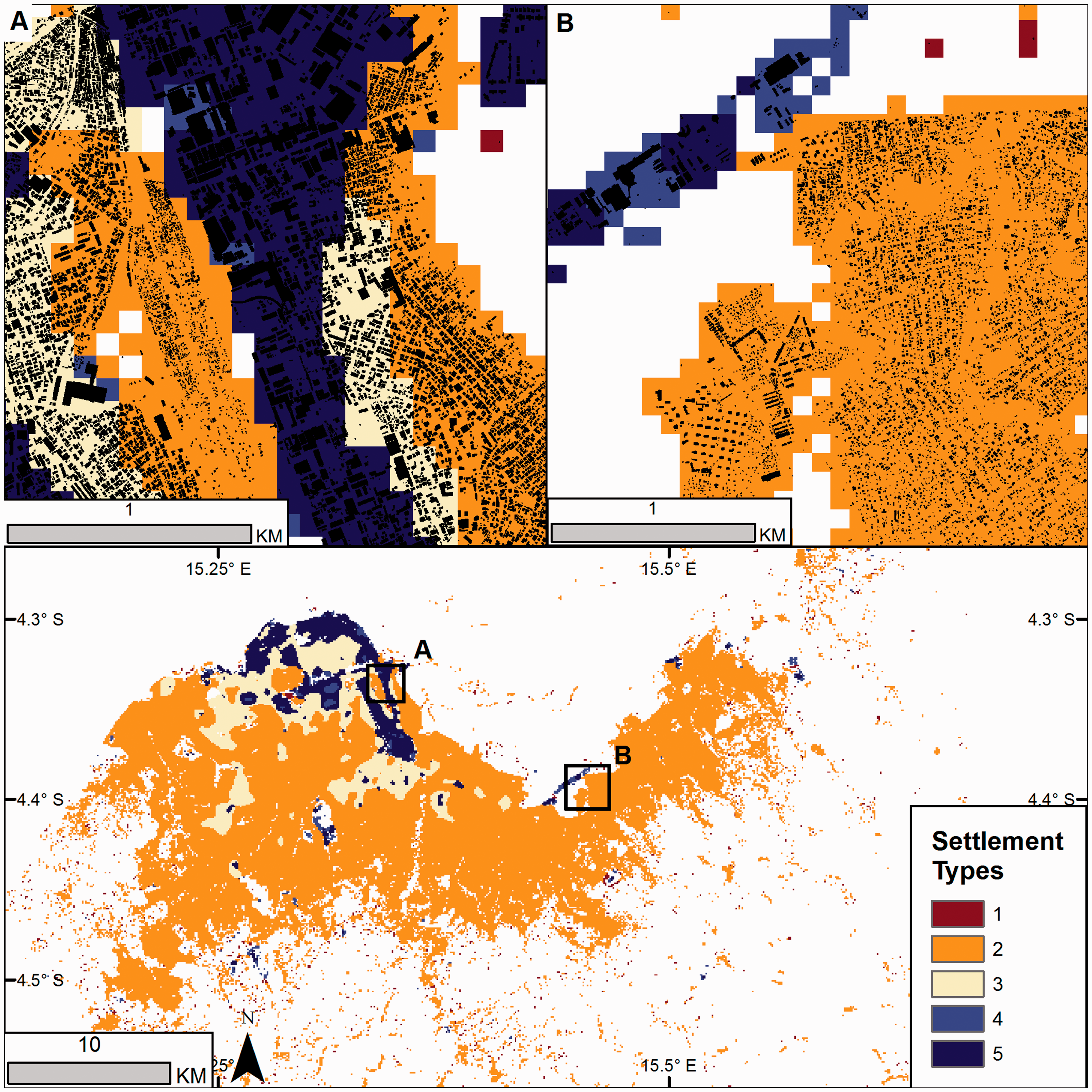
Predicted settlement types for Kinshasa, Democratic Republic of the Congo, at 100 m spatial resolution after merging components. The mixture model components from a 12 settlement type solution were merged to a 5 settlement type solution to reduce entropy in the predicted classes. A 3 × 3 majority smoothing filter was applied to the predicted classes. Examples of the building footprints are shown in the inset maps (a) and (b) overlaid on the predicted types. Settlement types were relabelled by decreasing average patch density after merging. Whitespace in the maps are unsettled pixels.

The Kinshasa study area presents an opportunity to compare our unsupervised clustering results to labelled data. Using a previously published land use map (Bédécarrats et al., 2016; Groupe Huit and Arter, 2014), rasterised to match our predicted settlement type grids, we compared our model-based settlement types at the pixel level. The classification comparison is shown in Figure 5, with the land use classes in the left column mapped to the 5 and 12 predicted settlement types in the right columns, and summarised in Table 1. The land use map was produced in 2014 by planners working with the city government and stakeholders to indicate the main function of areas of the city. The updated map classifies the majority of land in Kinshasa as different residential uses, which reflect changes in the region’s history as Democratic Republic of the Congo gained independence and Kinshasa grew. Planned neighbourhoods and upper class residential areas are more compact, defined, and tend to follow gridded street layouts near the city centre. The self-built housing category occupies the largest land area and more recent areas of growth and expansion on the edges of the city.

Figure 5.

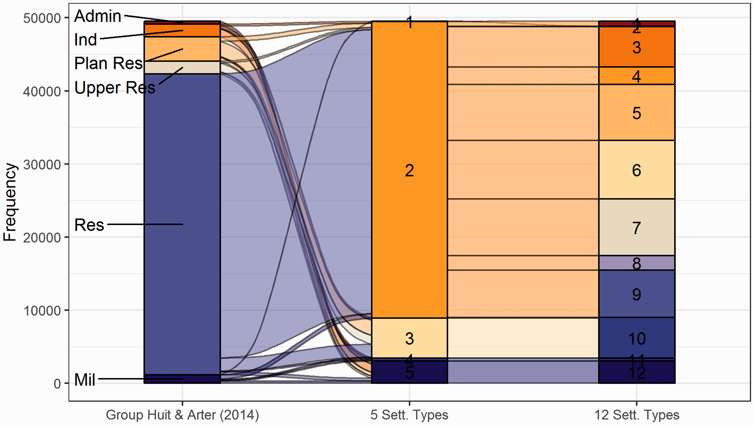
Cross-comparison of a land use map (Groupe Huit and Arter, 2014) with predicted settlement types in Kinshasa at the 100 m pixel level. The land use types include administrative (“Admin”), industrial zones (“Ind”), planned residential neighbourhood (“Plan Res”), upper class residential (“Upper Res”), self-built residential (“Res”), and military camps (“Mil”). Smaller land use types are omitted for clarity. Colours match Figures 3 and 4 for the predicted settlement type maps.

Table 1.

Pixel-level tabulation comparing the Kinshasa land use map classes (Groupe Huit and Arter, 2014) with the five class predicted types from the model-based unsupervised classification method based on building footprint morphology.

	Land use map classes
	Administrative		Industrial		Planned neighbourhood		Upper class residential		Self-built residential		Military		Total
	N	(%)	N	(%)	N	(%)	N	(%)	N	(%)	N	(%)	N
Unsupervised classification
1	0	0.0	0	0.0	0	0.0	0	0.0	26	0.1	34	2.7	60
2	0	0.0	285	16.0	621	18.5	279	15.4	38,874	94.3	637	50.0	40,696
3	0	0.0	285	16.0	2100	62.7	1225	67.6	1799	4.4	118	9.3	5527
4	0	0.0	78	4.4	91	2.7	0	0.0	117	0.3	166	13.0	452
5	393	100.0	1131	63.6	539	16.1	309	17.0	405	1.0	319	25.0	3096
Total	393	100	1779	100	3351	100	1813	100	41,221	100	1274	100

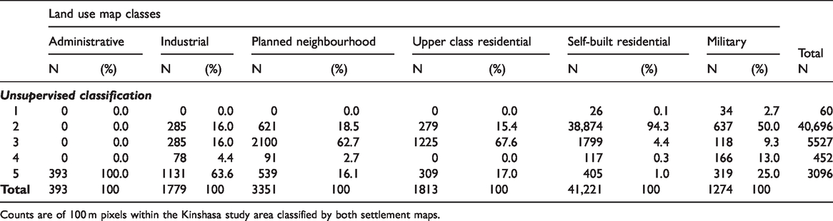
Counts are of 100 m pixels within the Kinshasa study area classified by both settlement maps.

The self-built residential type (labelled in the figure as “Res”) maps on to class 2 of our 5 type classification, which is covered by 7 of the 12 class predicted types. Thus, the settlement pattern-derived types are suggesting additional areas of settlement types within the city land use map. Interestingly, the planned (“Plan Res”) and the upper class (“Upper Res”) residential land use areas are mapped by classes 3 (and 10) of the 5 (and 12) class predicted settlement types, suggesting that they do exhibit morphological patterns that are distinct from most of the other residential lands. The industrial and administrative areas are primarily predicted into type 5 (and type 12) along with military camps. While these areas are clearly distinct from residential uses, the landscape metrics are not able to differentiate between them.

Discussion

Patterns of settlement, location, and configurations are the result of long-term political and economic decisions interacting with the landscape (Seto et al., 2010), but they can reflect differences in the current conditions and help identify areas such as “slums” for targeted interventions (Kuffer et al., 2016). Fragmentation statistics have proven to be able to quantify urban morphology and help to characterise urban areas (Seto and Fragkias, 2005; Seto et al., 2010), but most studies have been conducted at macroscales using land cover maps. Notably, Benza et al. (2016) used fragmentation metrics of vegetation and settlement with decision trees to classify areas around Accra, Ghana, into an urban gradient with a 450 m spatial resolution, though they did not consider multiple spatial scales in their analyses.

Creating settlement type maps that can highlight intra-urban variations while also consistently covering large study areas to facilitate inter-city comparisons remains a challenge. Such classification maps can help monitor urban growth and development and contribute to estimating population size and characteristics (Benza et al., 2017; Grippa et al., 2019). Much attention within urban analytics has been given to making more automated machine learning and processing of new data streams in urban settings (Ibrahim et al., 2019; Yan et al., 2019). These approaches have the advantage of rapidly identifying generalisable patterns within data, but they can face a challenge from inconsistent definitions or understandings of settlement types (Lilford et al., 2019). Our approach to classification is also data-driven, clustering morphological patterns, though rather than emphasising the generalisability of the classifications, we feel it can be best used as part of “complementary technologies” (Engin et al., 2019) with local stakeholder knowledge and guided by an application.

Improvements in image processing are now enabling complete and spatially detailed maps of building footprints to be extracted from VHR imagery for large areas. These buildings create spatial patterns on the landscape. We draw on psychological principles of visual organisation (Li et al., 2004) and leverage high-performance computing resources to quantify urban morphology (size, density, and shape of structures) for local areas. We applied a data sampling and model comparison approach for model-based clustering (Wehrens et al., 2004). Repeated trials of this strategy showed that it provided a balance between consistent results and reduced computational burden. In all three study areas, the model-based clustering approach suggested a large number of variably sized and oriented components. We sought to reduce these model components by merging them to a more easily interpretable number of clusters to predict settlement types. Merging mixture components is a common challenge in model-based clustering (Hennig, 2010). After creating a hierarchy of potential merges based on an entropy score (Baudry et al., 2010), we presented results from two clusterings using the maximum number of components and one that minimised the entropy in the clustering.

The large number of components (11–13) initially identified in the model-based clustering makes it difficult to interpret the results as meaningful settlement types, and the reduced set of clusters suggested by the merging steps can potentially remove important variations. The loss of variation was most noticeable in Kaduna, where large urban areas in the merged results were differentiated primarily into small structures versus large. However, the reduced clustering in Kinshasa and Maputo retained more variation between settlement types in the urban areas. This result may reflect actual differences in the structure of the cities or in the study areas – Kaduna is the largest geographic area, and even though it contains a major city of Northern Nigeria, most of the region is sparsely built up rural areas, while the Kinshasa and Maputo study areas are smaller in extent and focused on large cities. Therefore, an application focused on urban fringes or other particular areas may need to use other criteria to select an optimal clustering solution. In all three study areas, the fringes of the cities were found to contain many settlement types. Benza et al. (2016) note that urban context can best be conceptualised as a gradient based on the degree of built settlement. The different cluster types we found along the edges of the study cities may reflect the model attempting to resolve that transition in urban gradient.

Our comparison with an existing land use map in Kinshasa demonstrates how our unsupervised classification approach can be used in conjunction with other data of a place. While the morphology-based classification maps to the broad categories in the land use map, it can also suggest variations within residential areas. Thus, the clustering solutions can be exploratory and suggest other settlement typologies. Rather than seeking a single, standard definition for supervised classification of settlement types, land uses may be best understood through a combination of on-the-ground knowledge of local contexts with top-down models and data analyses (Mahabir et al., 2016). Baudry et al. (2010) similarly note that a substantive interpretation of clusters should be used as a guide along with methods such as entropy scores. In this way, the hierarchy of clustering outcomes we demonstrate could support a more participatory approach to classifying settlement types by first identifying potential patterns in the data and then enabling people with local knowledge to group them to support particular policy analyses or for relevance in a specific context.

Our work has shown potential to detect and classify settlement patterns in limited, polygon representations of buildings with a few simple metrics; however, we have only tested this approach in three areas of Africa. We have treated the three study areas separately in this work. Urban settlement growth is taking different paths around the world (Schneider et al., 2015), and more work is needed, particularly in the design of training samples, to ensure that the classifications can be generalisable to other places. There is a large number of potential landscape fragmentation statistics (McGarigal, 2015). We have only tested seven metrics that seek to quantify principles of Gestalt theory (Li et al., 2004; Steiniger et al., 2008) and which showed good results in other studies. Future work should examine settlement patterns in other areas and explore if different contexts require certain metrics. We also note that this work has only used landscape metrics that can be calculated from the building footprint patterns. Our goal was not to include any other data, though a possible extension to the work could consider patterns of vegetation as Benza et al. (2016) did, or include other features such as roads, major intersections, or points-of-interest to help characterise settlement types.

The resolution of the classification maps should be explored further. These analyses have used an approximately 100 m resolution grid in order to create classification maps which integrate with other openly available demographic and geospatial datasets (e.g., Lloyd et al., 2019). However, this resolution may be too coarse to detect local changes in morphology in dense urban areas. On the other hand, a very fine resolution classification with more local variation between settlement types may be difficult to interpret, particularly in sparsely settled areas. The choice of processing resolution should ultimately be guided by the application or research question.

An important consideration in this approach to classifying settlement areas is the accuracy of the building footprint dataset. We used a commercial dataset for this work, but other datasets could potentially be used in similar analyses, though all would face similar issues if there is incompleteness. While OpenStreetMap shows variable completeness in digitised buildings (Hecht et al., 2013), in areas with adequate coverage, it could provide an alternative source. Additionally, the Microsoft-produced building footprints have recently become openly available for Tanzania and Uganda (https://github.com/microsoft/Uganda-Tanzania-Building-Footprints). This growing availability of such building datasets will hopeful encourage other creative uses of such data to study urban areas.

Conclusion

As urban settlements continue to grow in size and in population, understanding their differences, both within and between cities, becomes key for planning, delivering, and monitoring projects in support of sustainable development. While future cities are often envisioned as a web of interconnected systems and both generating and supported by a wealth of new data streams, in many parts of the world, information on basic city structure and function is still lacking or non-existent. This data gap is particularly acute in low- and middle-income countries, many of which are experiencing the fastest urban transitions. Advances in VHR imagery and remote sensing data, along with improved computational power, are helping to provide information on urban areas through building feature extractions. This work provides an example of how computational methods can be used to extract new information from such big geospatial datasets to support research on population and development.

Supplemental Material

sj-pdf-1-epb-10.1177_2399808320921208 - Supplemental material for Classifying settlement types from multi-scale spatial patterns of building footprints

Supplemental material, sj-pdf-1-epb-10.1177_2399808320921208 for Classifying settlement types from multi-scale spatial patterns of building footprints by Warren C Jochem, Douglas R Leasure, Oliver Pannell, Heather R Chamberlain, Patricia Jones and Andrew J Tatem in Environment and Planning B: Urban Analytics and City Science

Footnotes

Acknowledgements

The authors acknowledge the use of the IRIDIS Higher Performance Computing Facility, and associated support services at the University of Southampton, in the completion of this work.

Declaration of conflicting interests

The author(s) declared no potential conflicts of interest with respect to the research, authorship, and/or publication of this article.

Funding

The author(s) disclosed receipt of the following financial support for the research, authorship, and/or publication of this article: This work was conducted as part of the Geo-Referenced Infrastructure and Demographic Data for Development project (GRID3; OPP1182408) funded by the Bill & Melinda Gates Foundation and the United Kingdom’s Department for International Development.

Warren C Jochem is a Senior Research Fellow with WorldPop in the School of Geography and Environmental Science at the University of Southampton. His work focuses on developing and applying computational and spatial statistical methods to study the distribution, dynamics, and health of populations.

Douglas R Leasure is a Research Fellow with WorldPop in the School of Geography and Environmental Science at the University of Southampton. His work focuses on the development of statistical methods for high-resolution population mapping using limited survey data.

Oliver Pannell is a GIS technician with WorldPop in the School of Geography and Environmental Science at the University of Southampton. His recent work is on harmonising and analysing geospatial datasets to support several projects on spatial demography and vaccination coverage mapping.

Heather Chamberlain is an Enterprise Fellow with WorldPop in the School of Geography and Environmental Science at the University of Southampton. She has a background in GIS and remote sensing and her work focuses on integrating geospatial datasets for population estimation and high-resolution mapping of sociodemographics.

Patricia Jones is a GIS technician with WorldPop in the School of Geography and Environmental Science at the University of Southampton. Her recent work is on integrating and analysing geospatial datasets to support several projects on high-resolution population and settlement mapping.

Andrew J Tatem is Professor of Spatial Demography and Epidemiology in the School of Geography and Environmental Science and Director of WorldPop at the University of Southampton and the Flowminder Foundation. His recent work is focused on the application of spatial demographics in malaria burden estimation, maternal and newborn health and poverty mapping, as well as the dispersal of diseases and their vectors through global transport networks and quantifying population movements in relation to disease dynamics.

ORCID iD

Oliver Pannell

Supplemental material

Supplemental material for this article is available online.

References

Barr

Barnsley

Steel

(2004) On the separability of urban land-use categories in fine spatial scale land-cover data using structural pattern recognition. Environment and Planning B: Planning and Design 31: 397–418.

Baudry

Raftery

Celeux

, et al. (2010) Combining mixture components for clustering. Journal of Computational and Graphical Statistics : A Joint Publication of American Statistical Association, Institute of Mathematical Statistics, Interface Foundation of North America 9: 332–353.

Bédécarrats

Lafuente-Sampietro

Leménager

, et al. (2016) Building commons to cope with chaotic urbanization? Performance and sustainability of decentralized water services in the outskirts of Kinshasa. Journal of Hydrology 573: 1096–1108.

Benza

Weeks

Stow

, et al. (2016) A pattern-based definition of urban context using remote sensing and GIS. Remote Sensing of Environment 183: 250–264.

Benza

Weeks

Stow

, et al. (2017) Fertility and urban context: A case study from Ghana, West Africa, using remotely sensed imagery and GIS. Population, Space and Place 23: e2062.

Biernacki

Celeux

Govaert

(2000) Assessing a mixture model for clustering with the integrated completed likelihood. IEEE Transactions on Pattern Analysis and Machine Intelligence 22: 719–725.

Bing Maps Team (2018) Microsoft releases 125 million building footprints in the US as open data. Available at: https://blogs.bing.com/maps/2018-06/microsoft-releases-125-million-building-footprints-in-the-us-as-open-data (accessed 11 April 2020).

Bing Maps Team (2019) Microsoft releases 12 million Canadian building footprints as open data. Available at: https://blogs.bing.com/maps/2019-03/microsoft-releases-12-million-canadian-building-footprints-as-open-data (accessed 11 April 2020).

Bogaert J, Van Hecke P, Eysenrode D, et al. (2000) Landscape Fragmentation Assessment Using a Single Measure. Wildlife Society Bulletin (1973--2006) 28(4): 875--881.

10.

Cheriyadat

Bright

Potere

, et al. (2007) Mapping of settlements in high-resolution satellite imagery using high performance computing. GeoJournal 69: 119–129.

11.

DigitalGlobe (2018) Data sheet: Ecopia building footprints powered by DigitalGlobe. Available at: https://dgv4-cms-production.s3.amazonaws.com/uploads/document/file/67/DG_Building_Footprints_DS_08-2018_.pdf (accessed 17 April 2020)

12.

Ecopia and DigitalGlobe (2017) Technical specification: Ecopia building footprints powered by DigitalGlobe. Available at: https://dg-cms-uploads-production.s3.amazonaws.com/uploads/legal_document/file/109/DigitalGlobe_Ecopia_Building_Footprints_Technical_Specification.pdf (accessed 11 April 2020).

13.

Engin

van Dijk

Lan

, et al. (2019) Data-driven urban management: Mapping the landscape. Journal of Urban Management. Available at: https://doi.org/10.1016/j.jum.2019.12.001.

14.

Engstrom

Sandborn

, et al. (2015) Mapping Slums Using Spatial Features in Accra, Ghana: Joint Urban Remote Sensing Event (JURSE). Lausanne, Switzerland: IEEE.

15.

Fraley

Raftery

(2003) Enhanced model-based clustering, density estimation, and discriminant analysis software: MCLUST. Journal of Classification 20: 263–286.

16.

Graesser

Cheriyadat

Vatsavai

, et al. (2012) Image based characterization of formal and informal neighborhoods in an urban landscape. IEEE Journal of Selected Topics in Applied Earth Observations and Remote Sensing 5: 1164–1176.

17.

Grippa

Linard

Lennert

, et al. (2019) Improving urban population distribution models with very-high resolution satellite information. Data 4: 13.

18.

Groupe Huit and Arter (2014) Schéma D’Orientation Stratégique De L’Agglomération de Kinshasa (SOSAK) et Plan Particulier D’Aménagement de la Partie Nord de la Ville (PPA): Gouvernement Provincial de la Ville de Kinshasa. Available at: https://www.kinshasa2030.net/publications. (accessed 3 March 2019)

19.

Hecht

Kunze

Hahmann

(2013) Measuring completeness of building footprints in OpenStreetMap over space and time. ISPRS International Journal of Geo-Information 2: 1066–1091.

20.

Hecht

Meinel

Buchroithner

(2015) Automatic identification of building types based on topographic databases – A comparison of different data sources. International Journal of Cartography 1: 18–31.

21.

Hennig

(2010) Methods for merging gaussian mixture components. Advances in Data Analysis and Classification 4: 3–34.

22.

Ibrahim

Titheridge

Cheng

, et al. (2019) predictSLUMS: A new model for identifying and predicting informal settlements and slums in cities from street intersections using machine learning. Computers, Environment and Urban Systems 76: 31–56.

23.

Irwin

Bockstael

(2007) The evolution of urban sprawl: Evidence of spatial heterogeneity and increasing land fragmentation. Proceedings of the National Academy of Sciences of the United States of America 104: 20672–20677.

24.

Jochem

Bird

Tatem

(2018) Identifying residential neighbourhood types from settlement points in a machine learning approach. Computers, Environment and Urban Systems 69: 104–113.

25.

Kit

Lüdeke

Reckien

(2012) Texture-based identification of urban slums in Hyderabad, India using remote sensing data. Applied Geography 32: 660–667.

26.

Kuffer

Barros

Sliuzas

(2014) The development of a morphological unplanned settlement index using very-high-resolution (VHR) imagery. Computers, Environment and Urban Systems 48: 138–152.

27.

Kuffer

Pfeffer

Sliuzas

(2016) Slums from space—15 years of slum mapping using remote sensing. Remote Sensing 8: 455.

28.

Yan

, et al. (2004) Automated building generalization based on urban morphology and gestalt theory. International Journal of Geographical Information Science 18: 513–534.

29.

Lilford

Kyobutungi

Ndugwa

, et al. (2019) Because space matters: Conceptual framework to help distinguish slum from non-slum urban areas. BMJ Global Health 4:

30.

Lloyd

Chamberlain

Kerr

, et al. (2019) Global spatio-temporally harmonised datasets for producing high-resolution gridded population distribution datasets. Big Earth Data 3: 108–139.

31.

Luck

(2002) A gradient analysis of urban landscape pattern: A case study from the phoenix metropolitan region, Arizona, USA. Landscape Ecology 17: 327–339.

32.

Lüscher

Weibel

(2013) Exploiting empirical knowledge for automatic delineation of city centres from large-scale topographic databases. Computers, Environment and Urban Systems 37: 18–34.

33.

Mahabir

Crooks

Croitoru

, et al. (2016) The study of slums as social and physical constructs: Challenges and emerging research opportunities. Regional Studies, Regional Science 3: 399–419.

34.

McDonald

Kareiva

Forman

(2008) The implications of current and future urbanization for global protected areas and biodiversity conservation. Biological Conservation 141: 1695–1703.

35.

McGarigal

(2015) FRAGSTATS help. Available at: http://www.umass.edu/landeco/research/fragstats/documents/fragstats.help.4.2.pdf (accessed 11 April 2020).

36.

McGarigal

Tagil

Cushman

(2008) Surface metrics: An alternative to patch metrics for the quantification of landscape structure. Landscape Ecology 24: 433–450.

37.

McLachlan

Rathnayake

(2014) On the number of components in a Gaussian mixture model. Wiley Interdisciplinary Reviews: Data Mining and Knowledge Discovery 4: 341–355.

38.

McNicholas

(2016) Model-based clustering. Journal of Classification 33: 331–373.

39.

Patlolla

Bright

Weaver

, et al. (2012) Accelerating satellite image based large-scale settlement detection with GPU. In: SIGSPATIAL 2012 International Conference on Advances in Geographic Information Systems, Redondo Beach California, November, 2012. ACM 43–51. Available at: https://doi.org/10.1145/2447481.2447487.

40.

R Core Team (2017) R: A Language and Environment for Statistical Computing. Vienna, Austria: R Foundation for Statistical Computing, Available at: https://www.-R-project.org (accessed 11 April 2020).

41.

Rosser

Boyd

Long

, et al. (2019) Predicting residential building age from map data. Computers, Environment and Urban Systems 73: 56–67.

42.

Roy Chowdhury

Bhaduri

McKee

(2018) Estimating urban areas: New insights from very high-resolution human settlement data. Remote Sensing Applications: Society and Environment 10: 93–103.

43.

Schneider

Mertes

Tatem

, et al. (2015) A new urban landscape in East–Southeast Asia, 2000–2010. Environmental Research Letters 10: 034002.

44.

Schneider

Woodcock

(2008) Compact, dispersed, fragmented, extensive? A comparison of urban growth in twenty-five global cities using remotely sensed data, pattern metrics and census information. Urban Studies 45: 659–692.

45.

Scrucca

(2016) Identifying connected components in Gaussian finite mixture models for clustering. Computational Statistics & Data Analysis 93: 5–17.

46.

Scrucca

Fop

Murphy

, et al. (2016) mclust5: Clustering, classification and density estimation using Gaussian finite mixture models. The R Journal 8: 289–317.

47.

Seto

Fragkias

(2005) Quantifying spatiotemporal patterns of urban land-use change in four cities of China with time series landscape metrics. Landscape Ecology 20: 871–888.

48.

Seto

Sánchez-Rodríguez

Fragkias

(2010) The new geography of contemporary urbanization and the environment. Annual Review of Environment and Resources 35: 167–194.

49.

Steiniger

Lange

Burghardt

, et al. (2008) An approach for the classification of urban building structures based on discriminant analysis techniques. Transactions in GIS 12: 31–59.

50.

Taubenböck

Esch

Felbier

, et al. (2012) Monitoring urbanization in mega cities from space. Remote Sensing of Environment 117: 162–176.

51.

UN Department of Economic and Social Affairs (2019) World population prospects: Highlights. Available at: https://population.un.org/wpp/Publications/Files/WPP2019_Highlights.pdf (accessed 11 April 2020).

52.

UN General Assembly (2017) New Urban Agenda: Res: 71/256. New York: United Nations.

53.

UN Habitat (2016) Urbanization and Development: Emerging Futures. Nairobi, Kenya: UN Habitat.

54.

Wardrop

Jochem

Bird

, et al. (2018) Spatially disaggregated population estimates in the absence of national population and housing census data. Proceedings of the National Academy of Sciences of the United States of America 115: 3529–3537.

55.

Wehrens

Buydens

LMC

Fraley

, et al. (2004) Model-based clustering for image segmentation and large datasets via sampling. Journal of Classification 21: 231–253.

56.

WHO and UN-Habitat. (2010) Hidden Cities: Unmasking and Overcoming Health Inequities in Urban Settings. Switzerland: WHO and UN-Habitat.

57.

Yan

Yang

, et al. (2019) A graph convolutional neural network for classification of building patterns using spatial vector data. ISPRS Journal of Photogrammetry and Remote Sensing 150: 259–273.

58.

Yuan

(2016) Automatic building extraction in aerial scenes using convolutional networks. arXiv preprint arXiv:1602.06564.

59.

Yuan

Wang

Cheriyadat

(2015) Factorization-based texture segmentation. IEEE Transactions on Image Processing: A Publication of the IEEE Signal Processing Society 24: 3488–3497.

Supplementary Material

Please find the following supplemental material available below.

For Open Access articles published under a Creative Commons License, all supplemental material carries the same license as the article it is associated with.

For non-Open Access articles published, all supplemental material carries a non-exclusive license, and permission requests for re-use of supplemental material or any part of supplemental material shall be sent directly to the copyright owner as specified in the copyright notice associated with the article.

0.00 MB

3.65 MB