Sage Journals: Discover world-class research

Abstract

Background. COVID-19 tremendously disrupted the global health system. People of all ages were at risk of becoming infected. Frequent school closures raised concerns about both the physical and mental health of school-age children. Many studies discussed the effectiveness of various interventions, while few focused on optimizing such interventions. Methods. This study aimed to optimize the usage of random screening tests and masking requirements within K-12 schools. We simulated the disease transmission within a school setting and sought to find the most efficient schedules for schools to arrange their weekly screening tests and mask mandates. The goal was to minimize the number of the end-of-semester infections as well as to use the minimum number of resources. We applied the nondominated sorting genetic algorithm, NSGA-II, to solve this multiobjective optimization problem. We also compared results when polymerase chain reaction (PCR) versus rapid antigen tests were used. Results. The NSGA successfully found Pareto solutions when optimizing the end-of-semester infections, the total number of tests, and the total number of weeks masking. The screening tests and masks can serve as alternatives to one another when prioritizing minimizing the number of infections. In addition, due to the faster return of testing results and lower accuracy, the rapid antigen tests had a similar effect as PCR tests. Conclusion. Our study provides policy makers in K-12 schools with valuable insights. The conclusions derived from this research can serve as a solid foundation for making informative decisions regarding random screening tests and universal masking policies.

Highlights

Our simulation optimization framework was used to design weekly schedules for random screening tests and masking within K-12 schools to mitigate COVID-19 infections.

We considered multiple objectives and applied the NSGA-II algorithm to find a Pareto solution set.

Based on local context and preferences, decision makers can trade off testing and masking to achieve a similar number of end-of-semester infections.

When a few weeks of masks are mandated, it is best to use them at the beginning of a semester.

Keywords

SEIR model simulation optimization infectious disease in-school testing masking

COVID-19 has posed great challenges to the global health system since 2020. This airborne, highly transmissive disease was responsible for causing more than 103 million cases and more than 1 million deaths as of December 2023.¹

It is well documented that hospitalization rates for individuals infected with COVID-19 vary by age, with significantly higher rates for people who are 65 y and older (511.9 per 100,000) compared with 5- to 17-y-olds (21.4 per 100,000) based on data from the beginning of January 2022.² Because of this, many studies regarding the effectiveness and design of nonpharmaceutical interventions (NPIs) focused on the general population or older adults.^3,4 However, children contribute significantly to infections.⁵ It was estimated that about 9.8% of infections originated from children aged 0 to 19 y when schools reopened in October 2020, which is much higher than the proportion of infections originating from those 65 y and older (about 2.8%) due to the different social dynamics among different age groups. Thus, analyzing disease transmission among younger age groups within the school environment is important, not only for disease control among school-aged children but also for protecting the entire community.⁶

During 2020 to 2023, many different interventions were implemented in K-12 schools (the term “K-12 schools” is commonly used in the United States to represent primary and secondary education from kindergarten to 12th grade). In previous work,⁷ we demonstrated the effectiveness of NPIs, such as universal masking, random screening tests, and school closures. However, there may be some negative consequences associated with implementing NPIs, such as school closures. For example, it is estimated that more than 370 million children lost access to their primary source of balanced and nutritious meals when schools were shut down during the pandemic.⁸ Furthermore, children experienced significant learning loss due to school closures during the pandemic.⁹ Parents were also worried about their children’s lack of social and physical activities, which may affect their social and emotional well-being and lead to mental health issues such as anxiety and depression.^10,11 Data show that from April to October 2020, among all pediatric ED visits, the proportion of mental health–related ED visits increased by more than 20% for children from 5 to 17 y old.¹² Thus, in this article, we excluded school closures as a potential NPI and examined how we can keep children in school and at the same time keep them safe through the use of other NPIs.

In 2022, pandemic fatigue rose, and opposition to wearing masks grew.¹³ In early 2022, mask mandates were lifted in most K-12 schools that had implemented them.¹⁴ Most schools also stopped requiring negative test results after illness, removed partitions between seats, and brought back regular school events and activities. However, the highly contagious subvariant of Omicron brought new challenges to K-12 schools in late 2022 and early 2023, which resulted in some school districts reimplementing mask mandates and other preventive measures after winter break.¹⁵ During that time, state-funded testing programs were proposed by the North Carolina Department of Health and Human Services, which allowed schools in North Carolina to determine their preferred testing/quarantine and isolation plan.¹⁶ Montgomery County Public Schools (MCPS) in Maryland stated that they would implement COVID-19 mitigation strategies in their Spring 2023 Reopening Guide. Some of the strategies included strategically timed screening tests, testing following school-based outbreaks, and using face coverings to maintain safe in-person learning.¹⁷ These events suggested that interventions were still necessary in schools but needed to be implemented in a way that considered the local context and preferences.

Policy planning and resource allocation are essential for improved preventive health. In uncertain and complex environments, the integration of simulation and optimization techniques can be an effective approach to aid decision makers. The results from these tools can provide guidance for stakeholders to reduce the burden of disease when resources are limited. In this work, we focused on helping K-12 schools find the best way to utilize and allocate the NPIs, such as tests and masks, which schools can easily access. Therefore, we designed and solved a multiobjective simulation optimization problem within a school setting, with the goal of finding an optimal solution for K-12 schools to plan their random screening tests and universal masking schedules while minimizing end-of-semester infections. While the results provided are based on the COVID-19 pandemic, this framework can easily be extended to future pandemics.

Methods

In this section, we briefly discuss the design of the multigrouped susceptible-exposed-infected-recovered (SEIR) model we built in a previous study.⁷ Due to the rapid mutation of the Omicron subvariants, we made the necessary modifications and parameterizations to the previous model. The full list of parameters is provided in the appendix. We also describe in detail the design of the optimization problem as well as the assumptions we made.

Simulation Model Structure and Parameters

In 2022, we built a multigrouped SEIR model to simulate the disease transmission within US K-12 schools using R programming language. For the model structure, we considered 9 different health states, as shown in Figure 1. In the model, we broke down the “infected” states into asymptomatic (“Infected(A)”), presymptomatic (“Infected(pre-S)”), and symptomatic (“Infected(S)”). We also distinguished the posttesting states based on the testing results and isolation status. Because COVID-19 tests can be inaccurate under certain circumstances, we considered the possibility of false negatives, followed by the “recovered unknown” state. All the individuals exclusively belonged to one of the health states at any point during the simulation.

Figure 1

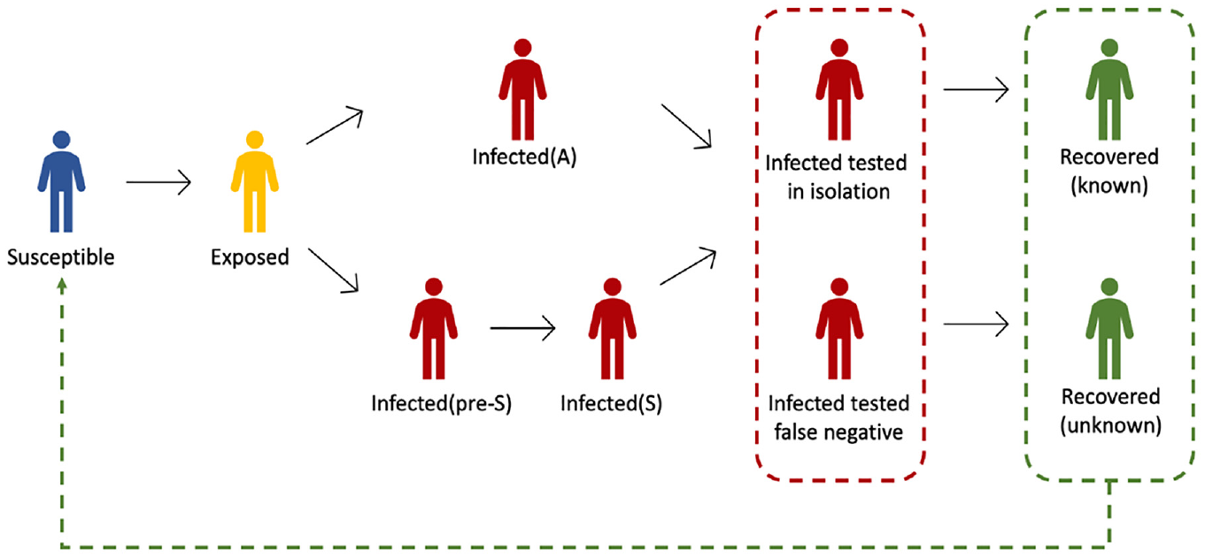
Flowchart of the updated COVID-19 disease model.

To keep up with the newest subvariant of COVID-19 and to find the optimal schedule, we made several modifications to the original model. First, the subvariant BA.5 was highly contiguous and responsible for a high reinfection rate. We assumed the reinfection rate was 13%,¹⁸ and the time between “recovered” and “susceptible” had a mean of 100 d.¹⁹ Thus, in addition to the general flow of susceptible-exposed-infected-recovered, we included the transition from “recovered” to “susceptible,” as shown by the green dotted line in Figure 1. In the simulation, we assumed the isolation compliance rate after a school-based positive test to be 100%. Then, infected individuals who received tests would be either positive and isolated or false negative. The differential equations associated with the model are described in the appendix, and the R code is shared in a GitHub repository (https://github.com/yz-ncsu/Optimizing-Masks-and-Random-Screening-Test-Usage-within-K-12-Schools).

With regard to the multigrouped model setting, we split the students and teachers within the school into subgroups and parameterized 3 distinct contact matrices to represent different social patterns within elementary schools (K-5), middle schools, and high schools. For K-5, we assumed the total population of students and teachers was 500, with a total of 18 student subgroups and a teacher subgroup. The 3 contact patterns were “well-mixed,”“cohort,” and “isolated.”“Cohort” represented the social-distancing strategy during the pandemic, in which students had close to a prepandemic-level interaction within their own classrooms but fewer interactions outside of their subgroups. The contact matrices for the different contact patterns are included in the appendix. In this study, we assumed students and teachers were “well-mixed,” representing the schools returning to prepandemic classroom spacing. In addition, although the model was capable of simulating K-12 schools, we limited our analysis to K-5 in this study. In addition, we assumed 1 of the 500 individuals was exposed on the first day of the semester. For the rest of the individuals, 30% of the K-5 school students and 50% of the teachers were in the “recovered” state due to vaccination or previous infection.

We also introduced the concept of weekdays and weekends in the simulation. We assumed the transmission rate within schools was zero during the weekends, as there was no interaction between individuals in schools. The overall simulation period was 107 d, which was about the length of a semester, and the first day of school was assumed to be Monday.

We considered the disease burden from the community by simulating a dynamic disease prevalence during the semester. We generated a random variable $Y_{i} ~ {\begin{matrix} DU [3, 4], i \leq 4 \\ DU [1, 2], i \geq 5 \end{matrix}$ , representing the number of newly exposed individuals whose exposure occurred from outside of school in week $i$ , following a discrete uniform distribution. We assumed the disease burden from the community was higher in the first weeks when schools reopened, as studies have shown that an increase in COVID-19 cases is associated with the opening of K-12 schools in the United States.²⁰

Design of the Optimization Problem

Layered on top of the simulation model, we designed a multiobjective optimization problem. We treated the number of the end-of-semester infections (this includes infections acquired in and outside of the school), the number of random screening tests, and weeks of masks as our 3 objectives. We aim to solve the problem by minimizing all 3 of the objectives together.

There were 2 sets of decision variables in this problem: the testing ratio and the mask usage each week. We considered the testing ratio in each week $X_{1} = X_{1, 1}, \dots, X_{1, j}, \dots, X_{1, 16}$ as the first set of decision variables in the problem. The possible test ratios for schools to consider were 0%, 20%, 40%, 60%, and 80%. If $X_{1, j} = 20 %$ , it means 20% of the individuals who are present in school will be randomly selected to get tested in week $j$ . Alternatively, if $X_{1, j} = 0 %$ , it means no screening tests will be performed in week $j$ . We call this testing schedule $X_{1}$ planned testing. In addition, the school can also determine whether to implement universal masking each week. Mask usage was treated as a set of binary variables. Note that the effectiveness of masks was hard to estimate due to the different materials or proper usage (e.g., over mouth and nose). Thus, we made our assumption about the effectiveness of masks based on the combination of efficacy and adherence.²¹ If masks were used, we assumed the effectiveness of masks was 25% during that week, which was calculated by multiplying the mask efficacy of 50% by the mask adherence level of 50%. Thus, we defined an additional group of decision variables: $X_{2} = X_{2, 1}, \dots, X_{2, j}, \dots, X_{2, 16}$ . $X_{2, j}$ are binary variables, representing whether or not mask usage is recommended during week $j$ .

The formulation of the 3-objective optimization problem is shown below. In the formulation, $C_{1}$ is the number of end-of-semester infections within the school and $C_{2}$ is the number of random screening tests performed. The third cost function $C_{3}$ is the number of weeks masks are used, which is equal to $\sum_{j = 1}^{16} X_{2, j}$ . The solutions to this problem will contain a set of $X_{1}$ and $, X_{2}$ , which indicate the desired testing ratio and mask usage policy each week.

min_{X} F = (C_{1} (X_{1}, X_{2}), C_{2} (X_{1}, X_{2}), C_{3} (X_{1}, X_{2}))

s . t . X_{1, j} \in {0 %, 20 %, 40 %, 60 %, 80 %}

X_{2, j} = {\begin{matrix} 0, & if NO mask usage in week j \\ 1, & otherwise \end{matrix}

j = 1, 2, \dots, 16

(1)

We also considered the dynamic changes in disease transmission during the semester. When the disease starts to spread quickly in a school, many students or teachers may be absent either because they isolate following positive test results or because they develop symptoms and decided to self-quarantine at home. This results in missed school time during the semester. To reduce daily absences, we added the intervention of additional random screening tests, which are triggered by the number of students and teachers who were absent at the beginning of each week. Specifically, if 10 students or 2 teachers are absent on Monday, an additional set of random screening tests at the level of 40% will be scheduled the next day. Because the school population is 500, 10 students correspond to 2% of the school population. We call this absence-triggered (AT) testing; this was designed to simulate the screening tests following school-based outbreaks that the MCPS schools reopen guide suggested.¹⁷

In this study, we assumed the testing kits used in K-12 schools could either be polymerase chain reaction (PCR) tests or rapid antigen tests. The 2 types of testing kits have distinctive characteristics. For instance, rapid antigen tests do not require lab work to retrieve results; thus, results are returned very quickly. PCR tests are much more expensive than rapid antigen tests but more accurate, especially for asymptomatic individuals. The sensitivity rate and specificity rate for PCR tests and rapid antigen tests (symptomatic or asymptomatic) are shown in Table 1.^22–24 The results for the rapid antigen tests and PCR tests are shown separately in the Results section.

Table 1

Sensitivity and Specificity Rate of Polymerase Chain Reaction (PCR) Tests and Rapid Antigen Tests among Symptomatic and Asymptomatic People

	PCR	Rapid Antigen (Symptomatic)	Rapid Antigen (Asymptomatic)
Sensitivity rate, %	89.9	73	54.7
Specificity rate, %	99.9	99.1	99.7

From equation (1), we can see that the 2 sets of decision variables have 5 and 2 possible values, respectively, forming a total number of $5^{16} \times 2^{16}$ potential solutions to the problem. The algorithm we chose to solve the multiobjective minimization problem is the NSGA-II genetic algorithm. This algorithm allows us to treat this problem as a multiobjective optimization problem instead of assigning a specific weight to each of the cost functions. In a single run, the algorithm is able to find a set of optimal solutions called the Pareto front set.

We modified the function “nsga2R” in the R package called “nsga2R” to solve our multiobjective optimization problem.^25,26 There are 4 main parameters of NSGA-II with some conventional choices. Based on the parameter tuning process we conducted in another study, we chose the number of generations = 100, population size = 50, probability of crossover ( $P_{c}$ ) = 0.9, and probability of mutation ( $P_{m}$ ) = 0.03125.²⁷ One simulation run that takes a population of 50 through 100 generations takes approximately 4.35 h. We fixed the initial seeding and conducted analyses based on a single replication of the simulation optimization process. The simulation optimization code is also included in the GitHub repository.

In each iteration (generation), the algorithm sorts the parent and offspring populations, retaining the best solutions from the nondominated set for the subsequent iteration until all iterations are complete. Note that good solutions are sometimes discarded to ensure diversity among the solutions. To ensure this, those with the largest crowding distance are also selected for the next iteration. As a result, within a single simulation run, the algorithm identifies multiple diverse Pareto-optimal solutions. In the appendix (Figure D-2), we provide an example of how the solutions change over iterations to yield a Pareto-optimal solution.

Results

Optimal Solutions: PCR Tests

First, we ran the simulation and solved the problem assuming PCR tests were used as the measure of screening tests in school. Planned testing, if used, was scheduled once per week on Wednesday. By leveraging 3 cost functions in the process of optimization at the same time, we found 47 optimal solutions within the Pareto front, all of which are not dominated by each other. In Figure 2, each dot represents the cost function values $F$ of an optimal solution resulting from a combination of decision variables: screening test ratio and mask usage. For ease of comparison, the optimal solutions with the same level of mask usage are connected with lines. For example, the leftmost brown point represents an optimal objective consisting of 3 parts: 4 wk of masks (as shown by the color), 0 PCR tests, and 278 end-of-semester infections. In other words, if implementing 4 wk of masks without performing any PCR test (x-axis), the lowest number of end-of-semester infections is 278 (y-axis). We can see that there is a downward trend in the scatter plot. That is, under each value of weeks of masks, the number of end-of-semester infections decreases as the number of screening tests increases, illustrated by lines exhibiting negative slopes; under a similar amount of screening tests, more weeks of mask usage result in fewer end-of-semester infections.

Figure 2

The 47 optimal values of the objective in the Pareto front. The y-axis represents the end-of-semester infections (C₁); the x-axis represents the number of random screening tests (C₂); the color of the dots represents the number of weeks of masks during the entire semester (C₃). Same number of weeks of masks are connected with lines. The 7 Pareto solutions marked with red squares are picked as representative solutions for further analysis.

We picked 7 of the Pareto-optimal solutions with end-of-semester values scattered over the limits within the Pareto front to explore further; they are marked with squares in Figure 2 and listed in Table 2. For each of the Pareto-optimal solutions, the columns show the following information: the total end-of-semester infections, the total number of PCR tests performed during the semester, the total number of days when tests occurred (note that this equals the total number of days when the planned testing occurred plus the total number of days when AT testing occurred, as shown in the fifth and sixth columns), and the total number of weeks masks were scheduled. From Table 2, we observe (from the sixth row) that 1 week of masks and 880 screening tests together result in 278 end-of-semester infections. From the fifth row, we see that under a similar level of infections, those 880 screening tests can be saved if 3 more weeks of masks are carried out. In addition, we notice that we can achieve as few as 192 end-of-semester infections if we implement planned testing and masks every week. In addition, we notice that for result 3 and result 6, AT testing occurred twice. This occurred because the daily number of absent students exceeded 10 two times. Although it cannot be observed from Table 2, we point out that AT was not triggered by teacher absences in any of the results shown. We believe this was because of the higher proportion of teachers who were “recovered” prior to the beginning of the semester due to vaccination or prior infection.

Table 2

The 7 Representative Optimal Schedules Picked from the Pareto Front by Ascending Order of Total Infection

Index	Total Infection	Total Number of Tests	Total Number of Test Days (Includes AT Test Days)	Total Planned Testing Days	Total AT Testing Days	Total Weeks of Masks
Result_1	192	6,061	16	16	0	16
Result_2	217	2,474	8	8	0	12
Result_3	245	2,872	9	7	2	6
Result_4	265	3,142	12	9	3	2
Result_5	278	0	0	0	0	4
Result_6	278	880	4	2	2	1
Result_7	292	584	3	0	3	0

AT, absence triggered.

We designed 4 extreme scenarios: “Result_No_Test_No_Mask” means no screening tests or masks are implemented during the entire semester; “Result_Test_All” represents the scenario where the planned testing is scheduled each week with a ratio equal to the maximum value of 80% and assumes AT testing occurs every week as well, but no mask usage is required; “Result_Mask_All” means masks are put in effect every week during the semester but no screening tests, neither planned testing nor AT testing are used; “Result_All_Test_All_Mask” is the scenario of fully implementing both interventions, 80% planned testing, AT testing and mask usage every week. The percentage choice of testing was designed to reflect the highest level of testing in the simulation.

Figures 3 and 4 show the cumulative number of infections and the daily number of infections of the 4 extreme scenarios as well as the 7 representative optimal solutions, respectively. Clearly, “Result_All_Test_All_Mask” returns the lowest number of cumulative infections, but many screening tests and masks are used, which require additional funds and time. On the other hand, no interventions at all “Result_No_Test_No_Mask” resulted in 301 infections in the school by the end of the semester. The cumulative infections of the representative optimal solutions fall strictly between “Result_No_Test_No_Mask” and “Result_All_Test_All_Mask.”

Figure 3

The cumulative number of infections under the 7 representative optimal schedules as well as the 4 extreme scenarios.

Figure 4

The daily number of infections under the 7 representative optimal schedules as well as the 4 extreme scenarios.

In Figure 2, we can see the 3 optimal solutions where universal masking is never implemented (0 wk, as seen by the gray dots). By comparing these 3 solutions in Table 3, we conclude that no matter how many routine screening tests are scheduled, additional screening tests are always triggered during the semester when no masks are used. This shows that if a universal mask policy is never implemented, the number of absent students will always reach the threshold and require more tests. This reflects the high infectivity and the relatively low protection in the community.

Table 3

Optimal Schedules in the Pareto Front where Masks Were Never Used

Total Infection	Total Number of Tests	Total Number of Test Days (Includes AT Test Days)	Total Planned Testing Days	Total AT Testing Days
286	976	4	1	3
289	871	4	1	3
292	584	3	0	3

AT, absence-triggered.

Recall that we included the AT testing and mask usage in our 3-objective problem simulation. The existence of AT testing affected the number of planned tests needed. Thus, by checking the specific schedules of the 47 optimal solutions, we noticed that the schedule and ratio of planned testing did not show a clear pattern, as shown in Figure 5. When we narrowed the scope of our observation and took a closer look at the optimal schedules of planned testing when 3 wk of masks are used, Figure 6 suggested a trend: higher testing ratio and frequency corresponded to lower end-of-semester infections. Moreover, Figure 7 shows that the schedule of masks suggested that more weeks of masks resulted in fewer end-of-semester infections. In addition, if schools determine masks should be implemented for only 3 or 4 wk, it is optimal to schedule them during the first half of the semester.

Figure 5

The 47 test schedules of the optimal solutions. Each column of squares represents a Pareto solution with the corresponding number of end-of-semester infections shown on the top. The color of the 16 squares in each column represents the testing ratio performed in those weeks. Black square means no tests are performed in that week.

Figure 6

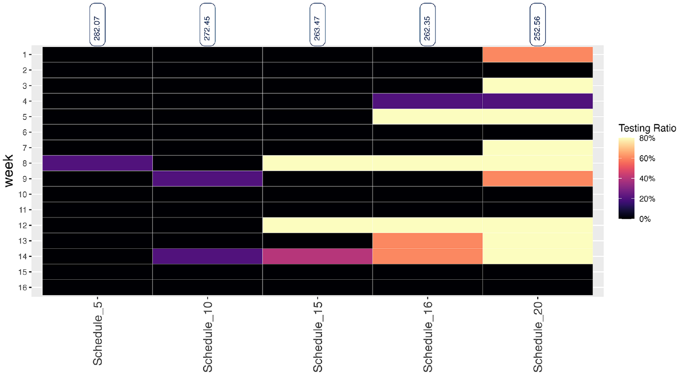
The 5 optimal test schedules with 3 wk of masks. The heatmap shows the subset of the Pareto solutions when 3 wk of masks are used.

Figure 7

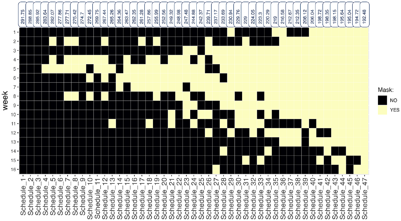
The universal masking schedules of the 47 Pareto optimal solutions. Each column of squares represents a Pareto solution with the corresponding number of end-of-semester infections shown on the top. The color of the 16 squares in each column represents whether universal masking is implemented in those weeks. Black square means no masks are used in that week.

Optimal Solutions: Rapid Antigen Tests

We performed similar analysis with rapid antigen tests for screening. We modified the simulation to reflect the change, which allows individuals to receive test results the same day and transfer to isolation immediately if needed.

By comparing Figures 2 and 8, we see the overall range of the end-of-semester infections was similar between PCR tests and rapid antigen tests. In addition, the effect of tests and masks on end-of-semester infections was consistent between the 2 types of tests. For instance, the highest gray points in Figures 2 and 8 suggested that 584 PCR tests were able to reduce the end-of-semester infections to 292, whereas 8 fewer tests of the rapid antigen type resulted in 1 more infection by the end of the semester. Additional results for the rapid antigen test are shown in Appendix Section E.

Figure 8

The 48 optimal values of the objective in the Pareto front using rapid antigen tests.

Discussion

In this study, we designed and solved a multiobjective simulation optimization problem using NSGA-II. The problem was used to help K-12 schools plan their random screening test and universal masking schedules.

There are some limitations to the study. Certain assumptions were made, such as the number of exposed individuals. This number is uncertain and may differ between schools. In addition, as the virus evolves, some of the parameters we referenced from previous studies—such as the effectiveness of masks, the proportion of asymptomatic infections, and the sensitivity and specificity of PCR and rapid antigen tests—may change. To address these uncertainties, we conducted a sensitivity analysis focusing on 3 key parameters: 1) the effectiveness of masks, 2) the proportion of asymptomatic infections, and 3) the number of exposed individuals on the first day of the semester. The results are provided in Appendix Section F. From the sensitivity analysis, we observed that a higher effectiveness of masks and a greater proportion of asymptomatic infections corresponds to lower end-of-semester infections. In addition, the marginal benefit of 1 additional week of masking is much larger with higher mask effectiveness. While certain parameter values may change as conditions evolve, the method we developed can be easily executed for changes to any parameters and can be tailored to any school.

By solving the 3-objective optimization problem, we successfully verified the negative relationship between the cumulative number of infections and the number of weeks masks are used as well as the negative relationship between the cumulative number of infections and the number of random screening tests, regardless of which type of test we chose. We found that screening tests and masks can be surrogates for each other when prioritizing the value of infections. Thus, if schools prefer one intervention over another, by choosing the aspects they are most concerned about, they can find an optimal policy schedule to implement based on the simulation results. For instance, if schools have a limited supply of tests to distribute during the semester, the Pareto front results can show the lowest number of cumulative infections they can achieve at different levels of mask usage.

Together with masks, we saw that the effect of reducing the end-of-semester infections can be quite similar between rapid antigen and PCR tests. Future work can be done around the cost-effectiveness of the 2 types of tests, as PCR tests are more expensive. In the current framework, we designed AT testing to resemble the schools’ mitigation strategy of screening testing following school-based outbreaks; similarly, masking mandates can be designed to be triggered by the number of infections. Infection-triggered masking would be driven by the disease and not controlled by decision makers directly. Thus, the decision maker could decide the preplanned mask weeks, but the total number of mask weeks would depend on the spread of the disease. This is a possible extension to the model.

Overall, the analysis in this study can offer valuable insights for policy makers in K-12 schools. The conclusions derived from this research can serve as a foundation for making informative decisions regarding random screening tests and universal masking policies. The policies resulting from this model are the most efficient in the sense that they provide the minimum combination of testing and masking to achieve desired infection reduction targets. They also provide the best implementation schedules when the decision maker wants to limit either testing, masking, or both. This benefits students, teachers, and parents by creating a safe learning environment during the pandemic that avoids school closures. In addition, our simulation optimization approach can be generalized to other diseases and be used to make other resource allocation or preventive policy decisions.

Supplemental Material

sj-docx-1-mpp-10.1177_23814683241312225 – Supplemental material for Optimizing Masks and Random Screening Test Usage within K-12 Schools

Supplemental material, sj-docx-1-mpp-10.1177_23814683241312225 for Optimizing Masks and Random Screening Test Usage within K-12 Schools by Yiwei Zhang, Maria E. Mayorga, Julie S. Ivy and Julie L. Swann in MDM Policy & Practice

Footnotes

The authors declared no potential conflicts of interest with respect to the research, authorship, and/or publication of this article. The authors disclosed receipt of the following financial support for the research, authorship, and/or publication of this article: Financial support for this study was provided in part by a grant from UL1TR002489 from the NCATS/NIH and Cooperative Agreement NU38OT000297 from the CSTE and the CDC. The research also received partial support from NC State University. The funding agreement ensured the authors’ independence in designing the study, interpreting the data, writing, and publishing the report.

Ethical Considerations

Not applicable: The study did not use any animal or human subjects. It is a modeling study using with parameters informed by previously published literature.

Consent to participate

Not applicable: The study did not use any animal or human subjects. It is a modeling study using with parameters informed by previously published literature.

Consent for publication

Not applicable.

ORCID iDs

Maria E. Mayorga

Julie L. Swann

Data Availability

The full list of parameters is provided in the appendix. The model R code is shared in a GitHub repository ().

References

World Health Organization. WHO coronavirus (COVID-19) dashboard | WHO coronavirus (COVID-19) dashboard with vaccination data. 2023. Available from: https://covid19.who.int/

Centers for Disease Control and Prevention. COVID-NET interactive dashboard | CDC. 2023. Available from: https://www.cdc.gov/coronavirus/2019-ncov/covidnetdashboard/de/powerbi/dashboard

Abul

Leeder

Gravenstein

. Epidemiology and clinical presentation of COVID-19 in older adults. Infect Dis Clin North Am. 2023;37(1):1–26. DOI: 10.1016/J.IDC.2022.11.001

Ashcroft

Lehtinen

Angst

Low

Bonhoeffer

. Quantifying the impact of quarantine duration on COVID-19 transmission. ELife. 2021;10:1–33. DOI: 10.7554/ELIFE.63704

Monod

Blenkinsop

, et al. Age groups that sustain resurging COVID-19 epidemics in the United States. Science. 2021;371(6536):eabe8372. DOI: 10.1126/science.abe8372

Rosenstrom

Mele

Ivy

, et al. Vaccinating children against COVID-19 is crucial to protect schools and communities. PNAS Nexus. 2022;1(3):pgac081. DOI: 10.1093/PNASNEXUS/PGAC081

Zhang

Mayorga

Ivy

Hassmiller Lich

Swann

. Modeling the impact of nonpharmaceutical interventions on COVID-19 transmission in K-12 schools. MDM Policy Pract. 2022;7(2):23814683221140866. DOI: 10.1177/23814683221140866

UNICEF. COVID:19 Scale of education loss ‘nearly insurmountable’, warns UNICEF. January 2022. Available from: https://www.unicef.org/press-releases/covid19-scale-education-loss-nearly-insurmountable-warns-unicef

Kuhfeld

Soland

Lewis

. Test score patterns across three COVID-19-impacted school years. Educ Res. 2022;51(7):500–6. DOI: 10.3102/0013189X221109178

10.

Duckworth

Kautz

Defnet

, et al. Students attending school remotely suffer socially, emotionally, and academically. Educ Res. 2021;50(7):479–82. DOI: 10.3102/0013189X211031551

11.

Selçuk

Demir

AÇ

Erbay

Özcan

ÖÖ

Gürer

Dönmez

. Anxiety, depression and post-traumatic stress disorder symptoms in adolescents during the COVID-19 outbreak and associated factors. Int J Clin Pract. 2021;75(11):e14880. DOI: 10.1111/IJCP.14880

12.

Leeb

Bitsko

Radhakrishnan

Martinez

Njai

Holland

. Mental health–related emergency department visits among children aged 18 years during the COVID-19 pandemic—United States, January 1–October 17, 2020. MMWR Morb Mortal Wkly Rep. 2020;69(45):1675–80. DOI: 10.15585/MMWR.MM6945A3

13.

Gamez

Carmona

Gamez

Santos

. Evidence of high compliance and fatigue in mask adherence in two mandates in Barcelona, Spain: a naturalistic observational study. Public Health. 2023;225:63–5. DOI: 10.1016/J.PUHE.2023.09.021

14.

The National Center for DEI. State-by-state school mask mandates. 2022. Available from: https://thinkequitable.com/state-by-state-school-mask-mandates/

15.

Kekatos

. Some school districts bring back mask mandates to stem spread of COVID, flu and RSV. ABC News. December 2022. Available from: https://abcnews.go.com/Health/school-districts-bring-back-mask-mandates-stem-spread/story?id=95975555

16.

North Carolina Department of Health and Human Services. StrongSchoolsNC K-12 COVID-19 testing program. NC COVID-19. 2022. Available from: https://covid19.ncdhhs.gov/SchoolTesting#Willentiredistrictsopt-infortheprogramorwillitbeindividualschoolsinadistrict-9274

17.

Montgomery County Public Schools. Spring 2023 reopening guide. February 1, 2023. https://www.montgomeryschoolsmd.org/siteassets/district/reopening2022/languages-2023/msdeguide-011723.pdf

18.

Özüdoğru

Bahçe

Acer

. SARS CoV-2 reinfection rate is higher in the Omicron variant than in the Alpha and Delta variants. Ir J Med Sci. 2022;192:751–6. DOI: 10.1007/S11845-022-03060-4

19.

Nordström

Ballin

Nordström

. Risk of infection, hospitalisation, and death up to 9 months after a second dose of COVID-19 vaccine: a retrospective, total population cohort study in Sweden. Lancet. 2022;399(10327):814–23. DOI: 10.1016/S0140-6736(22)00089-7

20.

Chernozhukov

Kasahara

Schrimpf

. The association of opening K–12 schools with the spread of COVID-19 in the United States: county-level panel data analysis. Proc Natl Acad Sci U S A 2021;118(42):e2103420118. DOI: 10.1073/pnas.2103420118

21.

Rosenstrom

Ivy

Mayorga

, et al. High-quality masks reduce COVID-19 infections and deaths in the US. MedRxiv. Epub ahead of print January 28, 2021. DOI: 10.1101/2020.09.27.20199737

22.

Dinnes

Sharma

Berhane

, et al. Rapid, point-of-care antigen tests for diagnosis of SARS-CoV-2 infection. Cochrane Database Syst Rev. 2022(7):CD013705. DOI: 10.1002/14651858.CD013705.PUB3/

23.

Kortela

Kirjavainen

Ahava

, et al. Real-life clinical sensitivity of SARS-CoV-2 RT-PCR test in symptomatic patients. PLoS One. 2021;16(5):e0251661. DOI: 10.1371/JOURNAL.PONE.0251661

24.

Lin

Carlquist

Sinclair

Hall

Lopansri

Bennett

. Experience with false-positive test results on the taqpath real-time reverse transcription-polymerase chain reaction coronavirus disease 2019 (COVID-19) testing platform. Arch Pathol Lab Med. 2021;145(3):259–61. DOI: 10.5858/ARPA.2020-0612-LE

25.

Ching-Shih (Vince) Tsou. nsga2R: elitist non-dominated sorting genetic algorithm. 2022. Available from: https://cran.r-project.org/web/packages/nsga2R/index.html

26.

R Core Team. R: The R project for statistical computing. 2023. Available from: https://www.r-project.org/

27.

Zhang

Mayorga

Ivy

Swann

. Multi-criteria simulation optimization for COVID-19 testing in schools. Proceedings of the Winter Simulation Conference; San Antonio, TX; December 10–13, 2023; pp 1006–17.

Supplementary Material

Please find the following supplemental material available below.

For Open Access articles published under a Creative Commons License, all supplemental material carries the same license as the article it is associated with.

For non-Open Access articles published, all supplemental material carries a non-exclusive license, and permission requests for re-use of supplemental material or any part of supplemental material shall be sent directly to the copyright owner as specified in the copyright notice associated with the article.

0.00 MB

1.42 MB