Sage Journals: Discover world-class research

Abstract

The authors use Current Population Survey 2016 to 2021 quarterly data to analyze changes in household joblessness across metropolitan areas in the United States during the coronavirus disease 2019 pandemic. The authors first use shift-share analysis to decompose the change in household joblessness into changes in individual joblessness, household compositions, and polarization. The focus is on polarization, which is the result of the unequal distribution of individual joblessness across households. The authors find that the rise in household joblessness during the pandemic varies strongly across U.S. metropolitan areas. The initial stark increase and subsequent recovery are due largely to changes in individual joblessness. Polarization contributes notably to household joblessness but to varying degree. Second, the authors use metropolitan area–level fixed-effects regressions to test whether the educational profile of the population is a helpful predictor of changes in household joblessness and polarization. They measure three distinct features: educational levels, educational heterogeneity, and educational homogamy. Although much of the variance remains unexplained, household joblessness increased less in areas with higher educational levels. The authors show that how polarization contributes to household joblessness is shaped by educational heterogeneity and educational homogamy.

Keywords

household joblessness COVID-19 polarization educational profiles metropolitan areas

In this study we analyze how household joblessness developed across metropolitan areas during the coronavirus disease 2019 (COVID-19) pandemic in the United States. There is long-standing interest in sociology in the spatial concentration of economic disadvantages in the United States. Many scholars have documented that poverty has become more spatially concentrated in metropolitan areas since the 1970s (e.g., Iceland and Hernandez 2017; Jargowsky 1996; Kneebone, Nadeau, and Berube 2011; Krivo et al. 1998; Massey and Eggers 1990, 1993; Quillian 2012). Wilson’s (1987, 1997) seminal work identified the spatial concentration of joblessness, particularly among men in African American neighborhoods, as critical to understanding urban poverty and its far-reaching consequences (for quantitative confirmation of this concentration, see, e.g., Quillian 2003; Wagmiller 2007).

This study shifts the focus from male joblessness to the spatial concentration of joblessness of entire households. The link between labor market outcomes and families and households has been widely studied in sociology. For instance, research has paid particular attention to Wilson’s (1987, 1997) prediction that one of the far-reaching consequences of the spatial concentration of male joblessness in U.S. metropolitan areas is the disruption of family formation processes (e.g., Fossett and Kiecolt 1993; Massey and Shibuya 1995; Sampson 1987; South and Crowder 1999, 2010; South and Lloyd 1992). Another strand of literature highlights educational matching as a main reason for the accumulation of economic disadvantages in households (e.g., Blossfeld and Buchholz 2009; Breen and Salazar 2011; Eika, Mogstad, and Zafar 2019; Schwartz 2010; Ultee, Dessens, and Jansen 1988). Despite the vast attention paid by sociologists to the link between family formation processes in local marriage markets and spatial concentration of joblessness, there is surprisingly little research on how these two dimensions of the accumulation of disadvantage combine (i.e., the spatial concentration of accumulated joblessness in households).

Household joblessness is the phenomenon when no working-age household member is in employment. Existing research shows that household joblessness has detrimental outcomes for all household members including children. The likelihood of poverty and material deprivation is particularly high when entire households become jobless because one or more members lose their jobs (de Graaf-Zijl and Nolan 2011; Scutella and Wooden 2004; see also our discussion in our concluding section). Furthermore, the experience of living in a household in which no parent is working detrimentally affects children’s education and labor market outcomes over and above the impact of poverty (Curry, Mooi-Reci, and Wooden 2019, 2022; Ermisch, Francesconi, and Pevalin 2004; Mooi-Reci, Wooden, and Curry 2020). Thus, household joblessness has immediate adverse effects on household members, and it entrenches social inequalities in the long term. Our first contribution is to analyze whether the COVID-19 economic crisis has exacerbated household joblessness across U.S. metropolitan areas.

Our second contribution is to assess whether the development of household joblessness across U.S. metropolitan areas during the pandemic results from an accumulation of disadvantages in some households. One reason for the dearth of research on household joblessness might be the assumption that individual joblessness and household joblessness move in lockstep. However, previous work shows a decoupling between rising individual employment rates and stagnant or increasing rates of household joblessness in many advanced economies over the past several decades (Corluy and Vandenbroucke 2017; Gregg, Scutella, and Wadsworth 2008). Gregg et al. (2008) and Gregg and Wadsworth (2001) called this process polarization, defined as the deviation in household joblessness from a counterfactual that emerges if joblessness is randomly distributed across households. Polarization emerges because households accumulate employment risks, most visible in the rise of dual-earner households on one side and completely jobless households on the other. Polarization implies that assessing individual labor market outcomes cannot accurately capture developments in household joblessness and thus misses an essential dimension of social inequality. Our particular interest is in how this accumulation of disadvantages in households is spatially concentrated in some metropolitan areas.

As our third contribution, we propose that focusing on the educational profile of the population provides a starting point to explaining the stark differences in household joblessness and polarization across metropolitan areas. Drawing on sociological studies of the wider geographical distribution of income segregation, income inequality, skill-based wage premia, and mobility across the United States, we argue that inequality in economic outcomes such as in the likelihood of job loss in a labor market is an outcome of its human capital profile as reflected in the population’s educational levels and educational heterogeneity (Moller, Alderson, and Nielsen 2009; Nielsen and Alderson 1997; VanHeuvelen and Copas 2019). How this translates into household joblessness depends on how education is clustered in households, which can be traced to dynamics of household formation, especially educational homogamy (Greenwood et al. 2014; Raymo and Xie 2000; Schwartz and Mare 2005). Education is thus a key link between individual risks for joblessness and their accumulation in households. The educational stratification in household and labor market formation (e.g., in the shape of greater homogamy at different levels of education and educational heterogeneity) means that labor markets with different educational profiles shape household joblessness and polarization risks.

Our analysis uses quarterly data from the Current Population Survey (CPS) for 2016 to 2021 (Flood et al. 2021). Quarterly data allow us to follow the developments of the pandemic closely. Like previous work on the spatial concentration of economic disadvantage we focus on metropolitan areas in the United States (e.g., Jargowsky 1996; Massey and Eggers 1990, 1993; Reardon and Bischoff 2011; Wagmiller 2007). The analysis proceeds in two steps. First, we use shift-share analysis to decompose changes in household joblessness since the onset of the pandemic (Biegert and Ebbinghaus 2022; Gregg et al. 2008; Gregg and Wadsworth 2001). Beyond describing metropolitan area trends in household joblessness, the decomposition enables us to assess how much of the change in household joblessness can be attributed to polarization, i.e., the unequal distribution of joblessness across households. Second, we use panel fixed-effects models at the level of metropolitan areas to assess whether educational profiles of labor markets ameliorated or exacerbated the increase in household joblessness and the contribution from polarization during the pandemic. Before discussing details of our data and analysis, presenting results, and concluding, we provide the theoretical framework and contextual information on the COVID-19 pandemic.

Background

Polarization in Household Joblessness Because of Accumulation and Absorption

When people lose their jobs in economic downturns, an increase in households in which no one is working is almost unavoidable. But the extent to which individual job loss translates to household joblessness depends on how job loss is distributed. We use a framework proposed by Gregg et al. (2008) and Gregg and Wadsworth (2001) that describes the unequal distribution of individual joblessness across households as polarization. Importantly, the benchmark against which we measure polarization is a random distribution of joblessness across households. The accumulation scenario comes into play when job loss disproportionately affects households that are more likely to be thrown into household joblessness. This could be the case if many single earner households are hit or if job loss is so concentrated that both earners in dual-earner households lose their job. These households would thus accumulate joblessness while other dual-earner households remain unscathed and keep both jobs. In Gregg et al.’s (2008) and Gregg and Wadsworth’s (2001) framework, accumulation of individual joblessness in households means positive polarization (Biegert and Ebbinghaus 2022). By contrast, in the absorption scenario job loss is concentrated so that households with only one earner keep their jobs and dual-earner households lose one job but keep one household member in employment. Households would thus absorb the job loss of single members, leading to negative polarization. In the accumulation scenario, there is a greater increase in household joblessness compared with a random distribution of job loss. In the absorption scenario, there is less.

The few existing explanations of why some labor markets foster household joblessness and accumulation, whereas others show absorption have received only mixed empirical support. Previous research applying the polarization framework describes national trends since the 1970s and changes during the 2008 economic crisis (Biegert and Ebbinghaus 2022; Corluy and Vandenbroucke 2017; Gregg et al. 2008; Gregg and Wadsworth 2001). To explain variation in household joblessness and polarization across economies, these studies invoke typical household structures and welfare regimes. By and large, there is evidence that countries with more traditional household structures in which single breadwinners work in protected insider jobs are more negatively polarized. By contrast, countries with individualized family structures and liberal or universal welfare support show more positive polarization (Gregg et al. 2008; Gregg and Wadsworth 2001). However, there are exceptions. For instance, given its residual welfare state and prevalence of nontraditional household structures, the United States showed surprisingly low levels of polarization in the decades leading up to the 2008 economic and financial crisis (Gregg et al. 2008). Moreover, the observed secular trends do not hold in times of economic crisis. During the 2008 economic and financial crisis and thereafter, traditional male breadwinner countries in the European South showed especially large increases in polarization (Biegert and Ebbinghaus 2022; Corluy and Vandenbroucke 2017). From a sociological perspective, there is of course a wealth of research to draw on when interested in why households and labor markets might differ in their proclivity to accumulate employment risks. Arguing from a micro perspective of employment risks and their clustering in households, in the following section we propose that educational profiles of labor markets can help explain household joblessness and polarization.

Educational Profiles of Labor Markets

Why does the share of jobless households vary across local labor markets? Why does household joblessness increase more strongly in some local labor markets during an economic downturn? The sociological literature highlights racial and educational differences underlying the spatial concentration of economic disadvantages. Most prominently, Wilson’s (1987, 1997) seminal work has inspired a wealth of research on how racial divisions underlie agglomerations of economic disadvantage, such as joblessness and poverty (e.g., Jargowsky 1996; Massey and Eggers 1990, 1993; Quillian 2003; Reardon and Bischoff 2011; Wagmiller 2007). Linking the spatial concentration of individual disadvantages to the concentration of disadvantages in households, the literature detects structural differences in how these racial disparities in economic outcomes connect to family formation processes. For instance, a decline in marriageable men in an area because of increased joblessness is associated with decreased marriage rates (e.g., Massey and Shibuya 1995), increased nonstandard family structures (e.g., Fossett and Kiecolt 1993), and teenage and nonmarital fertility (e.g., South and Crowder 1999, 2010; South and Lloyd 1992). Another strand of literature highlights the important connections between education and skills, sectoral transformations, and geographic location. Since the 1970s, sectoral and spatial shifts in the leading industries in U.S. metropolitan areas, as well as spatial restructuring of work, and labor markets (i.e., “spatialization” of employment), have increased the importance of geography and led to concentration of high-skill and low-skill jobs in large urban areas (Glaeser and Saiz 2004; Mulligan, Reid, and Moore 2014; Sassen 1990; Wallace and Brady 2001; Wilson 1997). The educational makeup of geographical areas has been shown to be strongly associated with income inequality (Moller et al. 2009; Nielsen and Alderson 1997; VanHeuvelen and Copas 2019). Building on these arguments, we focus on education as the central variable to explain geographical concentration of individual disadvantages and how they accumulate in households. We argue that how economic crises affect different local labor markets largely depends on their sectoral and occupational structures. To explain how shocks affect spatial inequality, we thus need to consider the distribution of jobs with different degrees of vulnerability across local labor markets. We furthermore need to understand how jobs of varying risk are clustered within households. We propose that the educational profile of the population in a local labor market provides a parsimonious way of combining considerations about labor market structures and household compositions. Our argument relies primarily on individuals, their education, and how they cluster in households. But because the educational composition of a labor market’s population yields externalities, we need to look at the aggregate educational profile of a local labor market to fully understand variation in household joblessness and polarization between them. We focus on three aspects of the education profile of the population in a metropolitan area: educational level, educational heterogeneity, and educational homogamy.

It is well established that workers with higher educational attainment experience fewer job losses during economic downturns, whereas lower education increases the likelihood of job loss (Farber 2005, 2015; Kesler and Bash 2021). For instance, Farber (2015) found that although there is a cyclical pattern in job loss for all educational groups in the United States between 1981 and 2013, job loss rates are dramatically higher for less educated workers. Kesler and Bash (2021) found that having low educational attainment at least doubled the risk for job loss during the COVID-19 crisis. Furthermore, more educated workers find new employment more quickly after job loss, shortening unemployment spells (Farber 2015; Gesthuizen, Solga, and Künster 2011; Klein 2015; Riddell and Song 2011). Educational levels are thus important to understand varying levels of job loss during economic downturns across labor markets. Overall educational levels are also essential for how joblessness is distributed across the labor market and households. For instance, lower educated individuals profit from living in areas with higher educational levels. Areas with high stocks of human capital deal better with economic shocks and yield positive externalities for their lower educated occupants (Glaeser and Saiz 2004). Winters (2013), for instance, found that human capital externalities significantly decrease their probability to become unemployed. By extension of individual joblessness, we thus expect household joblessness to rise more strongly in labor markets with lower levels of education.

Beyond educational levels, the relative position of individuals in the educational distribution of a labor market will affect their chances to lose their job in an economic downturn. The distribution of human capital among the population is the main determinant of inequality in a labor market (Mincer 1970). Studies of U.S. labor markets show that educational heterogeneity is one of the central drivers of within labor market inequality in economic outcomes (Moller et al. 2009; Nielsen and Alderson 1997; VanHeuvelen and Copas 2019). During an economic downturn, greater educational inequality might lead to a concentration of job loss among the lower educated. Educational heterogeneity thus should affect the inequality in the likelihood of individual job loss. This might be reflected in polarization of household joblessness as well to the degree that households accumulate individual job loss risks.

How much educational levels and heterogeneity affect household joblessness and polarization depends on how education is clustered in households. Educational clustering in households is driven by assortative mating. Highly educated couples are more likely to be dual earners in secure jobs, lower educated households are more likely to be in precarious employment or jobless (Blossfeld and Buchholz 2009; Breen and Salazar 2011; Schwartz 2010; Ultee et al. 1988). Educational homogamy thus increases the likelihood of positive polarization. The United States has comparatively high levels of educational homogamy (Greenwood et al. 2014; Schwartz and Mare 2005). But labor markets differ in how much they attract homogamous households. So-called superstar cities and large metropolitan areas, for instance, house significant shares of highly educated power couples because they offer them rewarding job opportunities (Costa and Kahn 2000).

We derive some guiding expectations: first, higher educational levels should prohibit stark increases in household joblessness. Second, whether household joblessness is exacerbated by positive polarization depends on how unequally education is distributed and how it is clustered in households. When low educational levels are combined with greater educational heterogeneity and high homogamy, we can expect higher household joblessness because of higher individual joblessness but also because higher polarization leads to disproportionate household joblessness at a given level of individual joblessness because households accumulate risks. By contrast, an economic downturn should increase household joblessness less in labor markets that combine high educational levels and low heterogeneity with lower levels of homogamy. That is because of lower numbers of jobs lost but also because these labor markets should have lower polarization, and they might even show negative polarization (i.e., absorption).

Context: The COVID-19 Economic Crisis in U.S. Metropolitan Areas

We assess the development of household joblessness during economic downturns, the role of polarization, and the explanatory power of educational profiles of local labor markets by analyzing the COVID-19 pandemic in U.S. metropolitan areas. The COVID-19 pandemic caused job loss in the United States on a scale not seen since the 2008 Great Recession. The existing evidence also shows large spatial variation in the employment impacts across U.S. labor markets (Dalton 2020; Mulligan 2023).

Several specificities of the COVID-19 crisis compared with other economic downturns are worth noting. First, job loss during the pandemic was concentrated around particular subgroups of the population. For instance, an unfavorable distribution in occupations widened the white-nonwhite (Couch, Fairlie, and Xu 2020; Dias 2021) and gender (Alon et al. 2020; Collins et al. 2021) gaps in unemployment. In terms of occupations, areas with large hospitality sectors saw the steepest initial increases in unemployment, whereas areas with higher shares in finance and insurance were less affected (Dalton 2020). The COVID-19 crisis also incited the so-called great resignation: the massive number of workers who voluntarily left their jobs. In 2021, monthly resignation rates across all industries in the United States were the highest in the past 20 years, while job openings were higher than the number of hires (Faccini, Melosi, and Miles 2022). How job loss was concentrated across occupations and where it was located geographically might therefore differ from other economic downturns.

Second, the U.S. welfare state traditionally compensates for the loss of earnings with only meager unemployment benefits. Household joblessness is therefore a particularly problematic situation. Yet the U.S. government amended payments during the initial phase of the pandemic via the Coronavirus Aid, Relief, and Economic Security Act. Still, the termination of the emergency unemployment compensation puts a significant share of the population at risk for poverty. Third, lockdown and isolation rules might have affected how households reacted to job loss compared with previous economic downturns. For instance, there is mixed evidence that households “doubled up” during previous crises to cope with income loss and, especially during the Great Recession, to cope with housing debt with the collapse of the housing market (Bitler and Hoynes 2015; Wiemers 2014). Although changes in household composition during previous crises such as the Great Recession were more persistent, during the COVID-19 pandemic, there is evidence that headship rates decreased early in the pandemic but returned to prepandemic levels within few months (García and Paciorek 2022).

We analyze metropolitan areas as local labor markets. Recent literature on U.S. local labor markets prefers looking at commuting zones (e.g., Autor and Dorn 2013; VanHeuvelen and Copas 2019). Commuting zones more clearly outline local labor markets as they are constituted to represent the geographic area that clusters individuals’ work travels. For analyzing variation across local labor markets an added advantage of commuting zones is their greater case number (>700). However, no data set that allows for the creation of commuting zones offers timely data on the COVID-19 pandemic. There are several good reasons for analyzing metropolitan areas. First, because more than 80 percent of Americans live in metropolitan areas, their analysis provides an important insight into a large proportion of the U.S. population (U.S. Census Bureau 2022). There is a rich literature on spatial economic inequality in the United States that we can connect to. Metropolitan areas in the United States serve as key spatial units to study joblessness, economic segregation, poverty, and income inequality (e.g., Iceland and Hernandez 2017; Jargowsky 1996; Kneebone et al. 2011; Krivo et al. 1998; Massey and Eggers 1990, 1993; Quillian 2003, 2012; Reardon and Bischoff 2011). This is because, second, metropolitan areas are a good approximation of local labor markets as they are made up of a large population center with dense economic activity, and adjacent communities that economically and socially interact with the center (Fowler and Jensen 2020). However, variations between metropolitan labor markets lead to significant inequalities between U.S. cities (Mulligan et al. 2014). Part of the explanation for variation between metropolitan areas is that third, they have different educational profiles. A higher demand and “premium” pay in some metropolitan areas lead to the concentration of skills (Li, Wallace, and Hyde 2019; Liu and Grusky 2013). Essletzbichler (2015) found that metropolitan areas with large shares of the top 1 percent are characterized by higher levels of skill polarization, higher labor force participation and lower unemployment for those with little formal education. Metropolitan areas also vary in their attractiveness to different household compositions (e.g., homogamous power couples) (Costa and Kahn 2000). Processes of household formation are strongly concentrated within metropolitan areas (Liao and Özcan 2013). Finally, the COVID-19 pandemic’s impact was strongest in metropolitan areas. The higher early infection rates of COVID-19 in more densely populated urban areas caused severe employment losses early on. Compared with rural residents, urban adults were more often unpaid for missed hours, inability to work or to look for work (Brooks, Mueller, and Thiede 2021). These losses could have longer term effects on persistent job reductions in metropolitan areas (Cho, Lee, and Winters 2021).

CPS 2016 to 2021¹

Data and Sample

We use repeated monthly cross-sectional data (pooled in quarters) from the CPS 2016 to 2021 as provided by IPUMS (Flood et al. 2021). Our analysis proceeds in two steps. First, we conduct a shift-share decomposition of the change in household joblessness across metropolitan areas from before the pandemic to since its onset (Gregg et al. 2008; Gregg and Wadsworth 2001). The decomposition enables us to separate the contribution of polarization to changes in household joblessness from the contributions of changes in individual joblessness and changes in household size. Second, we use our measures of overall changes in household joblessness and the contribution of polarization at the metropolitan area level as derived from the decompositions as dependent variables. We use panel fixed-effects regressions to investigate their variation between metropolitan areas with different educational profiles during the pandemic.

Monthly CPS data offer large sample sizes of about 125,000 individuals in 50,000 households and a rich set of variables describing employment, sociodemographics, and family-structure status of these households. Sample sizes vary widely for metropolitan areas. Some areas have fewer than 10 observations in some months, whereas others consistently have many thousands. To achieve robust estimates, we pool data in quarters. Our data includes 24 quarters starting with Q1 2016 and ending in Q4 2021. We include all households with at least one working-age member (16–64 years). Both the shift-share analysis and the panel fixed effects analyses operate at the (aggregate) level of metropolitan areas. To ensure that we estimate all our metropolitan area–level indicators robustly, we exclude metropolitan areas with less than 50 households in any quarter. That leaves us with 204 of the original 261 metropolitan areas. Aggregate-level variables are constructed on the basis of, on average, 786 working-age individuals in 409 households per quarter and metropolitan area. We use survey weights included in CPS throughout to calculate aggregate level indicators. Our metropolitan area–level data set contains 4,896 cases (204 metropolitan areas over 24 quarters). Our multivariate models use the information from before the pandemic only as the benchmark for which to calculate changes, so the effective sample is reduced to 1,428 (204 metropolitan areas over 7 quarters).

Variables

Our two main outcomes of interest are household joblessness and polarization of household joblessness. To construct our measure of household joblessness, we consider every individual as employed (0) who indicates being employed at time of interview. We also code them as employed when they are in the armed forces or when they were not at work last week but indicate that they have a job. We use this inclusive coding as not to overestimate joblessness. We code as jobless (1) every other employment status: unemployed or not in the labor force, including housework, education, inability to work, early retirement, and unpaid work. We then code every household as jobless (1) if no working-age member is employed. Every household with at least one member in employment is assigned not jobless (0). Thus, our conception of a household is based on residency rather than family relations. As our underlying interest is in the pooling of resources in households, our measures will thus be conservative estimates of deprivation because some households who are not composed of families might not pool. We calculate the household joblessness rate at the level of metropolitan areas as the rate of working-age individuals who live in entirely jobless households.

Our measure of polarization captures the inequality in the distribution of joblessness across households. We follow Gregg and Wadsworth (2001), who measured polarization as the difference between the actual rate of household joblessness and a counterfactual household jobless rate. The counterfactual household joblessness rate is what would emerge if the distribution of joblessness across individuals were random, i.e., every individual had the same probability of being jobless, with

\begin{matrix} {\hat{w}}_{k} = n^{k} \end{matrix},

(1)

where ${\hat{w}}_{k}$ is the counterfactual household joblessness rate for a household of $k$ working-age household members and $n$ is the individual joblessness rate in a metropolitan area. This counterfactual household joblessness rate does not entail any inequality in the likelihood of different households being jobless. It can be calculated using the individual joblessness rate of a metropolitan area and information about household sizes as defined by the number of working-age members. A household with only one working-age member has the same counterfactual rate as the overall individual joblessness rate in a given metropolitan area at a given time. The counterfactual household joblessness rate gets lower for households with more working-age members. It is calculated as the individual joblessness rate to the power of n, with n being the number of working-age household members. On the aggregate level of metropolitan areas, the counterfactual household joblessness rate is then given by the individual joblessness rate weighted by the distribution of working-age individuals across households of different sizes with

\begin{matrix} \hat{w} = \sum_{k = 1}^{K} S_{k} {\hat{w}}_{k} = \sum_{k = 1}^{K} S_{k} n^{k} \end{matrix},

(2)

where $S_{k}$ is a weight that indicates the proportion of the population living in households of size $k$ . A metropolitan area with a disproportional number of single households, for instance, would have a relatively higher counterfactual household joblessness rate at a given individual joblessness rate.

Polarization is the difference between this counterfactual and the actual rate of household joblessness (i.e., the proportion of working-age individuals living in households without any employment):

\begin{matrix} P = w - \hat{w} = \sum_{k = 1}^{K} S_{k} w_{k} - \sum_{k = 1}^{K} S_{k} {\hat{w}}_{k} = \sum_{k = 1}^{K} S_{k} (w_{k} - n^{k}) \end{matrix} .

(3)

If joblessness is distributed randomly, the counterfactual and actual household joblessness rates become identical; thus, polarization becomes 0 (neutral). Negative polarization indicates that work is distributed so that fewer households are without work than predicted by random distribution. We could imagine this to be the case in contexts with strong male breadwinner models where the typical family model entails one earner with several dependents. Polarization turns positive when there are more jobless households than expected. We could imagine this in contexts with many multiple-earner households on the one side and many households with no one working on the other. Positive polarization conforms to our understanding of risk accumulation in precarious jobless households that contrast with others that are more fortunate.

The information on individual and household joblessness, polarization, and household sizes are all we need for the shift-share analysis. For our metropolitan area–level panel analysis, we create additional measures that capture the makeup of metropolitan area labor markets and their demographic composition.

We base the measures for our educational profiles on years of schooling of all 25- to 64-year-old individuals (as transformed from detailed information on educational attainment following Jaeger 1997). We measure educational levels as the average number of years of schooling in a metropolitan area–quarter. Our measure of educational heterogeneity is a Theil index of years of schooling. The index provides a measure of educational dividedness that takes a high value when individuals have varying numbers of years in education and a low value when most individuals have similar numbers of years in education. Finally, we measure the prevalence of educational homogamy as the correlation between the higher educated partner and the lower (or equally) educated partner in partner households (married and cohabiting). Partnership status is defined in reference to the household head in the CPS.

To be able to separate the predictive power of educational profiles for our dependent variables, we include a host of other sociodemographic measures and indicators for labor market structures, which we construct as shares at the metropolitan area level. Our choices follow literature on spatial income inequality in the United States (Moller et al. 2009; VanHeuvelen and Copas 2019). To measure the ethnic composition of a metropolitan area, we calculate the share of the Black (% Black) and the Hispanic (% Hispanic) population. We measure the share of migrants as percentage of the working-age population (% migrants). We measure the prevalence of older people by calculating the share of individuals 65 years and older of the total population (% older). We measure the prevalence of single households by calculating the share of households without a partner as a percentage of the total number of households (% single). We measure the population size of metropolitan areas as the total population in absolute numbers (population size). Finally, we measure the distribution of the population across the center and periphery of the metropolitan area (% living in the central city).

To measure the economic prosperity of a metropolitan area, we use the median household income (medianinc) equivalized by household size (Organisation for Economic Co-operation and Development equivalence scale). Income data is not available in the monthly CPS data. We calculate annual median household incomes using the CPS Annual Social and Economic Supplement. To model labor market sectoral structures, we calculate four indicators. First, we measure the size of the government sector by the share of workers in public administration (% gov). We measure the size of the manufacturing sector by the share of workers in manufacturing (% manu). Third, we measure the size of the finance, insurance, and real estate (FIRE) sector by the share of workers in finance, insurance, and real estate service jobs (% FIRE). Finally, we measure the size of the service sector as the share of workers in all other service jobs (% service). Table A1 in the Appendix shows mean and standard deviation for all variables in our models.

Analytical Strategy

Shift-Share Decomposition

Shift-share decomposition of changes in household joblessness uses data on individuals in households to assess changes in joblessness at the individual level and the household level (Gregg et al. 2008; Gregg and Wadsworth 2001). The decomposition determines which part of the change in household joblessness can be attributed to changes in individual joblessness, changes in household sizes, and changes in polarization. We want to analyze changes in household joblessness since the onset of the pandemic. We calculate changes in household joblessness and changes in the contributing factors for each quarter starting from Q2 2020. Our comparison is the average of the respectively same quarter for the years 2016 to 2019. By comparing the same quarter, we parse out seasonality effects. Using the three-year average as a benchmark helps us estimate changes that were induced by the pandemic rather than expressing a predetermined trend.

The change in household joblessness can be broken down into the change in the counterfactual household joblessness rate and the change in the actual household joblessness rate subtracting the counterfactual household joblessness rate (equation 4):

\begin{matrix} Δ w = Δ \hat{w} + Δ (w - \hat{w}) \end{matrix} .

(4)

Following from equation 3, the two terms can be calculated using information on the change in the individual joblessness rate $n$ for households of size $k$ weighted by the change in the share $S$ of individuals living in households of size $k$ and information on the change in household joblessness of households of size $k$ (equation 5):

\begin{matrix} Δ w = \sum_{k = 1}^{K} Δ (S_{k} n^{k}) + \sum_{k = 1}^{K} Δ (S_{k} (w_{k} - n^{k})) \end{matrix} .

(5)

Eventually, the decomposition breaks down over-time shifts in household joblessness into fluctuations in individual joblessness, structural changes in household sizes, and polarization (equation 6):

\begin{array}{l} Δ w = \sum_{k = 1}^{K} Δ S_{k} (0.5 n_{t}^{k} + 0.5 n_{t + 1}^{k}) \\ + \begin{matrix} \begin{array}{l} \sum_{k = 1}^{K} Δ n^{k} (0.5 S_{k, t} + 0.5 S_{k, t + 1}) \\ + \sum_{k = 1}^{K} Δ S_{k} (0.5 {(w_{k} - n^{k})}_{t} + 0.5 (w_{k} - n^{k})_{t + 1}) \\ + \sum_{k = 1}^{K} Δ (w_{k} - n^{k}) (0.5 S_{k, t} + 0.5 S_{k, t + 1}) . \end{array} \end{matrix} \end{array}

(6)

First, household joblessness changes because of structural changes in household size (first right-hand sum term in equation 6). Households can pursue different strategies to buffer job loss of individuals. For instance, they might “double up” (i.e., merge households, to pool resources) (Bitler and Hoynes 2015; Wiemers 2014). Unemployment might also cause households to split up (Brand 2015). Such developments on a larger scale would affect a metropolitan area’s household jobless rate. In our decomposition, we can show how much such developments contribute to the overall change in household joblessness.

Second, change in individual employment (second right-hand sum term in equation 6) during the pandemic, will necessarily affect the expected probabilities of household joblessness. More individuals without a job means more households entirely without work when job loss is distributed randomly. In the shift-share analysis, we attribute the observed changes in household joblessness to changes in individual joblessness for each household size (calculated as the change in the individual joblessness rate to the power of the number of working-age members in the respective quarter). When decomposing the change in household joblessness, we thus attribute that part to the fluctuations in individual joblessness that equals the change in counterfactual household joblessness.

The third component contributing to the overall change in household joblessness is the change in polarization. The decomposition breaks down changes in polarization into a between household-type and a within household-type component. Between-polarization (third right-hand sum term equation 6) changes when job loss is unequally allocated across households of different sizes. For instance, between-polarization would rise if more single households lost their jobs and become household jobless, whereas couple households keep their jobs. Within-polarization (fourth right-hand sum term in equation 6) changes when joblessness is unequally distributed among households of the same size. This might result from households’ facing different risks for job loss because of educational differences. In our presentation of the decomposition, we will not focus on the two components of polarization. Instead, we present figures on polarization in total, which we obtain by simply adding the two components up. We conduct the shift-share decomposition for the merged sample of all 204 U.S. metropolitan areas and for all metropolitan areas separately.

Metropolitan Area–Level Panel Fixed-Effects Models

In our multivariate analysis, we estimate how the development of household joblessness and the contribution of polarization to changes in household joblessness differed between metropolitan areas with different educational profiles. Our baseline model specification is as follows:

\begin{matrix} Y_{i t} = c_{i} + β_{Q} Q_{i t} + β_{E} E_{i t} + β_{Q E} Q_{i t} E_{i t} + β_{Z} Z_{i t} + ϑ_{i} + ε_{i t} \end{matrix}

(7)

where $Y_{i t}$ is the change in household joblessness or the contribution of polarization to changes in household joblessness in a metropolitan area $i$ in quarter $t$ compared with the prepandemic benchmark of the respective variable. On the right-hand side, $c_{i}$ is the metropolitan area time-constant intercept. $Q_{i t}$ is an indicator of the quarter. $E_{i t}$ represents our three measures of education (i.e., levels, heterogeneity, and homogamy). $Q_{i t} E_{i t}$ is the interaction term of the quarter and the educational measures. We use these interactions (up to four-way) to estimate differences between the metropolitan areas in the most flexible way and to capture all combinations of education measures, which generate different “education profiles.” $Z_{i t}$ represents our battery of time-varying metropolitan area–level covariates (% Black, % Hispanic, % migrants, population size, % single, % older, median equivalized income, % public sector, % manufacturing, % FIRE, % other services, % living in central city). We include them as one quarter lags, as these variables are plausibly endogenous to our educational variables and/or outcomes. $ϑ_{i}$ and $ε_{i t}$ are the time-constant and the time-varying component of the error term. We use fixed-effects models to eliminate bias from time-constant unobserved heterogeneity between the metropolitan areas (Allison 2009). The fixed-effects transformation eliminates the time-constant error term $ϑ_{i}$ as well as the time-constant intercept. We cluster standard errors at the metropolitan area level.

The fixed-effects model estimates coefficients for the association between deviations from the mean of metropolitan areas’ change in household joblessness or the mean contribution of polarization to changes in household joblessness and the deviations from the mean of the right-hand side variables. We do not report the estimated regression coefficients from these specifications because of the complexity of interpreting them and because our quarter dummies and their two-way, three-way, and up to four-way interactions with our three key education measures generate numerous coefficients (but see Tables A2 and A3 for the full models). Instead, we show and discuss the predicted values from these regressions as profile plots. The profile plots allow us to illustrate changes in household joblessness and the contribution from polarization to these changes for metropolitan areas with select combinations of education measures that describe specific education profiles.

Results

Household Joblessness and Its Decomposition in All U.S. Metropolitan Areas Combined

We first show overall trends in individual and household joblessness and polarization in all U.S. metropolitan areas combined. Figure 1 illustrates the clear rise in joblessness both for individuals and households during the pandemic (left-hand y-axis). Although the rate of household joblessness is naturally lower, an average 10 percent of the working-age population lives in entirely jobless households even before the pandemic hit. With the onset of the crisis, we see an uptick of about 5 percentage points. In 2021, both individual and household joblessness are trending toward prepandemic levels, although household joblessness plateaus slightly. That is because polarization increases too (right-hand y-axis). Polarization hovers around 0.4 percentage points before the pandemic but increases to 0.8 percentage points at its pandemic peak. At this point, therefore, household joblessness is 0.8 percentage points higher than we would expect for a random distribution of individual joblessness across households. Polarization also shows some seasonal variance, with comparatively low levels in Q2 in the years before the pandemic. In subsequent analyses all figures are always compared with the respective quarter before the pandemic, thus seasonality should not bias our findings. Before and since the pandemic, polarization is always positive, which indicates accumulation of employment risks in households.

Figure 1.

Individual and household joblessness rates and polarization in metropolitan area United States, 2016 to 2021.

In our shift-share analysis we use the respective average quarters 2016 to 2019 as the prepandemic baseline. We decompose changes relative to this baseline for each quarter from Q2 2020 until Q4 2021. Figure 2 displays the decomposition for the entire metropolitan area United States (i.e., the population-weighted average of the 204 metropolitan areas in our sample). The dashed line indicates the total change in household jobless compared with the 2016–2019 average (note that the line and bars do not show the change from quarter to quarter but always in reference to the prepandemic period). The bars in order from left to right represent the amount of the household jobless change for each quarter compared with 2016 to 2019 that is due to changes in individual joblessness, household sizes, and polarization. The three bars added together make up the total change in household joblessness compared with 2016 to 2019 (i.e., the dashed line). The horizontal line marks the onset of the pandemic.

Figure 2.

Decomposition of change in household joblessness in metropolitan area United States (Q2 2020 to Q4 2021).

Figure 2 shows an initial increase in household joblessness of about 5 percentage points across metropolitan area United States. This rise can be attributed to a large part to the increase in individual joblessness. Household joblessness decreases over the subsequent quarters as the contribution of individual joblessness diminishes. Household size’s minimally negative contribution turns to a small positive contribution. Whereas household joblessness decreases with the lowering of individual joblessness, the contribution of polarization is increasing household joblessness by about 0.5 percentage points in most quarters until the fourth quarter of 2021.

In robustness checks, we run the same decomposition for a sample that contains only households with at least one member aged 25 to 59 years. This is to test whether younger or older households drive our findings, for instance, because they defer entering the labor market or because they prefer early retirement over searching for new, possibly worse jobs as implied in arguments about the “great resignation.” The development of the components looks very similar for the restricted subsample. Yet although overall levels of household joblessness are lower than for the full working age sample (increase of 4 percentage points in Q2 2020), the contribution of polarization is much larger (up to 1.8 percentage points in Q2 2020) (see Figure A1 in the Appendix).

Variation across Metropolitan Areas

Even though the contribution of polarization is not negligible and household joblessness increases initially, looking at the U.S. average might indicate that the issue is resolved by the end of 2021. However, this ignores the dramatic variation in household joblessness and the contribution of polarization across metropolitan areas. Figure 2 showed that by Q1 2021 household joblessness was on average about 1.5 percentage points higher than before the pandemic and that the average contribution of the change in polarization meant that household joblessness was 0.5 percentage points higher than if job loss was randomly distributed across households. Figure 3 maps the metropolitan areas in our sample and indicates the overall change in household joblessness (top panel) and the contribution of polarization to changes in household joblessness (bottom panel) for the first quarter in 2021 (compared with the 2016–2019 Q1 average). Across metropolitan areas, the change in household joblessness ranged from −16 percentage points to 17 percentage points. The contribution of polarization varied between less than −13 percentage points and more than 15 percentage points. As a reminder, a positive contribution signifies how much larger the change in household joblessness is than expected by a random distribution of individual joblessness. A negative contribution signifies how much smaller the change in household joblessness is than expected.

Figure 3.

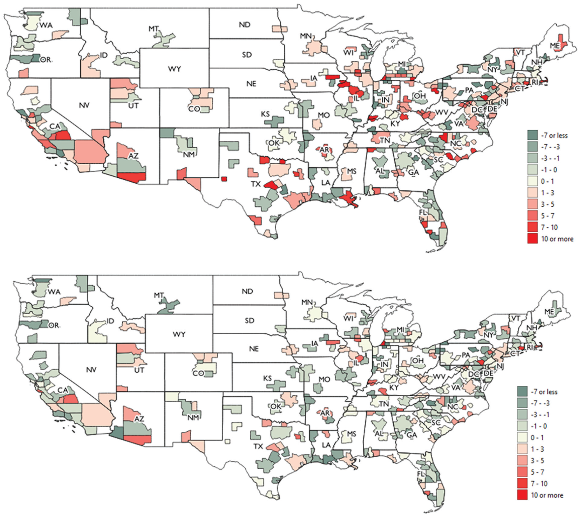
Changes in household joblessness (top) and contribution from polarization to changes in household joblessness (bottom) across metropolitan areas in Q1 2021.

The first thing the maps tell us is that both the change in household joblessness and the contribution from polarization varied widely across metropolitan areas. There are many areas, in which polarization reinforces the overall change. In Arizona, for example, Phoenix has low negative contribution of polarization and negative household joblessness. The neighboring Prescott Valley and Tucson have high positive contributions to very high increases in household joblessness. Yuma, in the west, shows a strong negative contribution to moderate household joblessness. But there are also areas in which polarization contributions and overall household joblessness diverge. Several areas in Wisconsin and Minnesota, for instance, have negative polarization contributions but still increases in household joblessness. This is not unexpected, as overall increases in individual joblessness can account for rising household joblessness. Yet there are also single areas with positive polarization contributions but overall decreases in household joblessness (e.g., Provo-Orem in Utah).

Figure 4 shows how changes in household joblessness (left-hand panels) and the contribution of polarization to these changes (right-hand panels) in Q1 2021 correlate with our three educational variables (measured as the prepandemic average of these variables in the respective metropolitan area). Overall, two things are noteworthy. First, as shown in Figure 3, there is ample variation across metropolitan areas in changes in household joblessness and the contribution of polarization. Second, correlations with educational variables are weak but indicative (in fact, correlations with any other sociodemographic variables in our data are weak). Correlations tend to be positive, except for educational levels showing a slight negative correlation with changes in household joblessness. Metropolitan areas with higher educational levels on average suffered slightly smaller increases in household joblessness. At the same time, the association with the contribution from polarization is positive, indicating that inequality in the distribution of jobs across households increased. For both educational heterogeneity and educational homogamy, we observe slight positive correlations with the contribution of polarization and slightly stronger positive correlations with changes in household joblessness. Thus, both educational factors are associated with an overall larger increase in household joblessness and greater inequality in the distribution of jobs as a cause of the larger increase.

Figure 4.

Bivariate correlations between changes in household joblessness (left-hand panels) and contribution from polarization to changes in household joblessness in Q1 2021 with educational levels, heterogeneity, and homogamy across metropolitan areas.

Overall, the decompositions illustrate a large increase in household joblessness compared with prepandemic levels in many metropolitan areas. By the end of 2021, household joblessness is close to prepandemic levels in many areas. Developments and the role of polarization varied strongly across areas. Correlations with educational variables indicate mostly weak associations that mostly align with our considerations of the moderating role of educational profiles. For a more systematic test of the expected moderating role of educational profiles of metropolitan areas, the following section shows the results from our panel regression models.

Fixed-Effects Panel Regressions of Household Joblessness and Polarization

In our multivariate models, we regress the change in household joblessness and the contribution from polarization to changes in household joblessness on our educational profiles fully interacted with a quarter indicator and adjusting for a battery of lagged covariates. In Figure 5 we display the predicted changes in household joblessness (left-hand panel) and the predicted contribution from polarization (right-hand panel) for all quarters since the onset of the pandemic for metropolitan areas with different educational profiles from our model. Our models include the educational profiles as time-variant variables (full models can be found in Tables A2 and A3 in the Appendix; figures are based on model 3, respectively). For the figures, we group areas by their prepandemic profiles so that the displayed predictions contain a fixed set of metropolitan areas. We choose combinations that show high or low levels of the three indicators as defined as being in the lowest third or the highest third of the distribution of the respective indicator before the pandemic (average over all quarters, 2016–2019). Two theoretically possible combinations do not exist empirically (low levels combined with low heterogeneity and high homogamy and high levels combined with high heterogeneity and low homogamy) and another two are evident in only few metropolitan areas: we show the results for areas with low levels, high heterogeneity, and low homogamy (n = 5) but omit areas with high levels combined with low heterogeneity and high homogamy (n = 1).²

Figure 5.

Predicted changes in household joblessness and contribution from polarization to changes in household joblessness across educational profiles.

The first clear pattern is that metropolitan areas with low educational levels show larger increases in household joblessness (left-hand panel). Immediately after the onset of the pandemic, areas with low educational levels see increases in household joblessness of about 5 percentage points, whereas areas with high levels see smaller increases of about 4 percentage points or even less than 3 percentage points. Whereas all areas see household joblessness decrease over the subsequent quarters, trajectories differ. Areas with high educational levels arrive at prepandemic levels of household joblessness by the end of 2021 when they combine high levels with low heterogeneity and low homogamy (17 metropolitan areas representing about 7.6 percent of the population in our sample) and at about a 1 percentage point increase when they have high heterogeneity and high homogamy (12 metropolitan areas representing about 18.5 percent of the population in our sample). Areas that combine low levels with low heterogeneity and low homogamy show the most distinct reduction in elevated household joblessness, arriving below 1 percentage points by Q4 2021 (11 metropolitan areas representing about 2.1 percent of our sample). Areas that combine low levels with high heterogeneity and high homogamy show a slightly delayed reduction, arriving at slightly above 1.5 percentage points by Q4 2021 (24 metropolitan areas representing 10.5 percent of the population in our sample). Areas with low levels, high heterogeneity, and low homogamy show a similar development except for a notable uptick in Q4 2021, which leaves them at an increase in household joblessness of almost 3 percentage points (5 metropolitan areas representing about 2.4 percent of the population in our sample).

The picture is more varied when inspecting how much changes in polarization contribute to the increase and subsequent decline in household joblessness across areas (right-hand panel). Given their low levels of household joblessness, polarization plays an outsize role in areas with high educational levels, high heterogeneity, and high homogamy, adding about 0.6 percentage points at the beginning of the pandemic and closing at a contribution of about 0.7 percentage points by the end of 2021. This positive contribution from changes in polarization counters higher individual employment levels compared with before the pandemic. Areas with high levels but low heterogeneity and homogamy fluctuate around a zero contribution from changes in polarization after an initial negative contribution. Compared with the overall changes in household joblessness, the standout finding for polarization is that in areas with low levels and low heterogeneity and homogamy the contribution from polarization is small and even negative in single instances. By contrast, in areas that combine low levels with either high heterogeneity and low homogamy or high heterogeneity and high homogamy, changes in polarization contribute notably more and are a central reason why overall increases in household joblessness do not return to prepandemic levels. Thus, although educational levels seem to make the largest difference when it comes to overall changes in household jobless, educational heterogeneity and homogamy play an important role when it comes to levels and change of polarization. On balance, there is some evidence indicating that lower heterogeneity and lower homogamy correlate with less (increase in) polarization.

We conduct several additional analyses to assess the robustness of our findings. First, we use alternative thresholds of our education measures to represent the educational profiles of metropolitan areas. Using the median to determine low and high values enables a look at all metropolitan areas (see Figure A3 in the Appendix). The overall changes and patterns resemble the ones presented here but, unsurprisingly, are generally more moderate and differences between combinations are smaller. Using values in the lowest and highest quartile reduces the number of represented areas and leads to more extreme differences (see Figure A4 in the Appendix). We also test how reducing the sample to households with at least one member aged 25 to 54 years changes our results (see Figure A5 in the Appendix). The main difference here is that polarization patterns follow more closely the development of overall household joblessness. Finally, we show how using alternative educational measures changes the results (see Figure A6 in the Appendix). Instead of years of schooling, here we use three levels of educational attainment to measure average educational levels, educational heterogeneity, and educational homogamy (for details, see note for Figure A6). Using alternative educational measures leads to different allocations of areas to educational profiles. For instance, some of the metropolitan areas we group as high educational level, high educational heterogeneity, and high educational homogamy in the main analysis are grouped as having high educational levels, high educational homogamy, but low educational heterogeneity when using educational attainment. As they represent different metropolitan areas, the results show some different patterns. But they confirm that changes in household joblessness differ strongly for educational levels, whereas the development of polarization is affected by heterogeneity and homogamy as well. We prefer the measures based on years in education because attainment measures mean a loss of information.

Conclusions

In this article, we set out to answer three questions. First, how did household joblessness develop in U.S. metropolitan areas during the COVID-19 economic crisis and how did it vary across local labor markets? Second, how much of this development and cross–labor market variation was simply due to rising numbers in individual joblessness, and how much was due to the unequal distribution of job loss across households (i.e., polarization)? Third, can we explain cross–labor market variation in changes in household joblessness and polarization with the educational profiles of these labor markets? We used monthly CPS data pooled in quarters for 204 metropolitan areas from 2016 to 2021. To answer the first two questions, we used a shift-share decomposition that broke down changes in household joblessness since the start of the pandemic into the contribution from individual joblessness, changes in household sizes, and polarization. We found a large increase in household joblessness during the pandemic. This moved largely in step with individual joblessness but positive polarization added a nontrivial amount. Moreover, variance across metropolitan areas was large in the initial increase in household joblessness, its subsequent development, and in the contribution from polarization. We used fixed-effects panel regressions on the level of metropolitan areas to answer our third question. Partly, the development of household joblessness and polarization aligned with our expectations about the educational profiles of metropolitan areas. Areas with low educational levels generally showed larger increases in household joblessness. Although overall household joblessness approximated prepandemic levels by the end of 2021, the contributions from polarization were more stable, indicating that the new equilibrium concentrated individual joblessness more strongly in households. Overall, areas with low educational levels, high educational heterogeneity, and low homogamy saw the largest contribution from higher polarization. But positive polarization also steadily contributed to elevated household joblessness in areas with high heterogeneity and high homogamy, be they combined with high or low levels. By contrast, areas with low or high educational levels combined with low heterogeneity and low homogamy saw almost no contributions from polarization, in some quarters even negative contributions (i.e., absorption of individual joblessness in households). Although these patterns align with our expectations, it has to be pointed out that much of the changes in household joblessness and polarization remain unexplained. No single variable in our battery of sociodemographic and economic covariates showed strong correlations with our outcomes either (compare Tables A2 and A3 in the Appendix).

Our analysis has some important limitations. First, we used CPS data and metropolitan areas because the CPS is the only available data source for analyzing household joblessness during the pandemic, as it publishes new data monthly. Metropolitan areas are the spatial unit to analyze local labor markets in the CPS with sufficient case numbers, but smaller case numbers for some metropolitan areas could lead to less robust findings. Although looking at metropolitan areas allowed us to extend existing research on U.S. geographic economic inequality, we intend to explore long-term trends in U.S. household joblessness using U.S. census and American Community Survey data in future work. Studies analyzing commuting zones usually use U.S. census and American Community Survey data, meaning that case numbers per spatial unit are also notably larger (e.g., Autor and Dorn 2013; VanHeuvelen and Copas 2019).

Second, because we analyzed metropolitan areas, we had to work with a very limited case number in our multivariate analysis. Our models included up to four-way interactions and a battery of covariates for which a sample of 204 metropolitan areas arguably yields not enough power. We were therefore able to cautiously describe differences in trends, but statistical tests of differences will have to be conducted in future work with larger samples. Again, analyzing commuting zones would provide a larger sample size of more than 700.

Third, our focus was on the level of metropolitan areas because polarization is intuitively a macro concept and because it enabled us to consider externalities of educational measures. However, future work analyzing individual level data could help us illustrate differences between households that accumulate employment risks more clearly. Finally, analyzing household joblessness during the COVID-19 pandemic might have limited generalizability because of the occupational distribution of job loss and idiosyncratic impacts on household dynamics. Future work might test our education-based explanation for prior economic downturns as well as long-term trends.

Overall, we might look at the development of household joblessness and interpret the return to prepandemic levels by the end of 2021 as good news. Although changes in polarization proved stickier in some areas, they are still relatively low in international comparison (Biegert and Ebbinghaus 2022; Gregg et al. 2008; Gregg and Wadsworth 2001). However, it took almost two years to arrive at prepandemic levels, meaning that an increased number of individuals experienced the hardships connected to living in a jobless household. Also, we need to remember that prepandemic levels still mean that about 10 percent of working-age adults in metropolitan areas live in households with no one working. Moreover, both household joblessness and polarization are markedly above the national average in some metropolitan areas. Because household joblessness increased by up to 5 percentage points nationally and by more than 15 percentage points in some metropolitan areas, an increased share of the population lived at a higher risk for poverty. In our sample, jobless households without children showed a poverty risk of about 65 percent, and almost 75 percent of jobless households with children were at risk for poverty (compared with about 15 percent for employed households without children and 28 percent of employed households with children) (see Figure A7 in the Appendix). Notably, poverty risks of jobless households with children increased in 2021 after a brief drop in 2019 and 2020. Thus, even though state support was generous in the first phase of the pandemic, it was cut down soon again, leaving jobless households and particularly those with children highly vulnerable to immediate adverse impacts of poverty. That the accumulation of individual employment risks that shows in household joblessness and especially in the polarization of household joblessness is concentrated in some metropolitan areas is important for understanding the concentration of poverty in geographical pockets of the United States (Jargowsky 1996; Kneebone et al. 2011; Wilson 1997).

Experiencing household joblessness during the pandemic and after is also likely to leave household members with scars that transcend the impact of poverty (Curry et al. 2022; Ermisch et al. 2004; Mooi-Reci et al. 2020). Besides documenting the challenge of household joblessness in the United States, our study provided an explanation of variation in household joblessness and polarization across labor markets that went beyond coarse models of welfare regimes and dominant family models (Biegert and Ebbinghaus 2022; Corluy and Vandenbroucke 2017; Gregg et al. 2008). It connects work that highlights skills divides to explain growing economic inequality in the United States with the literature focusing on racial divides to explain the concentration of urban poverty (Jargowsky 1996; Moller et al. 2009; Reardon and Bischoff 2011; VanHeuvelen and Copas 2019; Wilson 1987). Because high household joblessness implies an additional dimension of accumulated risks, further developing the education-based model might prove helpful in identifying geographic pockets of entrenched spatial economic disadvantage.

Footnotes

Appendix

Table A3.

Panel Fixed-Effects Regression Models of Contribution from Polarization to Changes in Household Joblessness.

	Model 1 (No Interactions)			Model 2 (Two-Way Interactions)			Model 3 (Four-Way Interactions)
	β	SE	p	β	SE	p	β	SE	p
Edu. lev.	−3.087	1.566	.050	−7.713	2.549	.003	430.009	216.387	.048
Edu. het.	−.366	2.677	.892	−9.798	5.438	.073	269.931	159.123	.091
Edu. hom.	.185	.959	.847	−.449	2.326	.847	408.119	228.351	.075
Q2 2020 (ref.)
Q3 2020	.199	.238	.403	−8.746	6.665	.191	442.793	203.929	.031
Q4 2020	.004	.269	.989	−13.060	8.126	.110	315.999	223.081	.158
Q1 2021	−.112	.283	.692	−17.968	8.181	.029	93.537	216.806	.667
Q2 2021	.293	.258	.257	−21.051	7.239	.004	103.568	167.879	.538
Q3 2021	.149	.257	.562	−13.108	6.873	.058	149.692	162.142	.357
Q4 2021	.002	.288	.995	−8.076	7.782	.301	155.571	167.417	.354
% Black (lagged)	−1.379	2.524	.585	−1.273	2.461	.606	−.715	2.428	.769
% Hispanic (lagged)	1.872	2.232	.403	2.026	2.294	.378	2.667	2.367	.261
% migrants (lagged)	−.081	1.804	.964	−.598	1.784	.738	−1.056	1.862	.571
% single HH heads (lagged)	.416	1.522	.785	.460	1.502	.760	−.044	1.484	.976
% ≥65 (lagged)	1.545	2.990	.606	1.636	3.031	.590	1.920	3.015	.525
Median eq. HH income (lagged)	.000	.000	.677	.000	.000	.698	.000	.000	.687
% pub. admin. (lagged)	2.351	4.416	.595	1.651	4.504	.714	1.244	4.626	.788
% manufacturing (lagged)	−6.965	3.167	.029	−7.177	3.109	.022	−6.740	3.173	.035
% FIRE (lagged)	−6.423	3.963	.107	−5.934	3.940	.134	−7.637	3.918	.053
% other services	−3.073	1.909	.109	−3.127	1.904	.102	−3.594	1.911	.061
% city dwellers	2.251	1.628	.168	2.275	1.616	.161	2.381	1.512	.117
Total population size	.000	.000	.770	.000	.000	.764	.000	.000	.938
Q2 2020 × edu. lev. (ref.)
Q3 2020 × edu. lev.				5.092	2.707	.061	−684.554	307.671	.027
Q4 2020 × edu. lev.				5.832	3.322	.081	−441.866	314.573	.162
Q1 2021 × edu. lev.				8.154	3.390	.017	−180.713	309.391	.560
Q2 2021 × edu. lev.				6.986	2.794	.013	−222.128	228.184	.331
Q3 2021 × edu. lev.				2.875	2.632	.276	−279.514	224.510	.215
Q4 2021 × edu. lev.				5.817	3.183	.069	−329.697	253.873	.196
Q2 2020 × edu. het. (ref.)
Q3 2020 × edu. het.				6.229	5.061	.220	−431.461	204.358	.036
Q4 2020 × edu. het.				8.262	7.294	.259	−312.870	221.112	.159
Q1 2021 × edu. het.				10.236	6.294	.105	−126.032	214.937	.558
Q2 2021 × edu. het.				14.957	5.694	.009	−112.628	169.105	.506
Q3 2021 × edu. het.				10.644	5.415	.051	−136.502	163.856	.406
Q4 2021 × edu. het.				4.162	6.458	.520	−145.671	169.312	.391
Q2 2020 × edu. hom. (ref.)
Q3 2020 × edu. hom.				−1.484	3.268	.650	−620.754	302.835	.042
Q4 2020 × edu. hom.				1.041	2.806	.711	−432.990	359.564	.230
Q1 2021 × edu. hom.				3.008	3.323	.367	−245.602	297.015	.409
Q2 2021 × edu. hom.				1.900	2.798	.498	−161.340	243.723	.509
Q3 2021 × edu. hom.				.353	2.820	.901	−211.624	237.422	.374
Q4 2021 × edu. hom.				−.108	3.268	.974	−181.768	243.747	.457
Edu. lev. × edu. het.							−425.715	219.419	.054
Q2 2020 × edu. lev. × edu. het. (ref.)
Q3 2020 × edu. lev. × edu. het.							668.736	307.909	.031
Q4 2020 × edu. lev. × edu. het.							438.897	313.141	.163
Q1 2021 × edu. lev. × edu. het.							227.471	306.958	.460
Q2 2021 × edu. lev. × edu. het.							232.342	232.637	.319
Q3 2021 × edu. lev. × edu. het.							255.761	228.071	.263
Q4 2021 × edu. lev. × edu. het.							310.472	255.570	.226
Edu. lev. × edu. hom.							−628.008	319.819	.051
Q2 2020 × edu. lev. × edu. hom. (ref.)
Q3 2020 × edu. lev. × edu. hom.							952.083	462.313	.041
Q4 2020 × edu. lev. × edu. hom.							583.956	512.872	.256
Q1 2021 × edu. lev. × edu. hom.							418.879	431.045	.332
Q2 2021 × edu. lev. × edu. hom.							313.140	339.282	.357
Q3 2021 × edu. lev. × edu. hom.							379.664	332.720	.255
Q4 2021 × edu. lev. × edu. hom.							411.628	373.347	.272
Edu. het. × edu. hom.							−397.727	232.001	.088
Q2 2020 × edu. het. × edu. hom. (ref.)
Q3 2020 × edu. het. × edu. hom.							599.980	305.892	.051
Q4 2020 × edu. het. × edu. hom.							423.971	357.504	.237
Q1 2021 × edu. het. × edu. hom.							287.549	298.853	.337
Q2 2021 × edu. het. × edu. hom.							169.395	248.033	.495
Q3 2021 × edu. het. × edu. hom.							188.348	242.775	.439
Q4 2021 × edu. het. × edu. hom.							161.000	249.417	.519
Edu. lev. × edu. het. × edu. hom.							612.072	326.629	.062
Q2 2020 × edu. lev. × edu. het. × edu. hom. (ref.)
Q3 2020 × edu. lev. × edu. het. × edu. hom.							−922.708	465.800	.049
Q4 2020 × edu. lev. × edu. het. × edu. hom.							−573.318	512.332	.264
Q1 2021 × edu. lev. × edu. het. × edu. hom.							−479.286	434.065	.271
Q2 2021 × edu. lev. × edu. het. × edu. hom.							−320.463	349.105	.360
Q3 2021 × edu. lev. × edu. het. × edu. hom.							−339.223	342.072	.323
Q4 2021 × edu. lev. × edu. het. × edu. hom.							−374.222	380.004	.326
Constant	2.995	3.667	.415	16.392	6.888	.018	−271.070	158.135	.088
n	1,428			1,428			1,428
N	204			204			204

Note: edu. het. = educational heterogeneity; edu. hom. = educational homogamy; edu. lev. = educational level; eq. = equivalent; FIRE = finance, insurance, and real estate; HH = household; pub. admin. = public administration; ref. = reference.

Acknowledgements

We are thankful for helpful insights from the LSE Social Policy Quantitative Reading group, Nathan Wilmers and the audience at the American Sociological Association annual conference in Los Angeles, the audience at the Oxford Nuffield College Sociology Seminar Series, the audience at the RC28 Spring Conference in London, and the audience at the ECSR conference in Amsterdam. We are also grateful for constructive comments from the two anonymous reviewers and the editors at Socius.

Funding

The author(s) disclosed receipt of the following financial support for the research, authorship, and/or publication of this article: This research resulted from a grant supported by the LSE’s Research Support Fund in 2021.

ORCID iDs

Thomas Biegert

Berkay Özcan

1

Replication files can be found at DOI 10.17605/OSF.IO/6CR3N.

2

Figure A2 in the shows the distribution of metropolitan areas over educational profiles, plotting the correlation between educational heterogeneity and educational homogamy for three educational levels.

Author Biographies

Thomas Biegert is an assistant professor of social policy at the London School of Economics and Political Science. His research on social inequalities in labor markets has been published in journals such as American Sociological Review, Socio-economic Review, European Sociological Review, and the Journal of European Social Policy.

Berkay Özcan is an associate professor in the Department of Social Policy and the School of Public Policy at the London School of Economics. Before joining London School of Economics, he worked as a postdoctoral researcher at Yale University. He has held visiting researcher positions at Princeton University (2006), Essex University (2007), and University College London (2017). He is an external research fellow at University College London’s Center for Research and Analysis on Migration. He was awarded a Jemolo Fellowship at the Nuffield College of the University of Oxford (2015). He studies the relationship between demographic processes and economic outcomes. He has published in prominent journals in economics, demography, and sociology, such as Annual Review of Sociology, Demography, the Proceedings of the National Academy of Sciences, the Journal Human Resources, and European Economic Review, among others.

Magdalena Rossetti-Youlton is a PhD candidate at the London School of Economics and Political Science. Her research focuses on poverty, spatial inequalities, and household composition. She has more than 10 years of experience working in the public sector, international organizations, and research institutes in policy areas such as employment, health, education, taxation, and urban development.

References

Allison

Paul D.

2009. Fixed Effects Regression Models. Thousand Oaks, CA: Sage.

Alon

Titan

Doepke

Matthias

Olmstead-Rumsey

Jane

Tertilt

Michèle

. 2020. “The Impact of COVID-19 on Gender Equality.” NBER Working Paper No. 26947. Cambridge, MA: National Bureau of Economic Research.

Autor

David H.

Dorn

David

. 2013. “The Growth of Low-Skill Service Jobs and the Polarization of the US Labor Market.” American Economic Review 103(5):1553–97.

Biegert

Thomas

Ebbinghaus

Bernhard

. 2022. “Accumulation or Absorption? Changing Disparities of Household Non-employment in Europe during the Great Recession.” Socio-economic Review 20(1):141–68.

Bitler

Marianne

Hoynes

Hilary

. 2015. “Living Arrangements, Doubling Up, and the Great Recession: Was This Time Different?” American Economic Review 105(5):166–70.

Blossfeld

Hans-Peter

Buchholz

Sandra

. 2009. “Increasing Resource Inequality among Families in Modern Societies: The Mechanisms of Growing Educational Homogamy, Changes in the Division of Work in the Family and the Decline of the Male Breadwinner Model.” Journal of Comparative Family Studies 40(4):603–15.

Brand

Jennie E.

2015. “The Far-Reaching Impact of Job Loss and Unemployment.” Annual Review of Sociology 41:359–75.

Breen

Richard

Salazar

Leire

. 2011. “Educational Assortative Mating and Earnings Inequality in the United States.” American Journal of Sociology 117(3):808–43.

Brooks

Matthew M.

Mueller

J. Tom

Thiede

Brian C.

2021. “Rural-Urban Differences in the Labor-Force Impacts of COVID-19 in the United States.” Socius: Sociological Research for a Dynamic World. doi:10.1177/23780231211022094.

10.

Cho

Seung Jin

Lee

Jun Yeong

Winters

John V.

2021. “Employment Impacts of the COVID-19 Pandemic across Metropolitan Status and Size.” Growth and Change 52(4):1958–96.

11.

Collins

Caitlyn

Landivar

Liana Christin

Ruppanner

Leah

Scarborough

William J.

2021. “COVID-19 and the Gender Gap in Work Hours.” Gender, Work & Organization 28(S1):101–12.

12.

Corluy

Vincent

Vandenbroucke

Frank

. 2017. “Individual Employment, Household Employment and Risk of Poverty in the EU. A Decomposition Analysis.” Pp. 279–98 in Monitoring Social Inclusion in Europe, edited by Atkinson

A. B.

Guio

A.-C.

Marlier

Luxembourg City, Luxembourg: Eurostat.

13.

Costa

Dora L.

Kahn

Matthew E.

2000. “Power Couples: Changes in the Locational Choice of the College Educated, 1940–1990.” Quarterly Journal of Economics 115(4):1287–315.

14.

Couch

Kenneth A.

Fairlie

Robert W.

Huanan

. 2020. “Early Evidence of the Impacts of COVID-19 on Minority Unemployment.” Journal of Public Economics 192:104287.

15.

Curry

Matthew

Mooi-Reci

Irma

Wooden

Mark

. 2019. “Parental Joblessness and the Moderating Role of a University Degree on the School-to-Work Transition in Australia and the United States.” Social Science Research 81:61–76.

16.

Curry

Matthew

Mooi-Reci

Irma

Wooden

Mark

. 2022. “Intergenerationally Penalized? The Long-Term Wage Consequences of Parental Joblessness.” Social Science Research 103:102650.

17.

Dalton

Michael

. 2020. “Labor Market Effects of Local Spread of COVID-19: U.S. Bureau of Labor Statistics.” BLS Working Paper 254. Washington, DC: Bureau of Labor Statistics.

18.

de Graaf-Zijl

Marloes

Nolan

Brian

. 2011. “Household Joblessness and Its Impact on Poverty and Deprivation in Europe.” Journal of European Social Policy 21(5):413–31.

19.

Dias

Felipe A.

2021. “The Racial Gap in Employment and Layoffs during COVID-19 in the United States: A Visualization.” Socius: Sociological Research for a Dynamic World. doi:10.1177/2378023120988397.

20.

Eika

Lasse

Mogstad

Magne

Zafar

Basit

. 2019. “Educational Assortative Mating and Household Income Inequality.” Journal of Political Economy 127(6):2795–835.

21.

Ermisch

John

Francesconi

Marco

Pevalin

David J.

2004. “Parental Partnership and Joblessness in Childhood and Their Influence on Young People’s Outcomes.” Journal of the Royal Statistical Society: Series A (Statistics in Society) 167(1):69–101.

22.

Essletzbichler

Jürgen

. 2015. “The Top 1% in U.S. Metropolitan Areas.” Applied Geography 61:35–46.

23.

Faccini

Renato

Melosi

Leonardo

Miles

Russell

. 2022. “The Effects of the ‘Great Resignation’ on Labor Market Slack and Inflation.” Chicago Fed Letter (No. 465). Chicago: Federal Reserve Bank of Chicago.

24.

Farber

Henry S.

2005. “What Do We Know about Job Loss in the United States? Evidence from the Displaced Workers Survey, 1984–2004.” Economic Perspectives 29(2):13–28.

25.

Farber

Henry S.

2015. “Job Loss in the Great Recession and Its Aftermath: U.S. Evidence from the Displaced Workers Survey.” NBER Working Paper No. 21216. Cambridge, MA: National Bureau of Economic Research.

26.

Flood

Sarah

King

Miriam

Renae

Rodgers

Ruggles

Steven

Warren

Robert J.

Westberry

Michael

. 2021. “Integrated Public Use Microdata Series, Current Population Survey: Version 7.0.” Minneapolis, MN: IPUMS.

27.

Fossett

Mark A.

Kiecolt

K. Jill

. 1993. “Mate Availability and Family Structure among African Americans in U. S. Metropolitan Areas.” Journal of Marriage and Family 55(2):288–302.

28.

Fowler

Christopher S.

Jensen

Leif

. 2020. “Bridging the Gap between Geographic Concept and the Data We Have: The Case of Labor Markets in the USA.” Environment and Planning A: Economy and Space 52(7):1395–1414.

29.

García

Daniel

Paciorek

Andrew

. 2022. “The Remarkable Recent Rebound in Household Formation and the Prospects for Future Housing Demand.” FEDS Notes. Washington, DC: Board of Governors of the Federal Reserve System.

30.

Gesthuizen

Maurice

Solga

Heike

Künster

Ralf

. 2011. “Context Matters: Economic Marginalization of Low-Educated Workers in Cross-National Perspective.” European Sociological Review 27(2):264–80.

31.

Glaeser

Edward L.

Saiz

Albert

. 2004. “The Rise of the Skilled City.” Brookings-Wharton Papers on Urban Affairs 2004:47–105.

32.

Greenwood

Jeremy

Guner

Nezih

Kocharkov

Georgi

Santos

Cezar

. 2014. “Marry Your Like: Assortative Mating and Income Inequality.” American Economic Review 104(5):348–53.

33.

Gregg

Paul

Scutella

Rosanna

Wadsworth

Jonathan

. 2008. “Reconciling Workless Measures at the Individual and Household Level. Theory and Evidence from the United States, Britain, Germany, Spain and Australia.” Journal of Population Economics 23(1):139–67.

34.

Gregg

Paul

Wadsworth

Jonathan

. 2001. “Everything You Ever Wanted to Know about Measuring Worklessness and Polarization at the Household Level but Were Afraid to Ask.” Oxford Bulletin of Economics and Statistics 63(s1):777–806.

35.

Iceland

John

Hernandez

Erik

. 2017. “Understanding Trends in Concentrated Poverty: 1980–2014.” Social Science Research 62:75–95.

36.

Jaeger

David A.

1997. “Reconciling the Old and New Census Bureau Education Questions: Recommendations for Researchers.” Journal of Business & Economic Statistics 15(3):300–309.

37.

Jargowsky

Paul A.

1996. “Take the Money and Run: Economic Segregation in U.S. Metropolitan Areas.” American Sociological Review 61(6):984.

38.

Kesler

Christel

Bash

Sarah

. 2021. “A Growing Educational Divide in the COVID-19 Economy Is Especially Pronounced among Parents.” Socius: Sociological Research for a Dynamic World. doi:10.1177/2378023120979804.

39.

Klein

Markus

. 2015. “The Increasing Unemployment Gap between the Low and High Educated in West Germany. Structural or Cyclical Crowding-Out?” Social Science Research 50:110–25.

40.

Kneebone

Elizabeth

Nadeau

Carey

Berube

Alan

. 2011. “The Re-emergence of Concentrated Poverty: Metropolitan Trends in the 2000s.” Washington, DC: Metropolitan Policy Program at Brookings.

41.

Krivo

Lauren J.

Peterson

Ruth D.

Rizzo

Helen

Reynolds

John R.

1998. “Race, Segregation, and the Concentration of Disadvantage: 1980–1990.” Social Problems 45(1):61–80.

42.

Angran

Wallace

Michael

Hyde

Allen

. 2019. “Degrees of Inequality: The Great Recession and the College Earnings Premium in U.S. Metropolitan Areas.” Social Science Research 84:102342.

43.

Liao

Tim F.

Özcan

Berkay

. 2013. “Family Forms among First- and Second-Generation Immigrants in Metropolitan America, 1960–2009.” Pp. 223–254 in Immigrant Adaptation in Multi-Ethnic Societies: Canada, Taiwan, and the United States, edited by Fong

Chiang

L.-H.N.

Denton

Oxford, UK: Routledge.

44.

Liu

Yujia

Grusky

David B.

2013. “The Payoff to Skill in the Third Industrial Revolution.” American Journal of Sociology 118(5):1330–74.

45.

Massey

Douglas S.

Eggers

Mitchell L.

1990. “The Ecology of Inequality: Minorities and the Concentration of Poverty, 1970-1980.” American Journal of Sociology 95(5):1153–88.

46.

Massey

Douglas S.

Eggers

Mitchell L.

1993. “The Spatial Concentration of Affluence and Poverty during the 1970s.” Urban Affairs Quarterly 29(2):299–315.

47.

Massey

D. S.

Shibuya

1995. “Unraveling the Tangle of Pathology: The Effect of Spatially Concentrated Joblessness on the Well-Being of African Americans.” Social Science Research 24(4):352–66.

48.

Mincer

Jacob

. 1970. “The Distribution of Labor Incomes: A Survey with Special Reference to the Human Capital Approach.” Journal of Economic Literature 8(1):1–26.

49.

Moller

Stephanie

Alderson

Arthur S.

Nielsen

François

. 2009. “Changing Patterns of Income Inequality in U.S. Counties, 1970–2000.” American Journal of Sociology 114(4):1037–1101.

50.

Mooi-Reci

Irma

Wooden

Mark

Curry

Matthew

. 2020. “The Employment Consequences of Growing up in a Dual-Parent Jobless Household: A Comparison of Australia and the United States.” Research in Social Stratification and Mobility 68:100519.

51.

Mulligan

Gordon F.

2023. “Economic Vulnerability in US Metropolitan Areas.” Annals of Regional Science 70(1):29–53.

52.

Mulligan

Gordon F.

Reid

Neil

Moore

Michael S.

2014. “A Typology of Metropolitan Labor Markets in the US.” Cities 41:S12–29.

53.

Nielsen

Francois

Alderson

Arthur S.

1997. “The Kuznets Curve and the Great U-Turn: Income Inequality in U.S. Counties, 1970 to 1990.” American Sociological Review 62(1):12–33.

54.

Quillian

Lincoln

. 2003. “How Long Are Exposures to Poor Neighborhoods? The Long-Term Dynamics of Entry and Exit from Poor Neighborhoods.” Population Research and Policy Review 22(3):221–49.

55.

Quillian

Lincoln

. 2012. “Segregation and Poverty Concentration: The Role of Three Segregations.” American Sociological Review 77(3):354–79.

56.

Raymo

James M.

Xie

. 2000. “Temporal and Regional Variation in the Strength of Educational Homogamy.” American Sociological Review 65(5):773–81.

57.

Reardon

Sean F.

Bischoff

Kendra

. 2011. “Income Inequality and Income Segregation.” American Journal of Sociology 116(4):1092–153.

58.

Riddell

W. Craig

Song

Xueda

. 2011. “The Impact of Education on Unemployment Incidence and Re-employment Success: Evidence from the U.S. Labour Market.” Labour Economics 18(4):453–63.

59.

Sampson

Robert J.

1987. “Urban Black Violence: The Effect of Male Joblessness and Family Disruption.” American Journal of Sociology 93(2):348–82.

60.

Sassen

Saskia

. 1990. “Economic Restructuring and the American City.” Annual Review of Sociology 16:465–90.

61.

Schwartz

Christine R.

2010. “Earnings Inequality and the Changing Association between Spouses’ Earnings.” American Journal of Sociology 115(5):1524–57.

62.

Schwartz

Christine R.

Mare

Robert D.

2005. “Trends in Educational Assortative Marriage from 1940 to 2003.” Demography 42(4):621–46.

63.

Scutella

Rosanna

Wooden

Mark

. 2004. “Jobless Households in Australia: Incidence, Characteristics and Financial Consequences.” Economic and Labour Relations Review 14(2):187–207.

64.

South

Scott J.

Crowder

Kyle

. 2010. “Neighborhood Poverty and Nonmarital Fertility: Spatial and Temporal Dimensions.” Journal of Marriage and Family 72(1):89–104.

65.

South

Scott J.

Crowder

Kyle D.

1999. “Neighborhood Effects on Family Formation: Concentrated Poverty and beyond.” American Sociological Review 64(1):113–32.

66.

South

Scott J.

Lloyd

Kim M.

1992. “Marriage Opportunities and Family Formation: Further Implications of Imbalanced Sex Ratios.” Journal of Marriage and Family 54(2):440–51.

67.

Ultee

Wout

Dessens

Jos

Jansen

Wim

. 1988. “Why Does Unemployment Come in Couples? An Analysis of (Un)Employment and (Non)Employment Homogamy Tables for Canada, the Netherlands and the United States in the 1980s.” European Sociological Review 4(2):111–22.

68.

U.S. Census Bureau. 2022. “Urban Areas Facts.” Retrieved July 19, 2022. https://www.census.gov/programs-surveys/geography/guidance/geo-areas/urban-rural/ua-facts.html.

69.

VanHeuvelen

Tom

Copas

Katherine

. 2019. “The Geography of Polarization, 1950 to 2015.” RSF: The Russell Sage Foundation Journal of the Social Sciences 5(4):77–103.

70.

Wagmiller

Robert L.

2007. “Race and the Spatial Segregation of Jobless Men in Urban America.” Demography 44(3):539–62.

71.

Wallace

Michael

Brady

David

. 2001. “The Next Long Swing: Spatialization, Technocratic Control, and the Restructuring of Work at the Turn of the Century.” Pp. 101–33 in Sourcebook of Labor Markets: Evolving Structures and Processes, Plenum Studies in Work and Industry, edited by Berg

Kalleberg

A. L.

Boston: Springer.

72.

Wiemers

Emily E.

2014. “The Effect of Unemployment on Household Composition and Doubling Up.” Demography 51(6):2155–78.

73.

Wilson

William Julius

. 1987. The Truly Disadvantaged: The Inner City, the Underclass, and Public Policy. Chicago: University of Chicago Press.

74.

Wilson

William Julius

. 1997. When Work Disappears: The World of the New Urban Poor. New York: Knopf.

75.

Winters

John V.

2013. “Human Capital Externalities and Employment Differences across Metropolitan Areas of the USA.” Journal of Economic Geography 13(5):799–822.

Household Joblessness in U.S. Metropolitan Areas during the COVID-19 Pandemic: Polarization and the Role of Educational Profiles

Abstract

Keywords

Background

Polarization in Household Joblessness Because of Accumulation and Absorption

Educational Profiles of Labor Markets

Context: The COVID-19 Economic Crisis in U.S. Metropolitan Areas

CPS 2016 to 2021 1

Data and Sample

Variables

Analytical Strategy

Shift-Share Decomposition

Metropolitan Area–Level Panel Fixed-Effects Models

Results

Household Joblessness and Its Decomposition in All U.S. Metropolitan Areas Combined

Variation across Metropolitan Areas

Fixed-Effects Panel Regressions of Household Joblessness and Polarization

Conclusions

Footnotes

Appendix

Acknowledgements

Funding

ORCID iDs

1

2

Author Biographies

References

CPS 2016 to 2021¹