Extreme and Inconsistent: A Case-Oriented Regression Analysis of Health,Inequality,and Poverty

Abstract

A methodological paradox characterizes macro-comparative research: it routinely violates the assumptions underlying its dominant method, multiple regression analysis. Comparative researchers have substantive interest in cases, but cases are largely rendered invisible in regression analysis. Researchers seldom recognize the mismatch between the goals of macro-comparative research and the demands of regression methods, and sometimes they end up engaging in strenuous disputes over particular variable effects. A good example is the controversial relationship between income inequality and health. Here, the authors offer an innovative method that combines variable-oriented and case-oriented approaches by turning ordinary least squares regression models “inside out.” The authors estimate case-specific contributions to regression coefficient estimates. They reanalyze data on income inequality, poverty, and life expectancy across 20 affluent countries. Multiple model specifications are dependent primarily on two countries with values on the outcome that are extreme in magnitude and inconsistent with conventional theoretical expectations.

Macro-comparative research is a sociological micro-world, which mirrors some of the contradictions and tensions that animate sociology as a discipline. Case-oriented and variable-oriented researchers engage a long-standing debate that recurrently gains prominence (Clausen and Mjoset 2007; Goertz and Mahoney 2012; Goldthorpe 1997; Kenworthy 2007; King, Keohane, and Verba 1994; Ragin 1987, 2000, 2008; Rubinson 2019; Shalev 2007; Verba 1967). With a degree of approximation, one can summarize the positions as follows. Case-oriented researchers claim to pursue a distinctive approach to social science regulated by a specific set of assumptions (Ragin 1997). Variable-oriented researchers, instead, suggest that case-oriented analysis can be improved by adhering more strictly to quantitative standards (King et al. 1994). Proponents of the latter persuasion are arguably leading the race, as demonstrated by the predominance of quantitative studies published in sociological journals. However, we argue that in recognizing the underlying logic that applies to both qualitative and quantitative analysis, that is, the logic of inference (King et al. 1994:3), many might fail to recognize a second common underlying logic, that is, the logic of case contribution. This latter logic is the one we introduce in this article, while showing how it can enrich usual multiple regression methods as applied in comparative research.

This logic of case contribution is particularly relevant for studies that base statistical inference on a small sample of nonindependent observations. Furthermore, we argue that, considering the logic of case contribution, it should be possible to make sense of some cyclical inconsistencies in findings, which at times tend to provoke disputes among researchers over their favored predictors. Here, we propose a methodological approach that moves both the logic of inference and the logic of case contribution to the forefront of the analysis. After estimating conventional regression models, we illustrate a procedure that is able to turn the regression “inside out,” to show the exact contribution of each case to each regression coefficient and to identify unusual cases. We apply this framework to an influential and rather controversial topic, that is, the relationship between income inequality and health.

Background: Macro-comparative Analysis and Multiple Regression Analysis

Macro-comparative analyses of social policy, political economy, and welfare regimes routinely use a common methodology, multiple regression analysis, whose assumptions are constantly violated in small-n comparisons (Shalev 2007). Aside from statistical limitations, one can argue that the major issue here is that multiple regression analysis tends to make invisible exactly what represents the focus of comparative investigation, that is, the cases. Scholars have proposed a number of alternatives, such as low-tech cross-tabular analysis, factor analysis, cluster analysis (Shalev 2007), and qualitative comparative analysis, in both its binary and fuzzy-set versions (Ragin 1987, 2000, 2008). Although all these techniques have virtues, they have all, to varying degrees, failed to become completely mainstream, at least in American sociology, which adopted statistical analysis as a marker of scientific rigor (Camic and Xie 1994; Leahey 2005; Liao 2014).

Although some comparative analysists advocate for abandoning regression techniques altogether, others believe that the issue is not the method itself but its implementation; in fact, “statistical analysis is used atrociously in a lot, if not most, comparative social science” (Scruggs 2007:310). Kenworthy (2007) proposed a plan to improve the use of multiple regression in comparative studies that involves more transparency, graphical presentation of the results, and more attention to the direction, magnitude, and robustness of coefficients. These strategies represent an improvement but might still fail to make cases visible. In fact, as Kenworthy noted, “in the prototypical quantitative macro-comparative article, the regressions are the starting and ending point of the analysis. I would like to see more papers in which regression is used to inform discussion of cases” (p. 349).

Breiger and colleagues (Breiger et al. 2011; Breiger and Melamed 2014; Melamed, Breiger, and Schoon 2012; Melamed, Schoon, et al. 2012) took on this challenge and developed a methodology that allows researchers to uncover a variety of stories lying underneath regression analysis. In fact, researchers can first estimate a traditional regression model and then turn it “inside out” to show case-specific contributions to coefficient estimates. This method factually bridges quantitative and qualitative methods and in this sense overcomes the hegemonic narrative of regression analysis. We apply this approach to a study of income inequality, poverty, and health, whose literature we now briefly review.

Inequality and Health

In the 1990s a series of articles published in the British Medical Journal (Kaplan et al. 1996; Kennedy et al. 1998; Kennedy, Kawachi, and Prothrow-Stith 1996; Wilkinson 1992), following a pioneer study in the late 1970s (Rodgers 1979), showed that aggregate levels of income inequality correlated with measures of population health, both across affluent countries and across the U.S. states, even after controlling for a number of factors, such as median income and poverty rates. The argument that inequality makes us sick by getting under our skin was powerful, and it resonated with ideas and evidence produced in an “enormous and well-developed body of social science” (Beckfield and Krieger 2009:153), which is characterized by large numbers of publications that report the negative consequences of economic inequalities (Jencks 2002).

In a nutshell, the income inequality hypothesis (IIH) states that in the affluent world, income inequality harms population health, net of other social determinants of health. Hundreds of studies have tested the IIH, using a variety of methods (Leigh et al. 2009; Mullahy, Robert, and Wolfe 2008). Ecological comparisons at national and subnational levels are particularly popular, because the IIH suggests that average income inequality is associated with average population health. In fact, the book that moved the IIH from exclusively academic debate into a larger public and political conversation, The Spirit Level (Wilkinson and Pickett 2009), also presents ecological comparisons.

After initial enthusiasm, the IIH gained a fair number of critics (Avendano and Hessel 2015; Beckfield 2004; Goldthorpe 2010; Lynch et al. 2004). One question is whether income inequality is actually associated with health. In fact, reviews estimate that 30 percent of published evidence does not support the IIH (Pickett and Wilkinson 2015; Wilkinson and Pickett 2006). Another issue is how to interpret the association. Two narratives emerged (Lynch et al. 2000). The first proposes a psychological interpretation of the relationship: inequality increases status anxiety, which turns into chronic stress, which leads to poor health. The second considers income inequality as part of a cluster of neomaterial conditions (e.g., poverty, public investment, welfare) that all contribute to shaping population health. One recent study tried a different approach: instead of playing inequality and poverty against each other, Rambotti (2015) investigated whether they interact. Here, we reproduce this analysis and then turn it “inside out,” examining the contribution of each case (national society) to the regression coefficients, and this leads us to important findings that were not anticipated in the earlier research.

Data

We apply this framework to data on income inequality, poverty, and life expectancy in 20 rich countries. Data on income inequality and health come from the influential book discussed above, The Spirit Level (Wilkinson and Pickett 2009). We briefly describe the data.

The measure of inequality is the p80/p20 income percentile ratio, the ratio of the income of those in the 80th percentile of the income distribution to those in the 20th percentile (from the United Nations Human Development Report, 2003–2006 average). The measure of poverty is the percentage of people living under 40 percent of the median household income in the respective country, provided by the Luxembourg Income Study. The time period is 2003 to 2006, with two exceptions: Belgium (2000) and Japan (2008). The measure of life expectancy comes from the United Nations Human Development Report. The sample was determined by removing countries with populations less than 3 million from the 50 wealthiest countries, as determined by the World Bank (Wilkinson and Pickett 2009). Countries not reported in the Luxembourg Income Study project were also excluded, leading to a sample size of 20. Table 1 shows the descriptive statistics.

Table 1.

Descriptive Statistics.

Variable	Mean	SD
Life expectancy	78.68	1.10
Income inequality (p80/p20 ratio)	5.50	1.33
Poverty (proportion living at <40% of median income)	5.51	2.71
Income inequality × poverty	32.63	23.01

One important question concerns the relationship between income inequality and poverty. Although it is intuitive that income inequality and poverty are to some extent dependent on each other, research has shown that they are two distinct phenomena, which are distinguishable both on the conceptual and the empirical level. For a detailed discussion, see Rambotti (2015), in particular section 3. For what concerns the present study, it suffices to say that the correlation between income inequality and poverty as measured here (respectively, the p80/p20 ratio and the percentage of the population living below 40 percent of the median income) is .67. This is a strong and positive correlation, in line with the known fact that inequality and poverty are dependent on each other, but it is low enough to affirm that the two constructs are not identical. In fact, one can assume that these two measures would give different results if used as predictors in a regression analysis, and we will see that they do.

Analytic Strategy: Estimating an Ordinary Least Squares Regression and Turning It Inside Out

We apply a two-step analytic strategy. First, we estimate ordinary least squares (OLS) regression models. This first part reproduces findings previously published (Rambotti 2015). Second, we turn the OLS regression models “inside out.” This methodology, developed by Breiger and colleagues (Breiger et al. 2011; Breiger and Melamed 2014; Melamed, Breiger, et al. 2012; Melamed, Schoon, et al. 2012) has been used to rearrange a regression model in a two-dimensional graphical space that includes both variables and cases. These applications used singular value decomposition, a technique that allows matrix factorization. However, singular value decomposition is unnecessary for the purpose of this study, which is to generate a series of scores that represent the contribution of each case to each regression coefficient. Equation 1 shows the regression model as it is typically portrayed: given a matrix of independent variables X, a vector of coefficients b predicts a vector of values on the outcome $\widehat{y}$ . (For convenience we standardize each variable, subtracting its mean from each observation, and dividing by the standard deviation. Because the variables are standardized, the intercept is zero.)

$$\widehat{y}=Xb$$

(1)

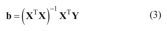
Equation 2 computes the OLS regression coefficients using a well-known formula. To decompose the regression coefficients by cases, it is sufficient to replace y (the vector of observed outcome scores) with Y = diag(y), which is a diagonal matrix that has y as the main diagonal and zeroes in all the other cells. Thus, equation 3 reveals the contribution of each case to each regression coefficient.

$$b={\left(X^{\mathrm{T}}X\right)}^{-1}{X}^{\mathrm{T}}y$$

(2)

$$b={\left(X^{\mathrm{T}}X\right)}^{-1}{X}^{\mathrm{T}}Y$$

(3)

Findings

OLS Regression Analysis

Table 2 shows the OLS models of life expectancy. These findings reproduce previously published research (Rambotti 2015), with one difference: here we use standardized variables and (thus) standardized regression coefficients. This will simplify the interpretation of case-specific contributions to the coefficients themselves. We ignore the intercept, which in standardized models is equal to zero. The results are identical to those in the original article, and their typical interpretation would emphasize the statistical significance (or lack thereof) of each regression coefficient ¹ : neither income inequality (model 1) nor poverty (model 2) is significantly associated with life expectancy; when the two variables are considered together, however, inequality becomes significant in the multiple regression (model 3). Additionally, when an interaction term between the two variables is added to the model (model 4), the interaction is significant, and the explanatory power of the model increases substantially (adjusted R² = 39 percent).

Table 2.

Standardized Coefficients and Standard Errors (in Parentheses) from Ordinary Least Squares Models of Life Expectancy.

	Model 1	Model 2	Model 3	Model 4
Income inequality	−.36		−.73*	−.68*
	(.21)		(.27)	(.24)
Poverty		.07	.56	.75**
		(.23)	(.27)	(.25)
Inequality × Poverty				−.49*
				(.20)
N	20	20	20	20
Adjusted R2	.13	.00	.22	.39
F	2.75	.08	3.80	5.22

*

p < .05 and **p < .01 (two-tailed test).

A substantive interpretation of this result, visible in Figure 1, is that higher income inequality is associated with lower life expectancy only in high-poverty countries (i.e., countries whose standardized measure of poverty is above zero). By way of contrast, income inequality is completely unrelated to life expectancy in low-poverty countries (the 12 countries in our sample whose standardized measure of poverty is below zero).

Figure 1.

Life expectancy by income inequality (all, low-poverty, and high-poverty countries). Adapted from Rambotti (2015).

A number of tests were performed to check that these models do not violate important assumptions and to check that the analysis is not sensitive to extreme outliers. For instance, because of the correlation between income inequality and poverty, it was important to evaluate collinearity in model 3. The variance inflation factor is well below the concerning threshold of 10. Visual and formal tests show that the full model presents residuals that are normally distributed and have constant variance. ² Jackknife resampling shows that standard errors are not severely biased by the possible presence of severe outliers (Quenouille 1949, 1956; Tukey 1958). All things considered, the models perform well on these tests. That being said, the characteristics of this analysis (a quantitative analysis of a small set of nonrandom observations) warrant further investigation of case-specific contributions, which is the goal of this study.

Turning Regression Inside Out

We turn our regression models inside out using the R software environment. ³ Corresponding to model 4 in Table 2, matrix X is a 20 × 3 case-by-variable matrix. Using equation 2, we obtain the same β coefficients seen in OLS model 4 above: −.68, .75, and −.49. More interestingly, if we replace y with Y = diag(y) (see equation 3), we decompose the regression coefficients into unique case-specific contributions, one per country, as shown in Table 3.

Table 3.

Ordinary Least Squares Coefficients as Sums across Cases (Model 4).

	Income Inequality	Poverty	Inequality × Poverty
AUS	.06	−.03	−.02
AUT	.00	.01	.00
BEL	.00	.00	.00
CAN	−.02	.05	−.03
CHE	.02	−.02	−.01
DEU	−.01	.01	.00
DNK	.04	.15	−.12
ESP	−.02	.06	−.03
FIN	.04	.03	−.05
FRA	.01	−.01	−.01
GBR	−.06	.03	.02
GRC	−.01	−.01	.01
IRL	−.05	−.01	.06
ISR	−.03	.08	.01
ITA	.00	.00	.00
JPN	−.45	.45	−.19
NLD	−.01	.02	.00
NOR	−.02	.00	.01
SWE	−.07	−.07	.09
USA	−.09	.01	−.24
Sum	−.68	.75	−.49

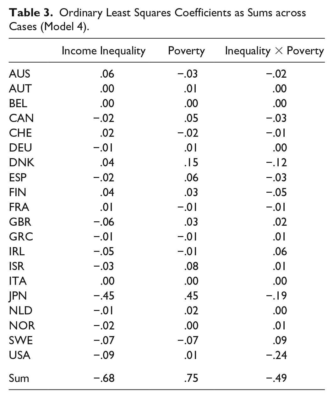
Table 3 represents a rather novel way to visualize regression analysis, which unveils a variety of stories lying underneath regression analysis. Very few precedents in the literature decompose regression coefficients by clusters of cases, in analyses of social welfare and network homophily (Melamed, Breiger, et al. 2012), and violent extremist organizations (Breiger and Melamed 2014).

We call the reader’s attention to several features of Table 3. First, notice that the last number in each column is the sum of the 20 numbers (one for each country) above it, which shows how regression coefficients are sums across case-specific contributions. In fact, −.68, .75, and −.49 are the standardized OLS coefficients for the effects of, respectively, income inequality, poverty, and the interaction of inequality and poverty on life expectancy (see model 4 in Table 2 for comparison). Second, if we focus on the last column, which shows the decomposition of the interaction coefficient, we can observe that this interaction is due largely to the contribution of a small handful of cases. Specifically, the United States, Japan, and Denmark contribute negatively (respectively, −.24, −.19, and −.12), while Sweden makes the largest positive contribution (.09). Japan and Denmark offer the highest contributions to the main effect of poverty (respectively, .45 and .15). Finally, Japan contributes most to the main effect of inequality (−.45). We propose to label these unique contributions as intensities.

Thus, 4 of 20 countries dominate the relationship in the full OLS model, which shows the largest amount of explained variation (r² = .39 for model 4 in Table 2). What happens when we look at the other models? And how do we interpret the positive and negative contributions to the regression coefficients? To answer these questions, we decompose the standardized coefficients in models 1 to 3. However, to allow a more immediate and intuitive understanding of the data, we present these country-specific intensities in visual form. ⁴ Each of the following graphs (Figures 2–5) represents a scatterplot of the countries’ life expectancy versus a predictor variable.

Figure 2.

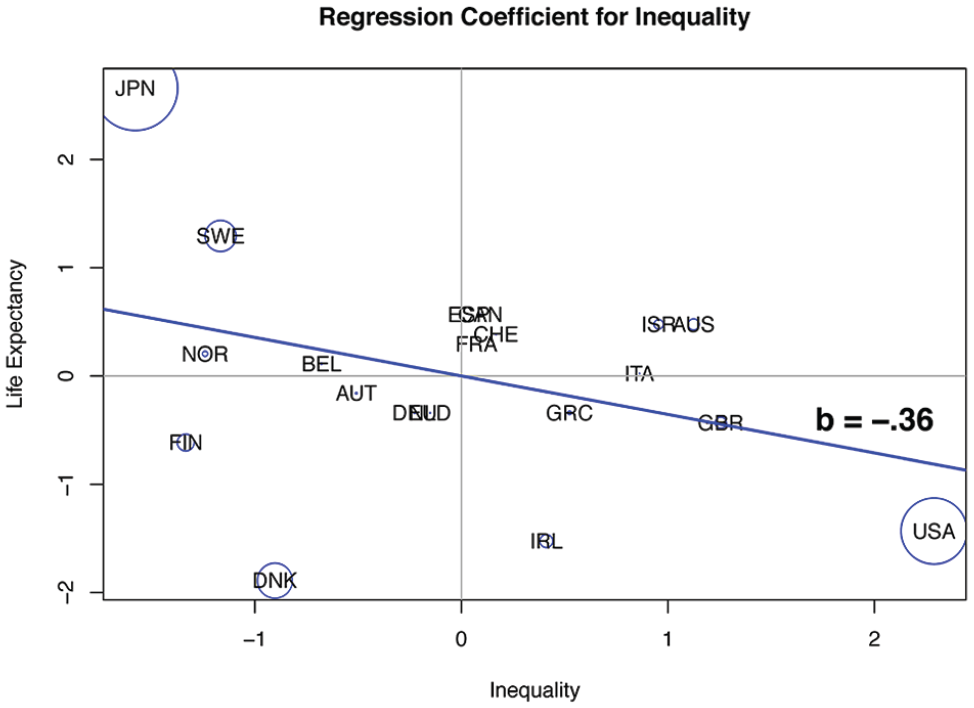
Coefficient decomposition, model 1: inequality (−.36).

Figure 3.

Coefficient decomposition, model 2: poverty (+.07).

Figure 4.

Coefficient decomposition, model 3: inequality (−.73) (A) and poverty (+.56) (B).

Figure 5.

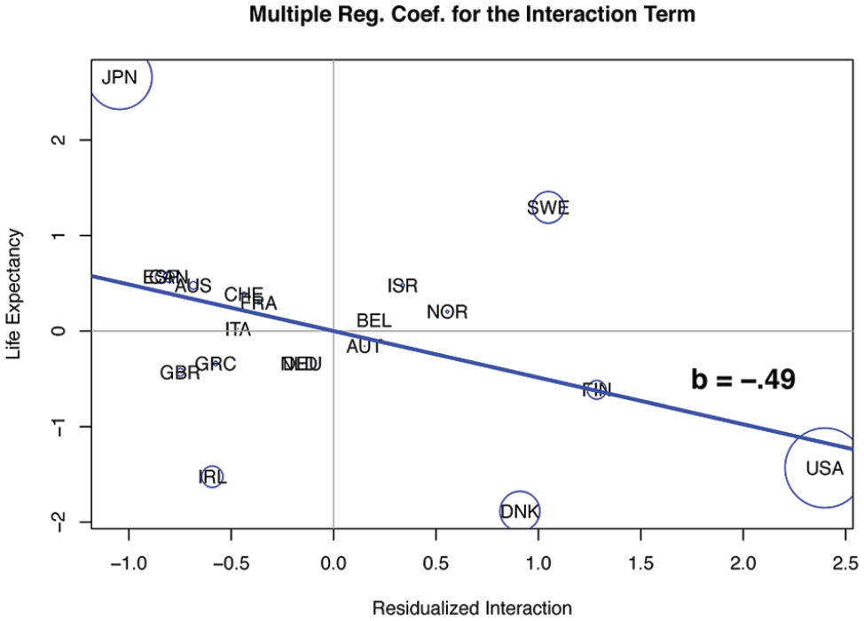
Coefficient decomposition, model 4: the interaction term (−.49).

Figure 2, for example, plots life expectancy against inequality (both variables are in standard or z-score form, with mean 0 and standard deviation 1). The overall regression coefficient is −.36. The sizes of circles in Figure 2 are proportional to countries’ contributions to the overall regression coefficient. Contributions were defined in our discussion of equation 3, and these numbers are given for selected countries in Table 4. Using Figure 2, we can illustrate what the intensities mean. Consider, for example, the nation of Sweden (SWE) in Figure 2. Sweden has less inequality than the average country we study (its score on the x axis of Figure 2 is −1.1657). Sweden’s life expectancy is above average (its score on the y axis is +1.2952). Now consider the rectangle formed by taking the coordinates of Sweden (x = −1.1657, y = +1.2952) and the coordinates of the origin (x = 0, y = 0) as the opposite corners. The area of this rectangle is the product of −1.1657 and +1.2952, which is −1.5099 (we attach the sign of the product to the area of the rectangle), which is just a constant (n − 1 = 19) times what we call Sweden’s “contribution” to the regression coefficient. This contribution is −1.5099/19 = −.0795, which is reported to two decimal places in Table 4. By the definition of the regression coefficient, the sum of the contributions equals the regression coefficient. Those contributions with positive signs are produced by countries whose x and y values are on the same side of the origin (e.g., Switzerland and Denmark in Figure 2). Conversely, contributions with negative signs result when countries are above average on one variable and below average on the other (e.g., Sweden and the United States in Figure 2).

Table 4.

Case-Specific Contributions to Coefficient Estimates.

	Denmark	Japan	Sweden	United States	Other	Total
Model 1
Inequality	.09	−.22	−.08	−.17	.03	−.36
Model 2
Poverty	.12	.06	−.07	−.16	.13	.07
Model 3
Inequality	.02	−.47	−.06	−.12	−.10	−.73
Poverty	.10	.38	−.03	−.08	.19	.56
Model 4
Inequality	.04	−.45	−.07	−.09	−.10	−.68
Poverty	.15	.45	−.07	.01	.21	.75
Interaction	−.12	−.19	.09	−.24	−.04	−.49

What do the intensities tell us about the effect of inequality on life expectancy? We see from Figure 2 that this effect is due primarily to Japan (−.2209), the United States (−.1724), Denmark (.0896), and Sweden (−.0795). The 16 remaining countries contribute little in aggregate, only a sum of .0275, to the overall regression coefficient for inequality. (Notice that these five numbers sum to the overall regression coefficient of −.36, as they must.) The directions of these intensities reflect the combination of predictor and outcome directions: Denmark has low inequality and low life expectancy (positive association); Japan and Sweden have low inequality and high life expectancy, while the United States has high inequality and low life expectancy (negative direction).

The p value for the regression coefficient (−.36) in Figure 2 is larger than .05 (see model 1 in Table 2). Inspection of Figure 2 suggests that of the four countries with the largest contribution to the overall regression coefficient, Denmark is the largest outlier with respect to the fitted line (it has the largest residual). Indeed, if this one nation is omitted, the regression coefficient across the other 19 countries becomes −.47 (p = .02 on 18 degrees of freedom).

Figure 3 shows the effect of poverty on life expectancy in model 2 (+.07, p > .05). Although the effect is positive, the largest unique contribution is negative: the intensity of United States is −.16 (high poverty, low life expectancy).

Denmark follows with an intensity of +.12, because of the combination of low poverty and low life expectancy. Sweden has the third largest intensity (−.07; low poverty and high life expectancy). Israel and Japan follow, each with an intensity of approximately +.06. Both countries have relatively high poverty (especially Israel) and high life expectancy (especially Japan).

The regression coefficient in Figure 3 has a p value larger than .05, but for a different reason than in Figure 2, in which Denmark was seen to be an outlier. In Figure 3, the five countries with the highest magnitude contributions cancel one another out: the sum of the contributions of the United States, Denmark, Sweden, Israel, and Japan is only +.0024. The other 15 countries, those with relatively lower magnitude contributions, produce a total contribution of +.0633 to the total regression coefficient of +.0657 (rounded to +.07 in model 2 of Table 2). In fact, Figure 3 illustrates an important thematic point of ours: we should be searching not for single outliers but for overall patterning of the contributions of cases, because the regression coefficient is just a sum across these case-based contributions.

Figure 4 shows the decomposed effects of inequality (in Figure 4A: coefficient = −.73, p = .016) and poverty (in Figure 4B: coefficient = +.56, p = .051) on life expectancy.

Japan and United States have the largest intensities for income inequality: −.47 (low inequality and high life expectancy) and −.12 (high inequality and low life expectancy), respectively. Japan also dominates the coefficient of poverty, with an intensity of +.38 (a relatively high poverty rate and high life expectancy), followed by Denmark (+.10). Figure 4 illustrates how our method for interpreting contributions extends to multiple regression: instead of taking inequality (for example) as the x axis, we use residuals from the regression of this variable on all other predictors. (In Figure 4A, the only other predictor is poverty.) With this stipulation, areas of rectangles are exactly proportional to case-based contributions, just as they were in Figures 2 and 3.

Finally, we turn to model 4 in Table 2, a multiple regression model including an interaction term (the coefficient for inequality is −.68, p = .014; the coefficient for poverty is +.75, p = .010; and the coefficient for the interaction is −.49, p = .031). Figure 5 shows the country contributions to the interaction. These country contributions are given in Table 3; in Figure 5 we present them in visual form.

It is clear that the interaction effect is due predominantly to the contributions of the United States, Japan, Denmark, and Sweden; the sum of their contributions in Figure 5 (see also Table 3) is −.451, out of the total regression coefficient of −.488. These four countries, then, dominate the case-specific contributions to the regression coefficients in every model that estimates the effect of income inequality, poverty—individually or simultaneously considered—and their interaction on life expectancy. These contributions are summarized in Table 4.

We noted earlier that a variety of stories may underlie regression analysis, and our findings suggest that this proposition holds true whether the coefficients achieve “statistical significance” (conventionally represented by a p value < .05) or not. Regardless of the model fit or explained variation, the story behind these associations seems to always revolve around the same four countries. Thus, one question arises: why these countries? What characterizes them?

Investigation of unusual and influential data, based on Cook’s distance and DFFITS (Belsley, Kuh, and Welsch 2004; Chen et al. 2003), shows that the United States, Japan, Denmark, and Sweden are highly influential cases. Cases can be unusual in three ways. Outliers have large residuals, which means that their outcome is poorly predicted by the regression equation (like Denmark in Figure 2). If outliers are removed from the analysis, the model fit improves. Cases have high leverage if their values on predictors are unusual; these cases can affect the estimate of regression coefficients (like the United States in Figure 5). Finally, cases have high influence, which can be thought of as a product of outlierness and leverage, if their removal drastically alter the coefficient estimates. Cook’s distance and DFFITS are measures of influence: cases above certain thresholds ⁵ are highly influential. The United States, Japan, Denmark, and Sweden have high influence on both measures (see Tables S4 and S5 in the supplemental data). It is also interesting to compare country-specific contributions with the DFBETAS, which estimate how dropping each case changes the regression coefficient (Chen et al. 2003). Across the four models, DFBETAS are highly correlated with the intensities we computed, with one major exception: the interaction term. In this case, the correlation coefficient between the intensity and the DFBETAS is .24 (p = .307). This lack of correlation is due primarily to the usual four cases: United States, Japan, Denmark, and Sweden (see Figure S2 in the supplemental data).

The relationship between intensities and DFBETAS deserves future attention, given their conceptual proximity and the empirical correlations that we often observed. The DFBETAS and our intensities are conveying related but distinct information. The DFBETAS show how much a regression coefficient changes as a result of the changes in the property space (a change in the model) that occurs when we drop an individual case. As distinct from this, our case intensities show how much each case contributes to a coefficient for a given property space (i.e., for a given model). And as we show, the intensities provide a decomposition of each regression coefficient. ⁶

Learning from Cases

What can we learn from these four influential cases? One simple way to attempt an answer is to see these countries on scatterplots that contrast life expectancy to income inequality (Figure 6) and to poverty (Figure 7).

Figure 6.

Life expectancy by income inequality: influential cases.

Figure 7.

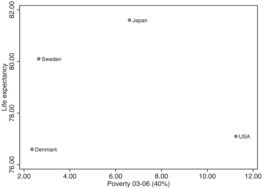
Life expectancy by poverty: influential cases.

Scholarship suggests that better health is associated with lower income inequality (Wilkinson and Pickett 2009) and (or) lower poverty (Ludwig et al. 2011, 2012). Figures 6 and 7 show that only two countries fit both theoretical expectations. The United States exhibits high levels of inequality and poverty and very low life expectancy. Conversely, Sweden shows low income inequality and poverty rates and high longevity. In sharp contrast, the cases of Denmark and Japan challenge our theoretical expectations. Denmark has very low life expectancy (lower than the United States) despite having low inequality and low poverty. Japan has high life expectancy despite having a relatively high poverty rate, which falls somewhere between the Scandinavian countries and the United States.

Denmark is part of the highly regarded Nordic model, that is, the social democratic welfare regime (Esping-Andersen 1990), which excels in a wide variety of social outcomes. In Denmark, life expectancy, however, is not one of these outcomes. Denmark’s gap in longevity is quite impressive, as it amounts to 3.5 years less than its close neighbor, Sweden. To put this into perspective, one must remember that among this set of 20 affluent countries, 1.1 years correspond to 1 standard deviation, which means that Denmark’s life expectancy is more than 3 standard deviations lower than Sweden’s. Low longevity among Danes is well documented in the health literature. A possible explanation looks at the role of wealth inequality (Nowatzki 2012), which is particularly high in Denmark. However, a number of analyses identify a more specific contribution to low longevity: the high risk for mortality for women born between the two world wars (Jacobsen et al. 2004; Jacobsen, Keiding, and Lynge 2002; Juel 2008; Juel, Bjerregaard, and Madsen 2000; Lindahl-Jacobsen et al. 2016). Interwar Danish women exhibited high rates of smoking throughout their life course and smoked more than women in any other European country (Hill 1992).

It is unclear why this is the case, but some analysts have proposed a cultural explanation based on employment: Danish women entered the labor market earlier than women in most countries, and the consequent socioeconomic autonomy might have led them to perceive smoking as a legitimate behavior (Juel et al. 2000; Nathanson 1995). Denmark has also a rather liberal tobacco policy: smoking was prohibited in restaurants, with exceptions, only in 2007 (Christensen et al. 2010). In addition to this gender-specific behavior, Danes consume more fat than any other Nordic country (Juel et al. 2000). A combination of all of these factors is likely responsible for Denmark’s low life expectancy. However, life expectancy is currently on the rise again. In fact, as interwar women (born from 1915 to 1945) are passing away, Denmark is experiencing a sharper increase in longevity than other Nordic countries (Lindahl-Jacobsen et al. 2016): such finding supports the idea that a cohort effect is truly responsible for Denmark’s observed low longevity.

In 1947, life expectancy in Japan was approximately 20 years lower than in Sweden and most Western European nations; by 1990, the Japanese were living longer than any other people (Matsuzaki 1992). Some researchers attempted to explain Japan’s longevity with sociocultural arguments, such as strong social support, an allegedly slow-paced life, ancestor worship, respect for the elderly, and overall centrality of family, especially for areas that rank high on life expectancy despite ranking low on socioeconomic indicators, such as Okinawa (Cockerham, Hattori, and Yamori 2000). The hypothesis that a close-knit fabric can protect community health and even offset typical risk factors is no stranger to social epidemiology. One prominent example is the Roseto effect (Bruhn et al. 1966; Egolf et al. 1992), which was proposed to explain why Italian American residents of Roseto, Pennsylvania, experienced low rates of heart disease despite their unhealthy lifestyle. However, Japanese longevity cannot be fully understood without considering the change in dietary habits that occurred during the twentieth century.

The Japanese diet has a number of characteristics that benefit long and healthy life expectancy. Rice is the main dish, fish intake is very high, and the ratio of animal to vegetable protein is perfectly balanced (Matsuzaki 1992). Consumption of green tea, which is extremely popular in Japan, is associated with reduced mortality from all causes and from cardiovascular disease (Kokubo et al. 2013; Kuriyama et al. 2006). Finally, the sharp decrease in salt intake after the 1950s is associated with declines in high blood pressure and strokes (Miura 2011).

Most interestingly from a sociological perspective is that this shift toward healthier lifestyles and dietary habits is the result of a precise political agenda. In fact, as the Japanese economy started growing after World War II, the health and longevity of Japanese people prospered under the “government’s strong stewardship in investing in key interventions for public health” (Ikeda et al. 2011:1094). These efforts initially reduced mortality rates for communicable diseases in children and young adults and later tackled noncommunicable diseases with initiatives such as salt reduction campaigns (Ikeda et al. 2011; Miura 2011) and cost-effective antihypertensive drugs, made available under universal health insurance coverage established in 1961 (Ikeda et al. 2011). More recently, the Japanese Ministry of Health, Labour, and Welfare and Ministry of Agriculture, Forestry, and Fisheries launched a dietary guideline known as the Japanese Food Guide Spinning Top, designed after a traditional Japanese toy (Yoshiike et al. 2007): closely following this guideline is associated with reduced mortality, for all causes and for cardiovascular disease (Kurotani et al. 2016). All in all, it is safe to conclude that Japan’s high life expectancy is truly a case of longevity by design.

Discussion

There are lessons we can learn from extremely unusual cases, and especially from cases that do not easily fit theoretical expectations. The case of Denmark demonstrates the power of cohort effects. In fact, one particular cohort, Danish interwar women, disproportionally adopted an unhealthy behavior (smoking) throughout their life course and thus altered a fundamental metric of population health (life expectancy). An approach that attempts to explain health disparities solely focusing on the highly appealing theorization of welfare regimes (Esping-Andersen 1990) is destined to fall short. Denmark shows us that every unhealthy country is unhealthy in its own way.

The case of Japan demonstrates the power of government initiative and foresight. Over several decades, the Japanese government introduced universal health coverage and cost-effective treatments and promoted healthy lifestyle and dietary habits. These measures proved remarkably successful in reducing mortality and increasing longevity, even in the presence of issues such as high relative poverty, rising unemployment, diffuse overwork, karoshi (death from overwork), suicide, and stigmatized mental health (Chen, Choi, and Sawada 2009; Ikeda et al. 2011; Kondo and Oh 2010; Motohashi 2012; Ozawa-de Silva 2008). What Japan actually suggests is that healthy countries are not all alike.

Although it is important to learn lessons from unique cases, it would be a mistake to extrapolate some of their characteristics and use them “as a means of drawing generalizable inferences” (Kenworthy 2007:349). For instance, one could look at Japan and argue that it provides evidence in favor of the IIH. After all, Japan has high longevity, low inequality, and high poverty. However, there is disagreement on the actual level of inequality in Japan. The Organisation for Economic Co-operation and Development (OECD), for instance, contends that considering Japan as the most equal among industrialized countries “depends on the use of an alternative official data source (NSFIE) that appears as less suited for assessing income inequality and poverty” (OECD 2012:228). The OECD’s conclusion is supported by data available from other sources. The most comprehensive data set on this topic is arguably the World Wealth and Income Database.

Using the Wealth and Income Database’s share of the top 10 percent income earners, Figure 8 shows the historical trends of income inequality in Denmark, Japan, Sweden, and the United States. This picture suggests that Japan is actually rather unequal overall, more unequal than Denmark and Sweden, and facing rising inequality. More important, if Japan’s inequality increased while Japan’s longevity increased, the IIH loses support. Inconsistent time trends of this type have been long observed in the literature, with researchers (Lynch and Davey Smith 2003) urging the use of longitudinal methodology. ⁷ However, even if Japan were indeed equal, a researcher who aims to propose a causal link between income equality and longevity should try to explain why this link disappears (see Figure 9; compare our discussion of Figure 2) when the four influential countries are removed.

Figure 8.

Top 10 percent income share: historical trend.

Figure 9.

Life expectancy by income inequality: noninfluential cases.

Conclusion

In this study we use a novel methodology (Breiger et al. 2011; Breiger and Melamed 2014; Melamed, Breiger, et al. 2012; Melamed, Schoon, et al. 2012), which turns regression models inside out. With this approach, we are able to decompose regression coefficients into country-specific contributions, which show the intensity of each case on estimated effects, and we are able to uncover multiple dynamics underlying regression analysis. We applied this methodology to a comparative study of health and inequality. We showed that the same logic of case contribution underlies the relationship, regardless of model fit. While assessing what matters more for life expectancy—inequality, poverty, or their interaction—one might fail to notice that the same four highly influential cases (the United States, Sweden, Denmark, and Japan) dominate all models. Every macro-comparative analysis of the social determinants of population health is destined to miss the mark unless a logic of case contribution is uncovered. By turning the regression “inside out,” we bring the logic of case contribution to the center of the analysis.

This study presents limitations typical of macro-comparative cross-sectional analysis. Unobserved heterogeneity between countries might bias the findings. Although our decomposition of our poverty measure into county-specific contributions is sensible, the decomposition of the inequality estimate is still likely to hide potential differential inequality dynamics. Along those lines, Liao (forthcoming) develops and applies methods for identifying case-specific contributions to social inequality measures that reveal hidden dynamics. This is of great substantive importance, but it does not lessen the usefulness of the method proposed here.

Cross-sectional data prevent us from observing time trends. To better assess the relationship between income inequality and health, it is more appropriate to choose a methodology that overcomes these limits. One strategy is to focus on subnational variation over time. Focusing on variation within a country is advantageous also because it enables comparison of specific policies meant to mitigate social inequalities or health issues. The United States represents a case of particular interest, insofar as it is “somewhat exceptional in that it is the country where income inequality is the most consistently linked to population health” (Lynch et al. 2004:81). Whether this finding is robust to different model specifications, which incorporate underused indicators of income inequality and health and estimate random versus fixed regional effects, is still to be determined. However, it is important to notice that such models are not necessarily immune to the logic of case contribution, which future research should consider by turning longitudinal regressions “inside out.” Finally, a fundamental limitation is represented by the macro nature of our data. If we applied this methodology to individual-level data, the very meaning of what a case is would be different, insofar as it would not be possible to identity a few substantial cases (i.e., countries) to analyze in depth. However, this does not mean that this methodology is exclusively limited to macro data. As noted earlier (see discussion of Figure 3), the ultimate goal should not be to simply pinpoint single outliers but to uncover the overall patterning of contributions across all the cases, including clusters of individuals. This is consistent with a previous application of the methodology, which used General Social Survey data to show how clustering of cases is dual to interactions of variables (Melamed, Breiger, et al. 2012). Future research should attempt to turn individual-level regressions “inside out” to inductively detect clustering of cases, which may provide insights to advance sociological theory.

Supplemental Material

extreme_and_inconsistent_code_including_data – Supplemental material for Extreme and Inconsistent: A Case-Oriented Regression Analysis of Health, Inequality, and Poverty

Supplemental material, extreme_and_inconsistent_code_including_data for Extreme and Inconsistent: A Case-Oriented Regression Analysis of Health, Inequality, and Poverty by Simone Rambotti and Ronald L. Breiger in Socius

Supplemental Material

extreme_and_inconsistent_supplemental_material – Supplemental material for Extreme and Inconsistent: A Case-Oriented Regression Analysis of Health, Inequality, and Poverty

Supplemental material, extreme_and_inconsistent_supplemental_material for Extreme and Inconsistent: A Case-Oriented Regression Analysis of Health, Inequality, and Poverty by Simone Rambotti and Ronald L. Breiger in Socius