Sage Journals: Discover world-class research

Abstract

The Fragile Families Challenge is a scientific mass collaboration designed to measure and understand the predictability of life trajectories. Participants in the Challenge created predictive models of six life outcomes using data from the Fragile Families and Child Wellbeing Study, a high-quality birth cohort study. This Special Collection includes 12 articles describing participants’ approaches to predicting these six outcomes as well as 3 articles describing methodological and procedural insights from running the Challenge. This introduction will help readers interpret the individual articles and help researchers interested in running future projects similar to the Fragile Families Challenge.

Keywords

life course prediction mass collaboration common task method machine learning

Introduction

Social scientists studying the life course have described social patterns, theorized factors that shape outcomes, and estimated the effects of specific interventions. However, it is unclear how much the knowledge developed from this prior research enables researchers and policymakers to accurately predict life outcomes. Although social scientists have generally focused on questions about explanation rather than questions about prediction (Breiman 2001; Hofman, Sharma, and Watts 2017; Shmueli 2010; Yarkoni and Westfall 2017), questions about prediction are important for three reasons.

First, there is growing interest in using predictive models to target assistance to children and families at risk (Kleinberg et al. 2015). For example, policymakers in Allegheny County, Pennsylvania, are currently using predictive models to assist case workers in deciding whether a maltreatment referral about a child is of sufficient concern to warrant an in-person investigation (Chouldechova et al. 2018; Eubanks 2018). Although using predictive models in policy settings raises important questions about data collection (Barocas and Selbst 2016; Lakkaraju et al. 2017), fairness (Courtland 2018), and causal inference (Athey 2018), the use of predictive models in policy settings is nevertheless likely to accelerate. Basic scientific knowledge about the predictability of life outcomes can serve as a guide for future policymaking around these models.

Second, the predictability of a person’s life outcomes is a measure of social rigidity (Blau and Duncan 1967): the degree to which future outcomes can be predicted by family characteristics or past experience. Measures of rigidity, such as the relationship between a father’s and son’s occupation, have been the subject of extensive sociological research (Torche 2015). Although this research has tended to focus on statistical association, these questions can also be framed in terms of prediction: Given certain background information about a person, how well can we predict what will happen to them at a later time?

Third, efforts to improve predictive performance can spark developments in theory, methods, and data collection, even in settings where prediction is not of direct scientific interest. The finding that some important life outcomes are not very predictable from the kinds of data that social scientists normally collect could lead to numerous improvements. For example, researchers could theorize about social processes not currently being considered and develop new methods to better utilize available data. Any of these developments should be welcomed, even by researchers who have little interest in prediction.

To measure and understand the predictability of life trajectories, we organized a scientific mass collaboration called the Fragile Families Challenge. Our mass collaboration used a research design from machine learning that is ideally suited to measuring predictability: the common task method (Donoho 2017). In projects using the common task method, all participants use the same data to predict the same outcomes. Further, these predictions are all evaluated in the same way: predictive accuracy measured with held-out data (data that were not available to participants when they were making predictions). The standardization created by the common task method ensures that many different approaches can be compared fairly, and the use of held-out data limits the amount that reported levels of predictive accuracy can be inflated by overfitting. Because of these attractive characteristics, the common task method is widely used by research communities focused on predictive accuracy, and Donoho (2017) called it the “secret sauce” of machine learning.

The common task method is typically defined by three elements: a common data set, a common task, and a common evaluation metric. Each of these elements will be described in detail later and are summarized here. In the Fragile Families Challenge, the common data set was a specially constructed version of the Fragile Families and Child Wellbeing Study, a high-quality birth cohort study. This ongoing study was designed to understand the dynamics of families formed by unmarried parents and the lives of children born into these families. It collects rich longitudinal data about thousands of families who gave birth to a child in large U.S. cities around the year 2000. These data—which have been used in more than 750 published journal articles¹—were collected in six waves (child birth and ages 1, 3, 5, 9, and 15 years) and include many factors that researchers think are important predictors of child well-being. The common task was to use these data to predict six outcomes variables measured at child age 15: (1) child grade point average (GPA), (2) child grit, (3) household eviction, (4) household material hardship, (5) caregiver layoff, and (6) caregiver participation in job training. Finally, the common evaluation metric was mean squared error (MSE) in held-out data.

We received applications from 457 researchers from a variety of fields who wanted to participate in the Challenge, and we shared data with 437 of them. These researchers often worked in teams, and we received valid submissions from 160 teams.

This Socius Special Collection—along with the Salganik et al. (2020)—reports the results of the predictive modeling stage of the Fragile Families Challenge. The Special Collection includes 12 articles describing participants’ approaches to the Challenge as well as 3 articles describing what we learned from running the Challenge. There is also a comment on one of the articles.

This introduction has three goals. First, it provides background about the Challenge, which will help readers understand and interpret the individual articles. Second, it highlights themes that run through the articles. Third, it shares ideas that may be helpful to researchers who wish to design or participate in a similar project. The remainder of this introduction has three parts. First, we describe the Fragile Families Challenge, focusing on the data, prediction task, and evaluation metric. Next, we provide an overview of approaches used in the Special Collection. Finally, we provide some performance benchmarks that can help readers interpret the predictive performance values reported in the papers. Supplemental Material includes the call for papers for this Special Collection and information about the review process. Some of the descriptions of the Fragile Families Challenge also appear in the Salganik et al. (2020) and are repeated here for clarity.

The Fragile Families Challenge

Data

The data used in the Fragile Families Challenge came from the Fragile Families and Child Wellbeing Study (FFCWS). The FFCWS began with a multistage, stratified random sample of hospital births between 1998 and 2000 in large U.S. cities (more than 200,000 residents), with a 3:1 oversample of births to nonmarried parents (Reichman et al. 2001). Once a family agreed to participate in the study, data were collected when the child was born and then at approximately child ages 1, 3, 5, 9, and 15 years. Data collection included members of the biological family (e.g., mother, father, child) as well as others (e.g., teachers; Figure 1). FFCWS collects information about numerous factors that researchers think are important predictors of child well-being, including demographic, family, and neighborhood characteristics; parents’ health and employment status; parenting behavior; children’s cognitive test scores and behaviors; and the physical home environment (Table 1). In addition to data collected directly from respondents, the FFCWS data also include survey paradata (e.g., sampling weights) and constructed variables derived from the originally collected data. For example, during the in-home visit when the child was three years old, the child was given the Peabody Picture Vocabulary Test (PPVT), a standardized test to measure the vocabulary of children (Dunn and Dunn 2007). In addition to providing responses to each question in the PPVT, the FFCWS data also include a constructed PPVT score.

Figure 1.

Data collection modules in the Fragile Families and Child Wellbeing Study that were used in the Fragile Families Challenge. The background data set used in the Fragile Families Challenge used data collected at birth and years 1, 3, 5, and 9. The six outcome variables were chosen from all the variables that were collected at child age 15.

Table 1.

Information Collected in the Fragile Families and Child Wellbeing Study between Child Birth and Age Nine.

Data Module	Child Age	Domains
Mother	Birth	(A) Child health and development, (B) father-mother relationships, (C) fatherhood, (D) marriage attitudes, (E) relationship with extended kin, (F) environmental factors and government programs, (G) health and health behavior, (H) demographic characteristics, (I) education and employment, (J) income
Father	Birth	(A) Child health and development, (B) father-mother relationships, (C) fatherhood, (D) marriage attitudes, (E) relationship with extended kin, (F) environmental factors and government programs, (G) health and health behavior, (H) demographic characteristics, (I) education and employment, (J) work activities, (K) income
Mother	1	(A) Family characteristics, (B) child well-being and mothering, (C) father-child relationship, (D) mother’s relationship with father, (E) current partner, (F) demographics, (G) mother’s family background and support, (H) environment and programs, (J) health and health behavior, (K) education and employment, (L) income
Father	1	(A) Family characteristics, (B) child well-being and fathering, (C) mother-child relationship, (D) father’s relationship with mother, (E) current partner, (F) demographics, (G) father’s family background and support, (H) environment and programs, (J) health and health behavior, (K) education and employment, (L) income
Mother	3	(A) Family characteristics, (B) child well-being and mothering, (C) father-child relationship, (D) mother’s relationship with father, (E) current partner, (F) demographics, (H) mother’s family background and support, (I) environment and programs, (J) health and health behavior, (R) religion, (K) education and employment, (L) income
Father	3	(A) Family characteristics, (B) child well-being and fathering, (C) mother-child relationship, (D) father’s relationship with mother, (E) current partner, (F) demographics, (H) father’s family background and support, (I) environment and programs, (J) health and health behavior, (R) religion, (K) education and employment, (L) income
Primary caregiver and in-home observation	3	(A) Health and accidents, (B) family routines, (C) home toy and activity items, (D) nutrition, (E) food expenditures, (F) housing/building characteristics, (G) parental stress, (H) parental mastery, (J) discipline, (K) informal social control and social cohesion and trust, (L) exposure to violence, (M) child’s behavior problems, (P) observation checklist, (Q) common areas, (R) interior of house or apartment, (S) child’s appearance, (T) home scale, (U) child emotion and cooperation, (V) ending
In-home activities with child and mother	3	(A) Height and weight, (B) Child’s Peabody Picture Vocabulary Test or TVIP, (C) Walk-A-Line, (D) Q-Sort, (E) Mothers Peabody Picture Vocabulary Test or TVIP, (F) child care/employment history calendar
Child care provider survey (for center-based care)	3	(A) Care provided at the center, (B) care provided for focus child, (C) care provided for focus child, (E) teacher-parent relationship, (F) teacher beliefs, (G) about the child care teacher
Child care center observations	3	No clear section headings but contents include: space and furnishings, personal care routines, language-reasoning, activities, interaction, program structure, parents and staff
Family care provider survey (for family-based care)	3	(A) Care provided, (B) child care routine and program, (D) provider-parent relationship, (E) child care provider beliefs, (F) about the child care provider
Family care provider observations	3	No clear section headings but contents include: space and furnishings for care and learning, basic care, language and reasoning, learning activities, social development
Child care study postobservation form	3	(A) Observation checklist, (B) common areas, (C) interior of building, (D) home scale, (E) postvisit rating by interviewer
Mother	5	(A) Family characteristics, (B) child well-being and mothering, (C) father-child relationship, (D) mother’s relationship with father (for mothers who are or were in a relationship) (E) current partner, (F) demographics, (H) mother’s family background and support, (I) environment and programs, (J) health and health behavior, (R) religion, (K) education and employment, (L) income
Father	5	(A) Family characteristics, (B) child well-being and fathering, (C) mother-child relationship, (D) father’s relationship with mother (for fathers who are or were in a relationship), (E) current partner, (F) demographics, (H) father’s family background and support, (I) environment and programs, (J) health and health behavior, (R) religion, (K) education and employment, (L) income
Primary caregiver and in-home observation	5	(A) Health and accidents, (B) family routines, (C) home toy and activity items, (D) nutrition, (E) housing/building characteristics, (F) parental stress and mastery, (G) discipline, (H) exposure to violence, (J) Child Protective Services contact, (K) food expenditures, (L) child’s behavior, (N) activities, (P) observation checklist, (Q) common areas, (R) interior of house or apartment, (S) child’s appearance, (T) home scale, (U) child emotion and cooperation, (V) ending
In-home activities with child and mother	5	(A) Weight/height, (B) Peabody Picture Vocabulary Test with child, (C) Woodcock-Johnson Letter-Word activity with child, (D) attention sustained task, (E) child care employment history calendar, (F) five-minute speech sample, (G) Peabody Picture Vocabulary Test with mother
Teacher	5	(A) Information specific to the participating child, (B) academic skills specific to the participating child, (C) classroom behavior and social skills specific to the participating child, (D) classroom characteristics, (E) class resources and activities, (F) school climate and environment, (G) general information about teacher
Mother	9	(A) Core mother interview: family characteristics, household roster, marital, and fertility history; (B) bio father contributions and resources; (C) mother’s relationship with father; (D) current partner; (E) mother’s family background and support; (F) environment and programs; (G) health and health behavior; (H) religion; (I) education and employment; (J) income; (K) secondary caregiver
Father	9	(A) Core father interview: family characteristics, household roster, marital, and fertility history; (B) bio mother and bio father contributions and resources; (C) father’s relationship with mother; (D) current partner; (E) father’s family background and support; (F) environment and programs; (G) health and health behavior; (H) religion; (I) education and employment; (J) income; (K) secondary caregiver
Primary caregiver	9	(A) Introduction to nonparental caregiver survey; (B) mother-child relationship; (C) father-child relationship; (D) demographics; (E) income, education, and employment; (F) health and well-being; (G) environment; (H) health and accidents; (I) family routines and home life; (J) nutrition; (K) parental stress and mastery; (L) child’s education; (M) child’s neighborhood
Interviewer observation	9	(A) Observation checklist, (B) common areas, (C) interior of house or apartment, (D) child’s appearance, (E) home scale, (F) child emotion and cooperation, (G) ending
		(A) Parental supervision and relationship, (B) parental discipline, (C) sibling relationships, (D) routines, (E) school, (F) early delinquency, (G) task completion and behavior, (H) health and safety, (I) closing
In-home activities with child and primary caregiver	9	No clear section headings but activities include: consent, child assessment (PPVT, Digit Span, Woodcock-Johnson Tests 9 and 10), primary caregiver self-administered questionnaire, health measures, saliva sample, biological mother weight, child weigh/height, primary caregiver open-ended responses
Teacher	9	(A) General information, (B) classroom behavior and social skills specific to the participating child, (C) information specific to the participating child, (D) parent/guardian involvement, (E) classroom characteristics, (F) school climate and environment, (G) general information about teacher

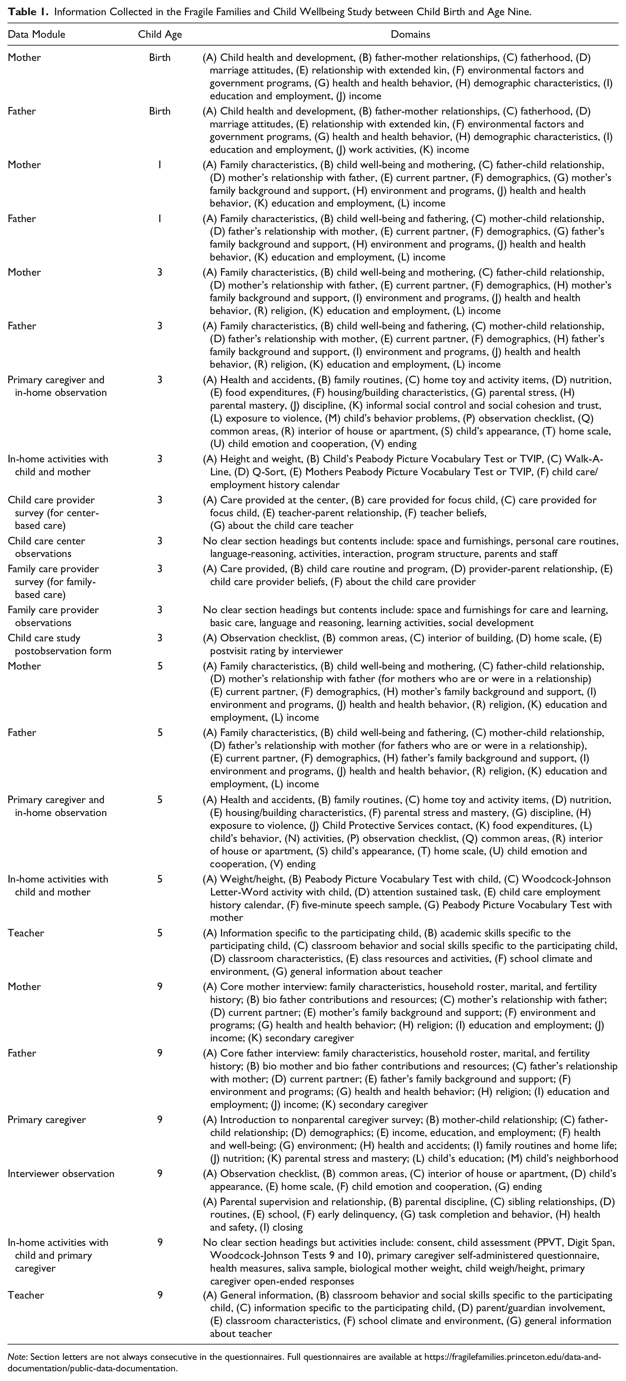
Note: Section letters are not always consecutive in the questionnaires. Full questionnaires are available at https://fragilefamilies.princeton.edu/data-and-documentation/public-data-documentation.

The common data in the Fragile Families Challenge was a specially constructed version of the FFCWS data that was split into four data sets: background, training, leaderboard, and holdout (Figure 2). The background data included thousands of variables that were collected about the family in the first nine years of the child’s life. The training, leaderboard, and holdout data included the six outcome variables collected at child age 15.

Figure 2.

Data sets in the Fragile Families Challenge. The background data were collected between child birth and child age nine. The six outcome variables, which were collected at child age 15, were split into three sets: training (four of eight observations), leaderboard (one of eight observations), and holdout (three of eight observations). Participants in the Challenge used the background and training data to predict outcomes. The accuracy of predictions in the leaderboard data set was available during the Challenge, and the accuracy of predictions in the holdout data set was available only at the end of the Challenge.

To construct the background data set, we began with the basic FFCWS files, which are available to researchers through an application process. Then we took three steps. First, we combined many data files containing information on the focal child into a single file. Second, we dropped observations that were obtained in 2 out of the 20 cities of birth because these were pilot cities where some questions were asked differently or not at all. Third, we made changes to the data to promote the privacy of respondents and reduce the risk of harm in the event of reidentification: We redacted some variables, edited some variables, and added noise to other variables (Lundberg 2019). For example, because of our privacy and ethics audit, we decided that the background data set would not contain genetic and geographic information even though this information has been collected in the FFCWS (Lundberg et al. 2019). Ultimately, the background data set had information about 4,242 families and 12,942 variables plus an ID number for each family.

The background data set contained approximately 55 million possible entries (4,242 × 12,942). However, about 73 percent of possible entries did not have a value (Figure 3a). Many of the papers in the Special Collection spend time addressing these missing values. There are several different reasons that a possible data entry might not have a value (Figure 3b), not all of which map cleanly onto how many social scientists think about missing data. We highlight four main reasons. First, some entries were missing because participants did not participate in one of the follow-up interviews (about 17 percent of entries). Second, some entries were missing because respondents refused or were unable to answer a specific question (less than 1 percent of entries). Third, some entries were missing because our privacy and ethics audit redacted certain variables (Lundberg et al. 2019; about 6 percent of entries). Finally, some entries were missing because of skip patterns in the survey (25 percent of entries). For example, when the child was nine years old, the father was asked to describe his current living situation (Figure 4). There were 10 possible responses (e.g., rent a home, own a home, homeless), and the subsequent questions depended on the response given. These skip patterns were an intentional part of the questionnaire design. Two papers in the Special Collection make a special effort to deal with these intentional skips (Carnegie and Wu 2019; Goode, Datta, and Ramakrishnan 2019).

Figure 3.

Missing entries in the Fragile Families Challenge background data set. The background data set had 4,242 rows and 12,942 columns (plus an ID number). Of the approximately 55 million distinct data entries, about 73 percent were missing. There were many types of missing values.

Figure 4.

Example skip pattern in the Fragile Families and Child Wellbeing Study. Depending on the answers to this question, which was asked to the father when the child was nine years old, the respondent would be asked different follow-up questions. These skip patterns caused some of the missing entries in the background data set.

The other three data sets—training, leaderboard, and holdout—consisted of the six outcome variables that were collected when the child was 15 years old. During the Challenge, participants had full access to the training data, partial access to the leaderboard data, and no access to the holdout data. Participants used the background data and training data to learn (estimate) a statistical or machine learning model (e.g., the coefficients of ordinary least squares regression). Participants then used these models to make predictions for all observations. During the Challenge, participants could upload their submissions—which included their predictions, their code, and a narrative explanation of their approach—to our submission platform.² Our platform then calculated the mean squared prediction error in the leaderboard data and showed this score on a leaderboard that was visible to all participants. Finally, at the end of the Challenge, we calculated the mean squared error of the predictions in the holdout data.

When deciding the relative sizes of the training, leaderboard, and holdout data sets, we balanced a tension between having the largest possible training data set (to enable more accurate predictions) and the largest possible holdout data set (to enable more accurate estimates of the predictive performance). Ultimately, we allocated four of eight of observations to the training data set, one of eight to the leaderboard data set, and three of eight to the holdout data set. This allocation was somewhat arbitrary but similar to that used in other projects using the common task method. Given these relative sizes, we allocated data by systematic sampling to make them as similar as possible (Särndal, Swensson, and Wretman 2003). We first sorted all observations by city of birth, parents’ relationship status at the birth, mother’s race, whether at least one outcome was nonmissing, and then the outcomes in the following order: eviction, layoff, job training, GPA, grit, and material hardship. In the sorted data, we grouped observations into sets of eight sequential observations. Then, we randomly assigned four, one, and three of the observations to the training, leaderboard, and holdout data sets.

Table 2 summarizes the number of nonmissing outcome cases in each of the training, leaderboard, and holdout data sets. Cases with missing outcomes were not used when measuring the mean squared prediction error in the holdout data. In the leaderboard data set only, we imputed missing values on the outcome variables by taking a random sample (with replacement) from the distribution of observed outcomes. Because these random draws are unpredictable by construction, this gave us a tool to assess whether respondents were overfitting to the leaderboard set by submitting numerous queries and updating their models accordingly.³

Table 2.

Number of Nonmissing Cases for Each Outcome in the Training, Leaderboard, and Holdout Data Sets.

Outcome	Training	Leaderboard	Holdout
Grade point average	1,165	304	886
Grit	1,418	362	1,075
Material hardship	1,459	375	1,099
Eviction	1,459	376	1,103
Layoff	1,277	327	994
Job training	1,461	376	1,104
Total possible	2,121	530	1,591

Prediction Task

The common task in the Challenge was to use the background and training data to predict six outcome variables measured at child age 15: (1) child GPA, (2) child grit, (3) household eviction, (4) household material hardship, (5) caregiver layoff, and (6) caregiver participation in job training. At the time of the Challenge, these data were available only to survey administrators and a very small set of researchers who were not allowed to participate in the Challenge. Participants in the Challenge could focus on predicting as many of these outcomes as they wished. Table 3 summarizes the outcomes variables of interest in each paper in the Special Collection.

Table 3.

Outcomes That Are the Focus of the Authors’ Attention.

Paper	Outcome(s)
Ahearn and Brand	Layoff
Altschul	All
Carnegie and Wu	All
Compton	All
Davidson	GPA
Filippova et al.	All
Goode, Datta, and Ramakrishnan	All
McKay	All
Raes	GPA
Rigobon et al.	All
Roberts	GPA
Stanescu, Wang, and Yamauchi	All

Note: “All” indicates that the authors focused on all six outcomes: grade point average (GPA), grit, material hardship, eviction, layoff, and job training.

The choice of the six outcome variables from the approximately 1,500 variables measured at age 15 was a key design decision. We chose outcome variables for which good predictions would be useful for subsequent substantive research. For the continuous outcomes, we planned to study families that were doing much better than predicted and much worse than predicted, so we wanted outcome variables that were important to social scientists and policy makers, poorly understood, and measured well. For the binary outcomes, we planned to consider these variables as treatments and measure their effects on a new set of outcomes later in the life course (e.g., college enrollment), so we wanted variables that were important to social scientist and policymakers, common enough to be meaningful, and conducive to clean causal claims.⁴ Methodologically, we wanted a variety of variable types—such as continuous and binary or about the child, household, or primary caregiver—so that we could study the relationship between the type of outcome, its overall predictability, and the best methods for predicting it. The appropriate number and type of outcome variable(s) for future mass collaborations is an open question.

The exact operationalization of these six outcome variables differs across the scientific literature. Table 4 describes our approach. For two outcomes in particular—eviction and grit—we emphasize differences between how the FFCWS measured these outcomes and how they are measured in other research. The measure of eviction in the FFCWS includes eviction for nonpayment of rent or mortgage, regardless of whether a court ordered the eviction or a landlord carried it out informally (Desmond and Kimbro 2015; Lundberg and Donnelly 2019). Other research focuses on formal court-ordered evictions for any reason (Desmond et al. 2018). The FFCWS measurement of grit is different from the measure proposed in Duckworth et al. (2007), whose original grit scale consists of six items related to consistency of interest and six items related to perseverance of effort. The FFCWS scale is shorter (four items) and was designed with adolescent school outcomes in mind. Two items (“I finish whatever I begin”; “I am a hard worker”) are exactly as in the original scale for perseverance of effort. One item on the FFCWS scale (“Once I make a plan to get something done, I stick to it”) is a simplified version of one of the original items about consistency of interests (“I have difficulty maintaining my focus on projects that take more than a few months to complete”). Likewise, the FFCWS scale includes an item focused on schoolwork (“I keep at my schoolwork until I am done with it”), which is a more targeted version of an item from the original perseverance scale (“I am diligent”). A final difference is that Duckworth et al. (2007) proposed a scale with five answer choices (not at all like me to very much like me), whereas the FFCWS scale involves four choices (strongly disagree to strongly agree).

Table 4.

Outcome Variables Measured at Child Age 15.

Age 15 Outcome	Age 9 Questions	Response Values	Reporter	How Aggregated
Grade point average	At the most recent grading period, what was your grade in 1. English or language arts? 2. Math? 3. History or social studies? 4. Science?	1. A2. B3. C4. D or lower	Child	Reverse-coded and averaged. Marked NA if any item missing due to no grade, pass/fail, refusal, don’t know, or not interviewed.
Grit	Thinking about how you have behaved or felt during the past four weeks, please tell me whether you strongly agree, somewhat agree, somewhat disagree, or strongly disagree with the following statements. 1. I keep at my schoolwork until I am done with it. 2. Once I make a plan to get something done, I stick to it. 3. I finish whatever I begin. 4. I am a hard worker.	1. Strongly agree2. Somewhat agree3. Somewhat disagree4. Strongly disagree	Child	Reverse-coded and averaged. Marked NA if any item missing due to refusal, don’t know, or not interviewed.
Material hardship	We are also interested in some of the problems families have making ends meet. In the past twelve months, did you do any of the following because there wasn’t enough money? 1. Did you receive free food or meals? 2. Were you ever hungry, but didn’t eat because you couldn’t afford enough food? 3. Did you ever not pay the full amount of rent or mortgage payments? 4. Were you evicted from your home or apartment for not paying the rent or mortgage? 5. Did you not pay the full amount of gas, oil, or electricity bill 6. Was your gas or electric services ever turned off, or the heating oil company did not deliver oil, because there wasn’t enough money to pay the bills? 7. Did you borrow money from friends or family to help pay bills? 8. Did you move in with other people even for a little while because of financial problems? 9. Did you stay at a shelter, in an abandoned building, an automobile, or any other place not meant for regular housing, even for one night?10. Was there anyone in your household who needed to see a doctor or go to the hospital but couldn’t go because of the cost?11. Was your telephone service (mobile or land line) cancelled or disconnected by the telephone company because there wasn’t enough money to pay the bill?	1. Event did not occur2. Event occurred	Child’s primary caregiver	Averaged. Marked NA if any response missing due to refusal, don’t know, or not interviewed.
Eviction	1. In the past twelve months, were you evicted from your home or apartment for not paying the rent or mortgage? 2. (If no above:) Since [month and year of interview at approximately child age 9], were you evicted from your home or apartment for not paying the rent or mortgage?	1. No2. Yes	Child’s primary caregiver	If no to both questions, 0. If yes to either question, 1. Marked NA if missing due to refusal, don’t know, or not interviewed.
Layoff	Since [month and year of interview at approximately child age 9], have you been laid off from your employer for any time?	1. No2. Yes	Child’s primary caregiver	Marked NA if missing due to refusal, don’t know, or not interviewed.
Job training	Since [month and year of interview at approximately child age 9], have you been laid off from your employer for any time?	1. No2. Yes	Child’s primary caregiver	Marked NA if missing due to refusal, don’t know, or not interviewed.

Evaluation Metric

There are many potential metrics by which to evaluate predictive performance, and these different metrics can lead to different conclusions (Hofman et al. 2017). When choosing the evaluation metric for the Fragile Families Challenge, we wanted one that was: (1) familiar to participants, (2) applicable to both binary and continuous outcomes, and (3) aligned with the scientific objectives of the next stage of the Fragile Families Challenge.

We decided that MSE was best suited to this task:

{MSE}_{Holdout} = \frac{1}{n_{Holdout}} \sum_{i \in Holdout} {(y_{i} - {\hat{y}}_{i})}^{2},

(1)

where $y_{i}$ is the outcome for person $i$ (e.g., GPA), ${\hat{y}}_{i}$ is the predicted outcome for person $i$ , and $n_{Holdout}$ is the number of people in the holdout set, excluding missing cases.

We selected MSE for three reasons. First, MSE is a well-known metric that those working with predictive models would have encountered previously. Second, mean squared error is a very common metric regardless of whether the outcome is binary (Brier 1950) or continuous (e.g., ordinary least squared regression minimizes squared error). Third, one goal of the predictive modeling stage of the Fragile Families Challenge was to identify families with outcomes very far from their expected values given the predictors. The optimal submission to minimize MSE would predict the expected values for all observations if this quantity were known. Mean squared error therefore aligned with our substantive goals.

To increase interpretability and increase comparability across outcomes, some papers present results in terms of $R_{Holdout}^{2}$ , which compares the accuracy of a set of predictions to the accuracy of prediction of the mean of the training data, which could be considered an extremely simple baseline prediction.

R_{Holdout}^{2} = 1 - \frac{\sum_{i \in Holdout} {(y_{i} - {\hat{y}}_{i})}^{2}}{\sum_{i \in Holdout} {(y_{i} - {\bar{y}}_{Training})}^{2}},

(2)

where ${\bar{y}}_{Training}$ is the mean of the training data.⁵

Overview of Approaches

Although the papers in this Special Collection may appear different, they share a similar structure. Most of them describe approaches to the Challenge that involved four steps: data preparation, variable selection, statistical learning, and model interpretation. Data preparation encompasses the procedures by which the authors converted the data and survey documentation into a format suitable for analysis (Table 5). Variable selection captures how authors chose a subset of variables to use when predicting the outcome (Table 6). Statistical learning includes all steps by which the authors learn (estimate) a function linking those variables to the outcome. We choose the term statistical learning because we include approaches common in statistics (e.g., generalized linear model) as well as approaches common in machine learning (e.g., random forest; Table 7). Finally, model interpretation—a step not required for the Challenge but carried out by many authors nonetheless—is our term for authors’ efforts to summarize the resulting model (Table 8). By placing the authors’ contributions within the framework of these four steps, we are able to highlight the general themes that emerge in varying forms across papers. To bound this section, we only describe approaches that appear in more than one paper of this Special Collection, and we do not describe each approach in detail. Friedman, Hastic, and Tibishirani (2001) and Efron and Hastie (2016) provide more detailed introductions to many of the approaches used in the Challenge, and Mullainathan and Spiess (2017), Athey (2018), and Molina and Garip (2019) provide more detailed introductions to how these methods are used in the social sciences.

Table 5.

Data Preparation Approaches.

	Inferring Categorical Features	Imputing Missing Data				Creating Synthetic Features
Author	Inferring Categorical Features	Mean, Median, Mode	Missingness Indicators	Model Based	Survey Structure	Constructed Variables	Time Structure Including Lags	Principal Component Analysis	One-Hot Encoding	Standardization	Transformation
Ahearn and Brand				x			x
Altschul				x			x
Carnegie and Wu	x	x			x
Compton		x						x		x
Davidson	x			x					x	x
Filippova et al.	x	x		x		x			x
Goode, Datta, and Ramakrishnan		x			x
McKay			x			x	x				x (top-coding)
Raes		x					x	x	x
Rigobon et al.	x	x	x						x	x	x (log, root, square)
Roberts		x					x			x
Stanescu Wang, and Yamauchi		x		x

Table 6.

Variable Selection Approaches.

	Manual			Automated				Subsetting/Resampling
	Prior Expertise	Study Documentation	Literature Review	Within Statistical Learning	Mutual Information	Dropping Low-Variance Features	Multiple Data Sets	Own Train/Test Split
Ahearn and Brand	x						x
Altschul		x	x	x
Carnegie and Wu				x		x
Compton				x		x		x
Davidson				x		x
Filippova et al.	x					x	x
Goode, Datta, and Ramakrishnan	x			x
McKay	x			x
Raes	x	x	x				x
Rigobon et al.			x	x	x	x
Roberts	x			x	x	x	x
Stanescu, Wang, and Yamauchi				x

Table 7.

Statistical Learning Approaches.

	Parametric Models		Regularization			Hyperparameter Selection		Tree-Based				Other
	Linear	Logistic	Ridge	LASSO	Elastic Net	Data-Driven	Manual	Decision Tree	Random Forest	Gradient-Boosted Trees	BART
Ahearn and Brand		x
Altschul	x	x			x	x
Carnegie and Wu											x
Compton						x			x
Davidson						x	x					Neural network
Filippova et al.	x	x		x		x
Goode et, Datta, and Ramakrishnan	x	x		x		x
McKay	x	x							x
Raes	x				x			x		x		MARS
Rigobon et al.	x	x			x	x			x	x		Ensembling
Roberts	x		x	x	x			x				LARS; SVM; orthogonal matching pursuit
Stanescu, Wang, and Yamauchi		x		x

Note: LASSO = least absolute shrinkage and selection operator; BART = Bayesian adaptive regression trees; MARS = multivariate adaptive regression spline; LARS = least-angle regression; SVM = support vector machine.

Table 8.

Model Interpretation Approaches.

	MSE Performance	Regression Coefficients	Groups/Clusters of Features	Hyperparameters	Variable Importance	Other
Ahearn and Brand	x	x
Altschul	x		x	x	x
Carnegie and Wu	x			x
Compton	x					F1 score
Davidson	x					LIME
Filippova et al.	x
Goode, Datta, and Ramakrishnan	x
McKay	x	x			x
Raes	x				x
Rigobon et al.	x		x		x
Roberts	x	x			x
Stanescu, Wang, and Yamauchi	x	x	x

Note: MSE = mean squared error; LIME = local interpretable model-agnostic explanations.

Data Preparation

The first step in the four-step structure is data preparation. The data provided to participants were not immediately suitable for analysis. For example, many values were missing, and many unordered categorical variables (e.g., race/ethnicity) were stored with numeric values. Some participants in the Challenge spent large amounts of time converting the data into a format more suitable for analysis (Kindel et al. 2019). The papers in the Special Collection often describe data preparation—sometimes called data cleaning or data wrangling—in great detail. Most papers describe how the authors dealt with two main problems: missing values and categorical variables. Some papers describe how authors created new variables that they thought would improve predictive performance. Certain approaches to data preparation tended to be used in conjunction with certain approaches to variable selection: Some authors built up their models one variable at time based on theory and prior research (e.g., Ahearn and Brand 2019; McKay 2019), whereas other authors began with many variables (e.g., Compton 2019; Rigobon et al. 2019). Both of these styles required data preparation, but the approach to data preparation often differed based on the number of variables involved.

Many papers address missing data. As described earlier, the data set provided to participants had missing entries for a variety of reasons. Some authors addressed missingness using univariate strategies, such as imputing the mean, median, or mode of all observed values for any case that was missing. These strategies were sometimes paired with the addition of new columns for each imputed variable indicating which values were imputed (McKay, 2019; Rigobon et al., 2019). These strategies were univariate because they addressed missingness on each variable individually. Authors who incorporated thousands of variables into their statistical learning procedure tended to use univariate approaches to address missing data (but see also Stanescu, Wang, and Yamauchi 2019). One reason for this pattern may be that multivariate strategies are computationally difficult to apply and conceptually difficult to reason through when missingness occurs in thousands of variables. Multivariate strategies fall roughly into two classes. First, two papers describe how the authors used the structure of the survey to fill in missing values that could be logically inferred from surrounding questions (i.e., for mothers who reported not smoking in the past month, the number of packs usually smoked per day was zero) (Carnegie and Wu 2019; Goode et al. 2019). Second, many authors used model-based approaches to predict the values of missing variables as a function of the observed values of other variables. Anecdotally, we heard that many participants spent a lot of time addressing missing data, and some authors compared the predictive performance achieved under different approaches to missing data. Somewhat surprisingly, these authors did not find large improvements in predictive performance arising from more complex approaches to missing data (Ahearn and Brand 2019; Filippova et al. 2019; Stanescu et al. 2019).

A second common problem addressed by authors was recoding categorical variables. Categorical variables group responses into categories, and they come in two main types: ordered categorical variables, which have a natural order (e.g., level of education with categories such as less than high school, high school graduate, some college, etc.), and unordered categorical variables (e.g., race/ethnicity categories). Many authors converted all categorical variables or all unordered categorical variables into a series of binary columns such that only one of the columns was coded one and all others were coded zero for any one respondent. Some authors referred to this as one-hot encoding because one variable was “hot.” Other authors referred to this approach as creating dummy variables. Metadata indicating which variables were categorical were not available to participants (although it is now; Kindel et al. 2019), so participants classified variables manually if they used a small number of variables or automatically if they used a large number of variables. For instance, several authors identified categorical variables as those with fewer than n unique values (n = 50 in Davidson 2019; n = 5 in Raes 2019). Others used some combination of survey metadata (question wording or value labels) and manual review to identify categorical variables (Filippova et al. 2019; Rigobon et al. 2019). Authors using a small number of variables sometimes recoded categorical variables based on domain expertise. For example, Ahearn and Brand (2019) considered one model in which the primary caregiver’s education was coded as a binary indicator of at least some college and another model in which education was coded in four levels.

Finally, some authors made use of created variables that were a combination of raw variables in the data set. Some created variables were made by the FFCWS study team, and many authors referred to these variables as constructed variables, adopting a term used in the FFCWS documentation. For example, the Challenge data contain a constructed variable for mother’s education that draws on many different pieces of information. While many authors made no distinction between constructed and raw variables, others made special use of constructed variables (Filippova et al. 2019; McKay 2019). In addition to many variables created by the FFCWS study team, authors created their own variables as well. Many authors standardized predictors to mean zero and variance one (Compton 2019; Davidson 2019; Rigobon et al. 2019; Roberts 2019). Others applied functional form transformations, for example by top-coding, squaring, or logging variables (McKay 2019; Rigobon et al. 2019). Furthermore, some authors attempted to create a single new variable that combined the information in many variables. Sometimes this incorporated specific understanding of the questions involved (e.g., McKay 2019), and sometimes this was done in a data-driven way without regard to the underlying questions (e.g., the principal component analysis performed in Compton 2019 and Raes 2019).

Variable Selection

The second step in the four-step structure is variable selection. In this step, authors selected which variables to include in the statistical learning procedure (Table 6). Our presentation of this step after data preparation is arbitrary; some authors conducted variable selection before data preparation, and others conducted variable selection as part of statistical learning. A key distinguishing feature of variable selection approaches was whether the authors proceeded manually or automatically.

Manual variable selection

Authors who took a manual approach tended to start with none of the variables and grow the list, appealing to prior literature, prior expertise, or survey documentation as evidence that a given variable was likely to be predictive. As a result, these authors were able to select a set of variables in advance and then converted only those variables into a usable format (e.g., Ahearn and Brand 2019).

Automated variable selection

Authors who took an automated approach often started with all the variables and then reduced the list by using the data available to find variables that were not measurably useful for prediction. Stanescu et al. (2019), for instance, began with all variables (12,942), dropped those that were often missing or had little variation (4,187 remaining variables), and then used least absolute shrinkage and selection operator (LASSO) regression (introduced in “Statistical Learning” section) to select 339 variables that appeared to be predictive. Beyond LASSO and other model-based approaches, other authors automated variable selection as part of their statistical learning procedure through strategies such as F tests (Roberts 2019). Another common strategy was to use mutual information, a tool to detect statistical dependence of one variable on another (Rigobon et al. 2019; Roberts 2019).

Hybrid approaches

In addition to these extreme approaches, many authors employed a hybrid strategy, which selected variables in ways that were partly manual and partly automated. Roberts (2019) designed an algorithm to propose a set of relevant variables, among which she selected those that she believed would be predictive of future academic performance. Filippova et al. (2019) surveyed substantive experts and combined this information with inputs from algorithmic measures. Both yielded evidence of minimal predictive gains from the inclusion of a manual component in the variable selection process.

Finally, several authors were uncertain about the optimal set of variables to include and addressed this uncertainty by constructing multiple data sets with different sets of predictors and comparing manually on the basis of predictive performance (Ahearn and Brand 2019; Filippova et al. 2019; Raes 2019; Roberts 2019).

Statistical Learning

The third step in the four-step structure is statistical learning. One theme that unites all approaches in this Special Collection (Table 7) is that they are all tools for regression. While some researchers use regression and ordinary least squares (OLS) interchangeably, we use regression in the more general sense of any model that takes as an input a set of predictors $\vec{X}$ and returns a prediction $f (\vec{X})$ for an outcome $y$ . Because OLS is a tool for regression that is familiar to both social scientists and data scientists, we introduce the language of statistical learning approaches to regression using OLS as an example.

Statistical learning models can often be fully defined by two things: the functional form and the loss function. OLS, for instance, assumes the form $f (X_{1}, X_{2}, \dots) = β_{0} + β_{1} X_{1} + β_{2} X_{2} + \dots = {\vec{X}}^{T} \vec{β}$ (using vector products to simplify notation). After assuming this functional form, OLS then uses data to learn (estimate) the parameters ${{\hat{β}}_{1}, {\hat{β}}_{2}, \dots}$ that minimize a loss function: mean squared prediction error in the training sample. Logistic regression changes the functional form to be an inverse logit, $f (\vec{X}) = {logit}^{- 1} ({\vec{X}}^{T} \vec{β})$ . This functional form ensures that all predictions $f (\vec{X})$ are between 0 and 1, regardless of the value of $\vec{X}$ . The loss function of logistic regression is the negative likelihood: $L (\hat{f}, \vec{y}) = - \prod_{i} \hat{f} {({\vec{X}}_{i})}^{y_{i}} {[1 - \hat{f} ({\vec{X}}_{i})]}^{1 - y_{i}}$ . We use these two components—functional form and loss function—to introduce the two main families of approaches used in the Special Collection: regularized regression and tree-based methods.

Regularized regression

Some authors maintained the functional form of OLS (a linear, additive model) but used machine learning methods that adapted the loss function to regularize estimates toward some value that the authors believed in advance to be more likely. Because models often regularize toward the mean of the training data, authors sometimes describe these estimators as “shrinking” estimates toward a fixed value (Altschul 2019; Raes 2019).

One way to motivate regularization is with a simple example using three observations. Suppose we observe a training sample of one boy and one girl, for whom GPA is known, and we seek to predict the GPA of a holdout sample of one boy. Suppose sex is coded in a variable called female with boys coded −1 and girls coded 1. In an OLS model, we might write

E (Y | Female) = α + β \times (Female) .

(3)

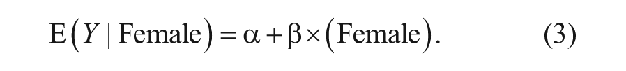
If we observe one boy with GPA of 2.0 and one girl with GPA of 4.0, an OLS model would estimate $\hat{α} = 3$ and $\hat{β} = 1$ , thereby fitting $E (Y | Female = 1) = 4.0$ and $E (Y | Female = - 1) = 2.0$ . This model would perfectly fit the training data. However, we might have a strong prior belief that boys and girls have similar GPAs. Thus, we might operationalize this principle by regularizing (shrinking) the estimates toward the sample mean. This approach would push $\hat{β}$ toward 0 unless the data strongly suggest otherwise. The benefit of regularization is that a few unexpected observations in the training sample (i.e., one boy with a 2.0 GPA) cannot greatly pull our predictions away from the general range where we expect them to fall (near the sample mean).

We could achieve regularization by adding a penalty term to the OLS loss function, using $\tilde{\vec{β}}$ to denote one candidate set of coefficients at which the loss function is evaluated:

L (\tilde{\vec{β}}, \vec{Y}) = \underset{Sum of squared error}{\underset{︸}{\sum_{i} {(Y_{i} - {\vec{X}}_{i}^{T} \tilde{\vec{β}})}^{2}}} + \underset{Penalty term}{\underset{︸}{λ \sum_{k} {\tilde{β}}_{k}^{2}}} .

(4)

The estimator $\hat{\vec{β}}$ would be the argument $\tilde{\vec{β}}$ that minimizes this loss function. In other words, instead of just minimizing the sum of the squared errors (first term), we would minimize the sum of the squared errors plus a penalty term that captures the complexity of the model (models with larger $\tilde{β}$ s are considered more complex). This model allows $\hat{\vec{β}}$ to move away from 0 only if doing so reduces the squared error term more than it increases the penalty term. This particular model (used by Roberts 2019) is called ridge regression and heavily penalizes coefficients that are very large. The penalty for moving $β_{1}$ from 0 to 1 is $λ$ , but the penalty for moving it from 1 to 2 is $(2^{2} - 1^{2}) λ = 3 λ$ . Ridge regression, therefore, regularizes away from very large parameter values. A similar approach—LASSO regression—uses a slightly different penalty term: the sum of the absolute values of the coefficients ( $λ \sum_{k} | β_{k} |$ ). For LASSO, the penalty for moving from 0 to 1 is the same as the penalty for moving from 1 to 2. The LASSO penalty can push some coefficients to exactly zero, thereby making it useful for variable selection. For instance, Stanescu et al. (2019) feed hundreds of variables to the LASSO algorithm and arrived at a prediction rule for material hardship that weighted only a handful of these variables, zeroing out those for which the contribution to prediction was insufficient to outweigh the addition to the penalty term. A third approach—elastic net regression—involves both a LASSO and a ridge penalty term and was used by many authors (e.g., Altscul 2019; Raes 2019; Rigobon et al. 2019; Roberts 2019).

By penalizing complex models (those with large $\hat{β}$ s), regularization reduces in-sample predictive performance but may improve out-of-sample predictive performance by preventing overfitting to the training data. A regularized approach, such as ridge regression, produces weights that are less likely to yield extreme predictions simply because of random variation in the training sample. Because it often helps improve out-of-sample predictive performance, regularization is widely used in applied machine learning and in this Special Collection.

In Equation 4, the parameter $λ$ controls the degree of regularization; $λ$ is often called a hyperparameter. Several authors in this Special Collection used models involving hyperparameters. Often, these authors learned the best hyperparameter by cross-validation (Table 7). They partitioned the data randomly into $k$ folds so that each observation was assigned to one fold. Then, they fit the model on all but one of these folds, assessed predictive performance on the remaining fold, and repeated with each fold left out in turn. By averaging across folds, this procedure yields an estimate of the out-of-sample predictive performance of the model with a given hyperparameter. This procedure makes it possible to learn a good hyperparameter value: the one that minimizes cross-validated MSE.

Tree-based methods

In addition to statistical learning approaches that used regularized regression, a second common family of approaches in the Special Collection was tree-based methods (Carnegie and Wu 2019; Compton 2019; McKay 2019; Raes 2019; Rigobon et al. 2019; Roberts 2019). Rather than assuming a particular function form for the relationship between predictors and outcomes, tree-based methods seek to learn the right functional form from the data. More concretely, tree-based methods place observations into groups and then produce the same prediction for everyone in the same group. The decision for how to split the observations into groups is data-driven and may use MSE as the loss function. While LASSO, ridge, and elastic net can only learn interactions and nonlinearities if the researcher explicitly includes them in the assumed function form, tree-based methods are able to discover nonlinearities and interactions from data without requiring the author to specify them in advance.

A hypothetical decision tree is shown in Figure 5. The first branch splits respondents into two groups: those whose mother completed college and those whose mother did not. Then, of those whose mother had completed college, the second branch separates respondents into two groups: whether the mother was younger than 23 or 23 and older when the child was born. This tree splits the population into three “leaves” and produces the same prediction for everyone in a given leaf, as depicted by the flat regions of the response surface plot.

Figure 5.

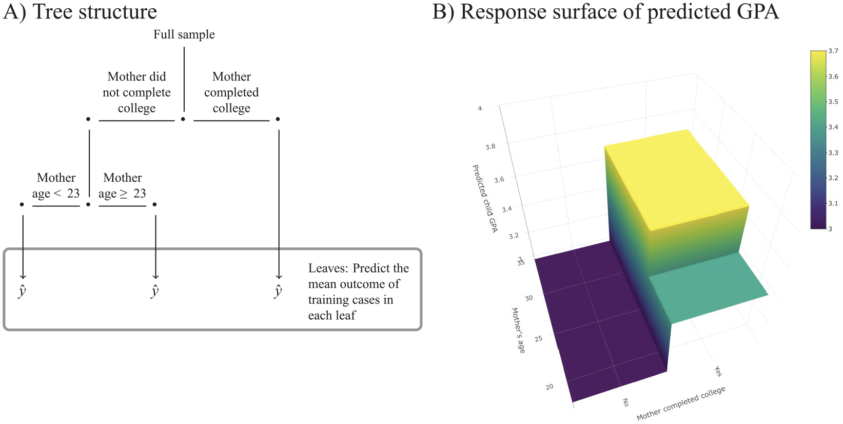
Example decision tree. Random forests, Bayesian additive regression trees, and gradient boosted trees are all extensions that combine many trees together.

Many algorithms have been proposed to create decision trees from data, and they generally involve efficient trial-and-error approaches for finding good splits for a given data set and outcome. Trees can capture complex interactions because the decisions along a branch may involve several different variables (e.g., mother’s education and mother’s age at birth). They can also flexibly approximate nonlinear associations; the ultimate response surface is locally flat with jumps where the covariates become part of a new leaf, like stair steps. For these reasons, trees are popular, flexible models. Raes (2019) and Roberts (2019) reported results from trees applied in this simplest form.

However, predictions that rely on a single tree can perform poorly because the tree learned can be very sensitive to the training sample (i.e., the tree would be very different if the training sample were slightly different). Three papers in this Special Collection used a generalization of trees called random forests to reduce this concern (Compton 2019; McKay 2019; Rigobon et al. 2019). By averaging over many trees, random forests produce an estimator with lower variance. To grow a tree, a random forest (1) samples rows of the data with replacement (also called a bootstrap sample) and (2) samples a subset of columns (variables) of the data without replacement. On this modified data set, the algorithm learns a decision tree. Then, it repeats the process hundreds or thousands of times, producing hundreds or thousands of decision trees. The sampling within each step ensures that the trees are all different from each other, thereby producing gains when these different trees are averaged together. For a new observation, each tree makes a prediction, and the forest averages all the predictions.

Raes (2019) and Rigobon et al. (2019) employed an approach adapted from random forests that often yields improved predictive performance: gradient boosted trees. Random forests train all trees in parallel: The decision rule learned by each tree is independent of all the other trees, given the data. Gradient boosted trees instead train each tree with the goal of correcting the prediction errors of prior trees. This procedure is often more computationally intensive but can yield improved predictive performance. In the context of the Challenge, Rigobon et al. (2019) achieved unusually strong predictive performance with gradient boosted trees.

Carnegie and Wu (2019) used a Bayesian adaptation of random forests: Bayesian additive regression trees (BART). The primary advantage of BART over other tree-based methods is that it enables Bayesian posterior inference (i.e., producing marginal effect point estimates and 95 percent credible intervals).

This section has introduced numerous approaches to statistical learning with a range of properties. Although distinct, all the approaches described previously follow the general framework of regression by accepting an input of predictors and returning a predicted value.

Model Interpretation

The fourth and final step in the four-step structure is model interpretation. For many papers in the Special Collection, understanding and describing the results of the statistical learning procedure is quite difficult. Researchers familiar with OLS may expect to fully describe a model by a small set of coefficients that capture how the predicted value of Y changes with a unit change in each given predictor, fixing all other predictors at constant values. When an OLS model includes squared terms or interactions, interpretation becomes more difficult because the conditional association between one variable and the outcome depends on either the initial value of that variable or the values of other variables. This is also true of generalized linear models, such as logistic regression, with or without interactions. This difficulty becomes more pronounced in statistical learning models that include many variables, complex nonlinearities, and high-level interactions. The number of parameters involved is often far too large to summarize the model parameters in a table.

Authors in this Special Collection were not required to interpret their models (see call for papers in the Supplemental Material), yet several offered interpretations. A few teams interpreted the model in terms of regression coefficients, thereby summarizing which variables had strong conditional associations with the outcome, given all the other variables in the model (Ahearn and Brand 2019; McKay 2019; Roberts 2019; Stanescu et al. 2019). Some teams also interpreted groups or clusters of variables, such as the contribution to predictive performance made by variables reported by the mother when the focal child was nine years old (Altschul 2019; Rigobon et al. 2019; Stanescu et al. 2019). Others interpreted how some hyperparameter (e.g., λ in Equation 4) played a central role in their prediction algorithm (Altschul 2019; Carnegie and Wu 2019).

Some manuscripts use algorithms that estimated variable importance (Altschul 2019; McKay 2019; Raes 2019; Rigobon et al. 2019; Roberts 2019). Although the definition of variable importance differed across algorithms, the general idea was to produce a single-number summary, analogous to a regression coefficient, to capture the contribution of a given predictor to the overall performance in a model in a way that might incorporate nonlinear and interactive relationships.

Benchmarks

Although the articles in the Special Collection used a variety of methods, they all shared the goal of predictive performance. Therefore, they frequently reported MSE or R² of their predictions. These predictions are assessed on one of four data sets: training, leaderboard with missing values imputed by random draws, leaderboard without missing values, and holdout. To contextualize the estimates reported in the Special Collection within the overall Challenge, Figure 6 shows the distribution of scores for each outcome for each data set.

Figure 6.

Empirical cumulative distribution function (CDF) of $R^{2}$ for all submissions with $R_{H o l d o u t}^{2} > 0$ . At each $R^{2}$ value (bottom axis), submissions with at most this $R^{2}$ value are represented as (left axis) a proportion and (right axis)a count. Top axis gives the corresponding mean squared error (MSE). To use this figure, find an $R^{2}$ or MSE value reported in a paper along the $x$ -axis. Move vertically to the intersection with the line on the $y$ -axis. Move left or right from this intersection to see the proportion or count of submissions with predictions worse than your reference point. The denominator of each $R^{2}$ calculation for a given evaluation set is the MSE of predicting the mean of training observations for all observations in that set. Empirical CDFs are truncated at $R^{2} = 0$ .

In addition to interpreting performance metrics in the context of the distribution observed in the Challenge, readers of this Special Collection should be aware of the important difference between training and holdout scores. During the Challenge, some submissions achieved $R_{Training}^{2}$ scores near 1, which suggests that these models made perfectly accurate predictions. However, when evaluated on the holdout set, the accuracy of these models typically dropped to close to 0 (Figure 7). Overall, the correlation between $R_{Training}^{2}$ and $R_{Holdout}^{2}$ was modest (ranging from .48 for material hardship to .05 for layoff), which emphasizes the importance of holdout data for fairly assessing model performance.

Figure 7.

Among submissions with $R_{H o l d o u t}^{2} > 0$ , training performance $R_{T r a i n}^{2}$ varied widely from 0 to 1 and was only modestly related to holdout performance. These results highlight the important distinction between predictive performance on data used to learn the model ( $R_{Train}^{2}$ ) and new data not used to learn the model ( $R_{Holdout}^{2}$ ). The denominator of each $R^{2}$ calculation for a given evaluation set is the mean squared error of predicting the mean of training observations for all observations in that set.

Conclusion

In addition to improving our understanding of the life course for children born in large U.S. cities, we hope that the Fragile Families Challenge and this Special Collection highlight the value of mass collaboration to advance social science research. In the natural sciences, large-scale collaborations already have led to important advances: Hundreds of biologists worked together to complete the first sequencing of the human genome (International Human Genome Sequencing Consortium 2001), and thousands of physicists worked together to find evidence of the Higgs boson (Aad et al. 2015). Although large-scale collaborations are becoming more common in psychology (Klein et al. 2018; Moshontz et al. 2018; Open Science Collaboration 2015), most research in the social sciences still happens individually or in small teams. There may, however, be some research problems in the social science where mass collaboration would create exciting, new possibilities.

Supplemental Material

Supplemental_Material – Supplemental material for Introduction to the Special Collection on the Fragile Families Challenge

Supplemental material, Supplemental_Material for Introduction to the Special Collection on the Fragile Families Challenge by Matthew J. Salganik, Ian Lundberg, Alexander T. Kindel and Sara McLanahan in Socius

Footnotes

Acknowledgements

We thank the Board of Advisors of the Fragile Families Challenge for guidance, and we thank Tom Hartshorne for research assistance.

Authors’ Note

The Fragile Families Challenge was approved by the Princeton University Institutional Review Board (No. 8061). The content of this paper is solely the responsibility of the authors and does not necessarily represent the views of anyone else.

Funding

The author(s) disclosed receipt of the following financial support for the research, authorship, and/or publication of this article: Research reported in this publication was supported by the Russell Sage Foundation, National Science Foundation (1760052), and the Eunice Kennedy Shriver National Institute of Child Health and Human Development of the National Institutes of Health under Award Nos. P2-CHD047879 and R24-HD047879. Funding for the Fragile Families and Child Wellbeing Study was provided by the Eunice Kennedy Shriver National Institute of Child Health and Human Development through Grants R01-HD36916, R01-HD39135, and R01-HD40421 and by a consortium of private foundations, including the Robert Wood Johnson Foundation. Alexander T. Kindel gratefully acknowledges funding support from a National Science Foundation Graduate Research Fellowship.

Supplemental Material

Supplemental material for this article is available with the manuscript on the Socius website.

1

2

Our submission platform was a modified version of CodaLab ().

3

For more on creating a reliable leaderboard score, see

4

When selecting the binary outcomes, we were guided by the advice of :356): “In research design, given the choice, one would prefer a single, abrupt, unexpected, short-lived treatment of dramatic proportions.”

5

If one of the papers reports an ${MSE}_{Holdout}$ and you would like to convert it into an $R_{Holdout}^{2}$ , here are the values that you can divide by: material hardship .025, GPA .425, grit .253, eviction .056, layoff .167, and job training .185.

Author Biographies

Matthew J. Salganik is a professor of sociology at Princeton University, and he is affiliated with several of Princeton’s interdisciplinary research centers: the Office for Population Research, the Center for Information Technology Policy, the Center for Health and Wellbeing, and the Center for Statistics and Machine Learning. His research interests include computational social science, social networks, and methodology. He is the author of Bit by Bit: Social Research in the Digital Age (Princeton University Press, 2018).

Ian Lundberg is a PhD candidate in sociology and social policy at Princeton University. His research focuses on the use of statistical and machine learning methods in the study of stratification and inequality. Beyond concerns about ethical data sharing, those seeking to apply new statistical developments face several hurdles: formalizing the estimand precisely in relation to a theoretical claim, stating and defending identification assumptions, and dealing with practical problems such as missing data. Lundberg’s research addresses these hurdles in substantive applications including the predictability of adolescent well-being, patterns of social mobility over multiple generations, the prevalence of housing eviction among U.S. children, and the effect of marriage on men’s wages. The common goal across these applications is to improve statistical practice in stratification and inequality research.

Alexander T. Kindel is a PhD student in sociology at Princeton University studying the organization, history, and practice of data analysis. His research interests include computational social science, historical sociology, and the sociology of knowledge.

Sara McLanahan is the William S. Tod Professor of Sociology and Public Affairs at Princeton University where she directs the Bendheim-Thoman Center for Research on Child Wellbeing. She is a principal investigator of the Fragile Families and Child Wellbeing Study and Editor-in-Chief of the Future of Children. Her research interests include family demography, intergenerational mobility, and inequality.

References

Aad

Georges

Abbott

Abdallah

Abdinov

Aben

Rosemarie

Abolins

Maris

AbouZeid

, et al. 2015. “Combined Measurement of the Higgs Boson Mass in pp Collisions at

\sqrt{s} = 7

and 8 TeV with the ATLAS and CMS Experiments.” Physical Review Letters 114(19):191803.

Ahearn

Caitlin E.

Brand

Jennie E

. 2019. “Predicting Layoff among Fragile Families.” Socius 5:1–8.

Altschul

Drew

. 2019. “Leveraging Multiple Machine Learning Techniques to Predict Major Life Outcomes from a Small Set of Psychological and Socioeconomic Variables: A Combined Bottom-Up/Top-Down Approach.” Socius 5:1–9.

Athey

Susan

. 2018. “The Impact of Machine Learning on Economics.” Pp. 115–46 in The Economics of Artificial Intelligence: An Agenda, edited by Agrawal

Gans

Goldfarb

. Chicago: University of Chicago Press.

Barocas

Solon

Selbst

Andrew D

. 2016. “Big Data’s Disparate Impact.” California Law Review 104:671.

Blau

Peter M.

Duncan

Otis Dudley

. 1967. The American Occupational Structure. Hoboken, NJ: John Wiley and Sons.

Blum

Avrim

Hardt

Mortiz

. 2015. “The Ladder: A Reliable Leaderboard for Machine Learning Competitions.” Pp. 1006 –1014 in Proceedings of the 32nd International Conference on Machine Learning, edited by Bach

Blei

. Lille, France: Microtome Publishing.

Breiman

2001. “Statistical Modeling: The Two Cultures.” Statistical Science 16(3):199–231.

Brier

Glenn W.

1950. “Verification of Forecasts Expressed in Terms of Probability.” Monthly Weather Review 78(1):1–3.

10.

Carnegie

Nicole B.

James

2019. “Variable Selection and Parameter Tuning for BART Modeling in the Fragile Families Challenge.” Socius 5:1–10.

11.

Chouldechova

Alexandra

Benavides-Prado

Diana

Fialko

Oleksandr

Vaithianathan

Rhema

. 2018. “A Case Study of Algorithm-Assisted Decision Making in Child Maltreatment Hotline Screening Decisions.” Pp. 134–48 in Proceedings of the 1st Conference on Fairness, Accountability and Transparency, edited by S. A. Friedler Wilson

. New York, NY: ACM.

12.

Compton

Ryan

. 2019. “A Data-Driven Approach to the Fragile Families Challenge: Prediction through Principal Components Analysis and Random Forests.” Socius 5:1–7.

13.

Courtland

Rachel

. 2018. “Bias Detectives: The Researchers Striving to Make Algorithms Fair.” Nature 558(7710):357.

14.

Davidson

Thomas R.

2019. “Black-Box Models and Sociological Explanations: Predicting High School GPA Using Neural Networks.” Socius 5:1–11.

15.

Desmond

Matthew

Gromis

Ashley

Edmonds

Lavar

Hendrickson

James

Krywokulski

Katie

Leung

Lillian

Porton

Adam

. 2018. Eviction Lab National Database: Version 1.0. Princeton, NJ: Princeton University. www.evictionlab.org.

16.

Desmond

Matthew

Kimbro

Rachel Tolbert

. 2015. “Eviction’s Fallout: Housing, Hardship, and Health.” Social Forces 94(1):295–324.

17.

Donoho

David

. 2017. “50 Years of Data Science.” Journal of Computational and Graphical Statistics 26:745–66.

18.

Duckworth

Angela L.

Peterson

Christopher

Matthews

Michael D.

Kelly

Dennis R

. 2007. “Grit: Perseverance and Passion for Long-Term Goals.” Journal of Personality and Social Psychology 92(6):1087.

19.

Dunn

Lloyd M.

Dunn

Douglas M

. 2007. PPVT-4: Peabody Picture Vocabulary Test. Bloomington, MN: Pearson Assessments.

20.

Efron

Bradley

Hastie

Trevor

. 2016. Computer Age Statistical Inference: Algorithms, Evidence, and Data Science. Cambridge, UK: Cambridge University Press.

21.

Eubanks

Virginia

. 2018. Automating Inequality: How High-Tech Tools Profile, Police, and Punish the Poor. New York: St. Martin’s Press.

22.

Filippova

Anna

Gilroy

Connor

Kashyap

Ridhi

Kirchner

Antje

Morgan

Allison C.

Polimis

Kivan

Usmani

Adaner

Wang

Tong

. 2019. “Humans in the Loop: Incorporating Expert and Crowdsourced Knowledge for Predictions Using Social Survey Data.” Socius 5:1–15.

23.

Friedman

Jerome

Hastie

Trevor

Tibshirani

Robert

. 2001. The Elements of Statistical Learning. New York: Springer.

24.

Goode

Brian J.

Datta

Debanjan

Ramakrishnan

Naren

. 2019. “Imputing Data for the Fragile Families Challenge: Identifying Similar Survey Questions with Semi-automated Methods.” Socius 5:1–6.

25.

Hofman

Jake M.

Sharma

Amit

Watts

Duncan J

. 2017. “Prediction and Explanation in Social Systems.” Science 355(6324):486–88.

26.

International Human Genome Sequencing Consortium. 2001. “Initial Sequencing and Analysis of the Human Genome.” Nature 409(6822):860.

27.

Kindel

Alexander

Bansal

Vineet

Catena

Kristin

Hartshorne

Thomas

Jaeger

Kate

Koffman

Dawn

McLanahan

Sara

Phillips

Maya

Rouhani

Shiva

Vinh

Ryan

Salganik

Matthew J

. 2019. “Improving Metadata Infrastructure for Complex Surveys: Insights from the Fragile Families Challenge.” Socius 5:1–24.

28.

Klein

Richard A.

Vianello

Michelangelo

Hasselman

Fred

Adams

Byron G.

Adams

Reginald B.

Jr. Alper

Sinan

Aveyard

Mark

, et al. 2018. “Many Labs 2: Investigating Variation in Replicability across Samples and Settings.” Advances in Methods and Practices in Psychological Science 1(4):443–90.

29.

Kleinberg

Jon

Ludwig

Jens

Mullainathan

Sendhil

Obermeyer

Ziad

. 2015. “Prediction Policy Problems.” American Economic Review 105(5):491–95.

30.

Lakkaraju

Himabindu

Kleinberg

Jon

Leskovec

Jure

Ludwig

Jens

Mullainathan

Sendhil

. 2017. “The Selective Labels Problem: Evaluating Algorithmic Predictions in the Presence of Unobservables.” Pp. 275–84 in Proceedings of the 23rd ACM SIGKDD International Conference on Knowledge Discovery and Data Mining. New York: ACM.

31.

Lundberg

Ian

Donnelly

Louis

. 2019. “A Research Note on the Prevalence of Housing Eviction among Children Born in US Cities.” Demography 56(1):391–404.

32.

Lundberg

Ian

Narayanan

Arvind

Levy

Karen

Salganik

Matthew J

. 2019. “Privacy, Ethics, and Data Access: A Case Study of the Fragile Families Challenge.” Socius 5:1–25.

33.

McKay

Stephen

. 2019. “When 4 ≈ 10,000: The Power of Social Science Knowledge in Predictive Performance.” Socius 5:1–7.

34.

Molina

Mario

Garip

Filiz

. 2019. “Machine Learning for Sociology.” Annual Review of Sociology 45:27–45.

35.

Moshontz

Hannah

Campbell

Lorne

Ebersole

Charles R.

IJzerman

Hans

Urry

Heather L.

Forscher

Patrick S.

Grahe

Jon E.

, et al. 2018. “The Psychological Science Accelerator: Advancing Psychology through a Distributed Collaborative Network.” Advances in Methods and Practices in Psychological Science 1(4):501–15.

36.

Mullainathan

Sendhil

Spiess

Jann

. 2017. “Machine Learning: An Applied Econometric Approach.” Journal of Economic Perspectives 31(2):87–106.

37.

Open Science Collaboration. 2015. “Estimating the Reproducibility of Psychological Science.” Science 349(6251):aac4716.

38.

Raes

Louis

. 2019. “Predicting GPA at Age 15 in the Fragile Families and Child Wellbeing Study.” Socius 5:1–8.

39.

Reichman

Nancy E.

Teitler

Julien O.

Garfinkel

Irwin

McLanahan

Sara S

. 2001. “Fragile Families: Sample and Design.” Children and Youth Services Review 23(4–5):303–26.

40.

Rigobon

Daniel

Jahani

Eaman

Suhara

Yoshihiko

Al-Ghoneim

Khaled

Alghunaim

Abdulaziz

Pentland

Alex

Almaatouq

Abdullah

. 2019. “Winning Models for GPA, Grit, and Layoff in the Fragile Families Challenge.” Socius 5:1–10.

41.

Roberts

Claudia V.

2019. “Friend Request Pending: A Comparative Assessment of Engineering and Social Science Inspired Approaches to Analyzing Complex Birth Cohort Survey Data.” Socius 5:1–8.

42.

Rosenbaum

Paul R

. 2002. Observational Studies. 2nd edition. New York: Springer.

43.

Salganik

Matthew J.

Lundberg

Ian

Kindel

Alexander T.

Ahearn

Caitlin E.

Al-Ghoneim

Khaled

Almaatouq

Abdullah

Altschul

Drew M.

et al. 2020. “Measuring the Predictability of Life Outcomes with a Scientific Mass Collaboration.” Proceedings of the National Academies of Sciences. https://doi.org/10.1073/pnas.1915006117.

44.

Särndal

Carl-Erik

Swensson

Bengt

Wretman

Jan

. 2003. Model Assisted Survey Sampling. New York: Springer Science & Business Media.

45.

Shmueli

Galit

. 2010. “To Explain or to Predict?” Statistical Science 25(3):289–310.

46.

Stanescu

Diana

Wang

Erik

Yamauchi

Soichiro

. 2019. “Using LASSO to Assist Imputation and Predict Child Wellbeing.” Socius 5:1–21.

47.

Torche

Florencia

. 2015. “Analyses of Intergenerational Mobility: An Interdisciplinary Review.” The Annals of the American Academy of Political and Social Science 657(1):37–62.

48.

Yarkoni

Tal

Westfall

Jacob

. 2017. “Choosing Prediction over Explanation in Psychology: Lessons from Machine Learning.” Perspectives on Psychological Science 12(6):1100–22.

Supplementary Material

Please find the following supplemental material available below.

For Open Access articles published under a Creative Commons License, all supplemental material carries the same license as the article it is associated with.

For non-Open Access articles published, all supplemental material carries a non-exclusive license, and permission requests for re-use of supplemental material or any part of supplemental material shall be sent directly to the copyright owner as specified in the copyright notice associated with the article.

0.00 MB

0.07 MB