
Abstract
We propose a measure of discursive holes well suited for the unique properties of text networks built from document similarity matrices considered as dense weighted graphs. In this measure, which we call textual spanning, documents similar to documents dissimilar from one another receive a high score, and documents similar to documents similar to one another receive a low score. After offering a simulation-based validation, we test the measure on an empirical document similarity matrix based on a preestimated topic-model probability distribution. The results demonstrate that our proposed textual spanning measure captures different structural features of discursive fields than alternative measures.
Introduction
Building on Breiger’s (1974) formalization of Simmel’s (1955) idea of the duality of persons and groups, relational approaches have proliferated in cultural sociology (Mohr 1998; Mohr and Duquenne 1997; Mützel 2009), economic sociology (Bandelj 2015; Fourcade 2007; Stoltz 2018), political sociology (Mische 2000; Tilly 2001), and other fields (Emirbayer 1997; Mische 2011; Smith-Lovin 1999). Surveying this work, one finds the “relations” involved are highly diverse. Indeed, one of the strengths of the relational approach is that analysts can be agnostic as to what constitutes a relation, allowing more specific theoretical and empirical criteria to drive selection. Analysts can then treat these networks as a social field (or ecology), projecting the result into more interpretable low-dimensional spaces. This brings together field-theoretic and ecological approaches, sharing a common spatial metaphor (Liu and Emirbayer 2016), with network methods originally designed to measure the structure of social relations between individuals.
In this vein, a “discursive field” may be an autonomous field (e.g., a literary genre) or a particular dimension of a social field (e.g., a medium through which corporations communicate) and conceptualized as a multidimensional space of positions defined by similarities and dissimilarities among texts or text producers (Bail 2016). Advancing such a relational approach for the study of discourse, we propose a simple and intuitive technique for measuring the “holes” in discursive fields (Pachucki and Breiger 2010; Vilhena et al. 2014) by identifying texts (or text producers) that span more or less “textual distance.” We remain agnostic about the substantive uses of the patterns emerging from our proposed technique, but we outline its broader utility in the conclusion.
In our proposed measure, documents closely related to documents that are not also closely related to each other receive a high score, whereas documents related to other “redundant” documents with strong mutual similarities receive a low score. After offering a simulation-based validation of our measure, we test it using a document similarity matrix based on a previously published (and openly available) preestimated topic-model probability distribution using the CMU 2008 Political Blog Corpus (Eisenstein and Xing 2010; Roberts, Stewart, and Tingley 2015). It is important to note that how one constructs his or her text network—whether constructing it from a topic-model solution, raw counts, term frequency–inverse document frequency (TF-IDF) scores, and so on—is of crucial importance when interpreting what our proposed measure means in any given substantive context. We use topic modeling to construct our network simply given its current popularity in sociology, the ease with which general interpretations can be derived from them, and because the CMU 2008 Political Blog Corpus offers a preestimated topic-model solution.
Finding Documents Spanning Discursive Holes
One way of thinking about whether a document spans a greater or lesser distance in a discursive field is to simply take the row sum of a document-by-document similarity matrix as the cumulative distance for each document: the greater the sum, the greater the distance. Following Freeman’s (1978) original formulation, this would be a document’s degree centrality, or more accurately for weighted networks, a document’s vertex strength (Barrat et al. 2004). One drawback of this approach is that it presumes only direct ties between the focal and other documents matter while ignoring the relations between these other documents. Another intuitively appealing strategy would be to compute the document betweenness centrality in the similarity network. This metric would assess the extent to which a document lies on the largest number of shortest paths between any other pair of documents. A noted problem with shortest paths–based measures, however, is that they lead to a high number of zero counts, especially in dense or fully connected similarity networks such as the ones under consideration here (Opsahl, Agneessens, and Skvoretz 2010). This renders them of limited use for identifying gradations in textual spanning.
Combining some of the underlying intuitions of these approaches, we propose that an ideal textual spanning measure should take into account similarities between the focal document and other documents in the network such that a document that is similar to other documents not similar to one another spans a greater distance. The same measure should be at a minimum when a focal document is very similar to other documents that are also very similar to one another.
Such a measure is informed by Granovetter’s (1973) strength of weak ties argument, itself building on Rapaport and Horvath’s (1961:290) claim that “one would expect the friendship relations, and therefore the overlap bias of the acquaintance circles, to become less tight with increasing numerical rank-order.” The main idea here is that closer contacts, for example, friends, are more likely to know each other than more distant contacts, for example, co-workers and acquaintances. Therefore, if one wants novel information, one is better off connecting to these more distant contacts. Burt (1992) later isolated the key mechanism, noting valuable information is more likely to be obtained from weak ties precisely because weak ties are more likely to span “structural holes.” As not all weak ties span structural holes, however, one should focus on the latter. Burt formalized this insight by proposing a measure of the redundancy of one’s contacts, or the extent one’s contacts know each other and therefore are likely to provide access to similar information and resources.
Following Lizardo’s (2014) generalization of Burt’s measure of network efficiency to measure cultural omnivorousness, we apply a modified version of Burt’s constraint scores to measure textual spanning in document similarity networks. There are two primary differences between our measure of textual spanning and constraint: (1) We incorporate recent advances in weighted network metrics to calculate each individual node’s similarity to its local neighborhood, and (2) each node’s similarity to its neighborhood is inversely related to the similarity of its neighbors’ neighborhood.
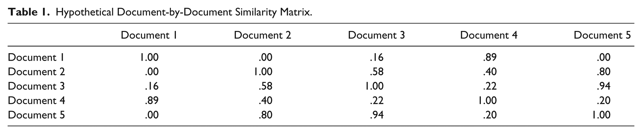
As a brief illustration, consider the hypothetical document-by-document similarity matrix in Table 1 and rendered as a network graph in Figure 1. In this text network, Document 4 is the biggest textual spanner. Specifically, it has similarities to both Document 2 and Document 1, which in this example have no similarities to each other.
Hypothetical Document-by-Document Similarity Matrix.

Text network based on Table 1.
A document-by-document similarity matrix (like Table 1) can be thought of as a weighted adjacency matrix. Again, how similarities between documents is measured is an important theoretical consideration. Therefore, in the hypothetical example, these similarities could be thought of as, for instance, total proportion of shared words between documents. This matrix in turn can be represented as a graph (like Figure 1) with the individual documents as nodes and the similarities represented as weighted connections.
Textual Spanning: Identifying Documents Bridging Discursive Holes
With the aforementioned theoretical and formal motivation in mind, we define a document’s cumulative textual spanning
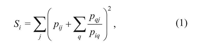
where

The second term in Equation 1,
Finally, to make the measure more interpretable, we standardize the output by taking the z score of each
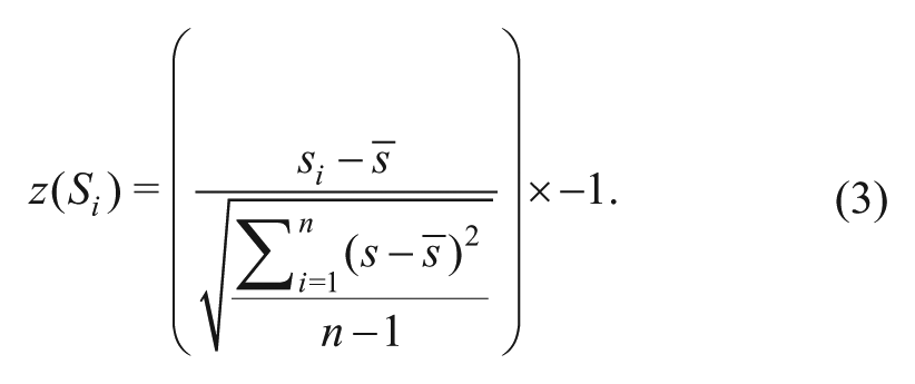
It is important to emphasize that standardization does not permit cross-network comparisons unless the network-specific spanning score variances,
We used the R statistical computing environment (Core R Team 2013) to perform the analyses (the function implementing the aforementioned measure of textual spanning is written in Base R and provided in the Appendix).
Simulated Examples
Most text networks will be fully connected weighted graphs and therefore dense, rather than sparse, matrices. Each text (of the same language at least) would have a minimal similarity to another text. However, the method used to preprocess and compare texts may allow for the possibility of no similarity—for example, by binning very low similarities or engaging in liberal removal of very common words. However, the textual spanning measure is not as effective on disconnected graphs, as demonstrated by two simulated eight-node networks (see Figure 2). One has tie strengths set at various levels from .95 to .05 but is fully connected. The other reduces all tie strengths of the first by .05, producing a few zero edges. Importantly, one node has a higher degree than the rest. The final graphs are small-world networks based on a rewiring algorithm (Watts and Strogatz 1998). As the methods used to measure similarities between documents vary, the tie strengths in these simulated networks can be interpreted as, for example, overall proportion of shared words or thematic similarities derived from topic modeling.

Textual spanning and degree for fully connected and disconnected graphs.
In the top row, the two nodes rendered in vibrant blue are high-spanning documents as they connect the bulk of the network (the less blue, more gray nodes) to otherwise weakly connected documents (yellow nodes). The gray nodes, while well connected to each other and therefore fairly similar to the corpus overall, offer little in terms of spanning dissimilar documents. Importantly, the node with the highest degree (the top center node) and the lowest degree (bottom right node and center right node) are not the highest spanners for the connected graph. However, in the disconnected graph, the lowest degree nodes become the highest spanners—indicating there may be a weak correlation between degree and spanning on disconnected graphs.
Next, we consider a discursive field with two densely connected cliques. This could, for example, represent political polarization or distinct fictional genres, where texts are quite similar within each clique but not very similar between each clique. In such a network, some documents may attempt to span across each clique (the blue node in Figure 3) by, for instance, blending or comparing texts and provide the clearest examples of spanning a hole in a discursive field.
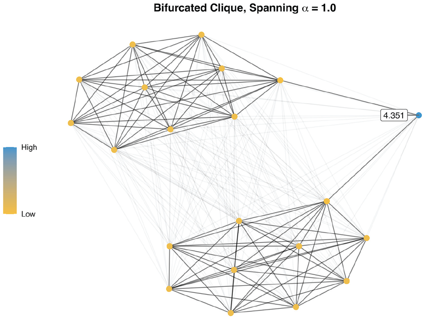
Textual spanning on simulated network data with two dense components.
Finally, consider a simulated core-periphery text network (Figure 4). In this case there is a closely linked group of producers which are similar to each other (the yellow nodes) and somewhat disconnected producers which are only weakly similar to each other. Although some of the core producers are “bridging,” only the peripheral producers are the highest spanners. This suggests that the measure is affected by certain network topologies.

Textual spanning on simulated network data with core-periphery structure.
Empirical Example
As an empirical illustration, we use a preestimated topic-model solution of the CMU 2008 Political Blog Corpus (Eisenstein and Xing 2010; Roberts et al. 2015). Topic modeling is an approach that is gaining considerable popularity in sociology (Mohr and Bogdanov 2013). We motivate this section via a simple proposition: A topic-model solution, as a probability distribution of documents over a discrete latent topic structure, can be conceptualized as a document-topic affiliation network (see also Gerlach, Peixoto, and Altmann 2018). By treating these document-topic distributions as two-mode relational data, network metrics can be used to identify discursive holes and the vertices occupying them.
Topic Modeling and the Document-Topic Probability Distribution
Conceptually speaking, a topic model can be understood as a type of multilevel factor analysis for uncovering the thematic structure of a finite set of unstructured (i.e., nonnumeric) discrete data, such as text. “The basic idea is that documents are represented as random mixtures over latent topics,” Blei, Ng, and Jordan (2003:996) write, “where each topic is characterized by a distribution over words.”
The raw output of a topic model of a text corpus is “a generative probabilistic model of [the] corpus” (Blei et al. 2003:996), comprising two probability distributions: a probability distribution of topics over weighted words and a probability distribution of documents over weighted topics. Documents are therefore understood as “bags of words,” where a document’s allocation to a particular topic within the larger latent topic structure (i.e., the probability distribution of documents over topics) can be interpreted as the percentage chance that a word drawn at random from that bag of words (the document) will belong to that topic given that term’s weight in the topic-word probability distribution. Given the interest here in documents as the unit of analysis, the remainder of this paper focuses on the document-topic probability distribution rather than the topic-word probability distribution. (For a detailed mathematical account of latent Dirichlet allocation, see Blei et al. 2003:996–99.)
Topic-model analyses typically begin with a description of the latent topic structure found in the corpus. Consider, for example, Figure 5, the results of a structural topic-model analysis on a corpus of over 13,000 political blogs from 2008 (Roberts et al. 2015)—a collection of documents we discuss in a bit more detail later. The topics, of which there are 20, are arrayed in descending order of prevalence across the corpus and show the marginal expected topic proportions.

Typical presentation of topic model results.
The three terms associated with each topic are the three terms with the highest probability of being associated with that topic. 3 As an interpretation example, consider Topic 3. The top three words associated with the topic are obama, barack, and campaign, suggesting this is a “2008 Obama Campaign” topic. It is the third largest topic, with a little over 5 percent chance that a random word selected from a random blog post in the corpus will be associated with talk of Obama’s 2008 presidential campaign.
We can examine the document-topic probability distribution by itself to look at topics at the document level. Table 2 provides the probability distribution of the first five documents from the corpus over the latent topic structure from Figure 5.
Sample Distribution from STM Solution with CMU 2008 Political Blog Data.

Note: This is a sample of the first five blogs in the corpus. Total NDocuments = 13,246. Probabilities from Roberts, Stewart, and Tingley (2015) topic-model analysis.
Following the assumptions of a Bayesian Dirichlet-multinomial distribution, each document (

The interpretation of Table 2 is straightforward. For instance, about 48 percent of Document 2 terms are accounted for by Topic 1—meaning almost half of the total words in Document 2 are allocated to talk of presidential polling analysis.
The core takeaways of this brief conceptual topic-model primer are as follows. First, topic modeling provides insight into the latent topic structure of the document corpus. Second, documents are modeled as probabilities across this latent topic structure, where each document must sum to 1 across the topics. It is this document-topic probability distribution that we argue can be treated as two-mode relational data from which we can build a document-by-document weighted adjacency matrix.
Now that we have a document-by-topic probability matrix, with each document represented as a row vector of probabilities over topics, we can compare any two documents in the corpus by how similar their respective vectors are. In text analysis more broadly, this is most commonly accomplished by taking the cosine of the two vectors and is also popular for assessing document similarities in topic-model contexts (for a few examples, see Liu, Niculescu-Mizil, and Gryc 2009; Tian, Revelle, and Poshyvanyk 2009; Wu 2013). 4 This is defined as the dot product of the two vectors divided by the product of the lengths of both vectors.
If we take the cosine of the document-by-topic matrix, we would get a topic-by-topic matrix with similarities between each topic domain. As we want a document-by-document similarity matrix, we take the cosine of the transpose of the matrix and arrive at matrix of similarities between documents based on their topic vector distributions. We can now easily think of this as a weighted adjacency matrix and apply network thinking.
Measuring Document Position in a Discursive Field
In Figure 6, for ease of computation and representation, we plot a random sample of 100 blog posts from the preestimated topic models of the CMU 2008 Political Blog Corpus (Eisenstein and Xing 2010; Roberts et al. 2015). We scale each vertex by the length of the post in terms of word counts (post text preprocessing; see Note 2). We also label vertices with their respective spanning scores for those that are greater than or equal to the 95th percentile and those less than or equal to the 1st percentile. In the visualization, we remove edges that are below .6 to aid interpretation, but recall this is actually a fully connected graph.

Identifying discursive holes in the CMU 2008 Political Blog Corpus.
As to be expected, this yields a much more complicated network structure than in the simulated data. There are both clique and core-periphery elements of the network where some spanners are reaching out from the core of cliques while others are bridging across components. We compare our textual spanning measure to other measures of centrality in weighted networks as defined by Opsahl et al. (2010): weighted degree, weighted betweenness, and weighted closeness. We calculated these measures using the tnet R package (Opsahl 2007).
Because the relative length of a document logically increases the chances it will span greater discursive distance, we also compare our measure to length by summing the total word count for each blog post. The results are presented in Figure 7, and the bivariate Pearson correlation coefficients and bivariate scatterplots are shown in Figure 8.

Comparing document position metrics.
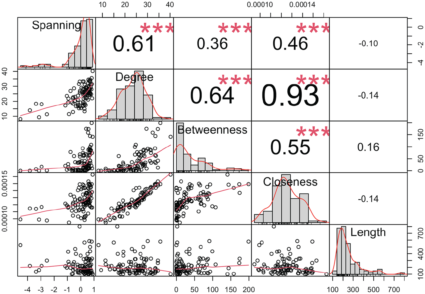
Bivariate pearson correlations and scatterplots.
The results of the comparison demonstrate that textual spanning is identifying structural features of the discursive field that standard centrality measures miss. The strongest correlation is that between spanning and weighted degree, which is reasonable considering that documents that have more similarities to a corpus overall would be more likely to span greater distances (however, this relationship can be weakened by decreasing the tuning parameter to below 1; see Note 1).
The two shortest path measures, betweenness and closeness, are only weakly correlated with the spanning measure, and specifically for betweenness, there are a high number of vertices with a score of zero. While all measures are very weakly correlated with document length, this is partially the result of basing the document-by-document similarity matrix on the topic-model probability solution. Alternative measures of document similarity, such as those based on term frequency or even word embeddings, would likely yield somewhat stronger correlations.
But of what substantive significance is the fact that this textual spanning measure appears to be picking up on structural features missed by the other centrality measures? To answer this question, we isolated the five blog posts with the highest spanning scores and compared those scores to their respective weighted degree, weighted betweenness, and weighted closeness centralities. Figure 9 displays the standardized distribution of each centrality measure, with black triangles indicating the five blog posts with the highest textual spanning scores and where they fall across the metrics. The top five posts are, of course, at the very top of the spanning distribution; importantly though, these five posts are not as readily identified as central documents across the other measures, with each of the other three measures placing at least one of the posts below their respective medians.

Comparing where top five spanning posts fall across centrality measures.
Consider, for example, a post with a high textual spanning score (in the top quartile) but relatively low scores across the other centrality measures: post No. 12,698, a post from the liberal Talking Points Memo blog, published October 2, 2008. The post was the 24th largest spanning document (
Unsurprisingly, the post loaded highest on topic Nos. 18 (about John McCain’s presidential campaign) and 14 (about American work, jobs, and labor). In the case of topic-model similarity networks, our textual spanning measure should be used to identify posts bridging two or more posts that do not engage in the same topics with same levels of emphasis: For example, post No. 12,698 might be a high spanner because it is connecting these two topics, “McCain presidential campaign” and “American work, jobs, and labor,” which are otherwise not frequently co-discussed across other posts in the corpus. Figure 10 displays a weighted correlation network between the 20 topics in the sample, with only positive correlations at or above 0.1 shown. An edge suggests the two linked topics are frequently co-discussed. As the figure shows, the McCain campaign topic (topic No. 18, yellow) and American work topic (topic No. 14, yellow) are in fact not frequently discussed together in the same posts. Therefore, post No. 12,698 appears to be a high spanner in part because it engages both of these topics, thereby bridging posts that tend to engage in one but not the other. This spanning dynamic is not captured by the weighted centrality measures precisely because these topics are rarely talked about together in other posts—that is, this combination makes this post dissimilar to others and thus penalizes its edge strength with other posts.
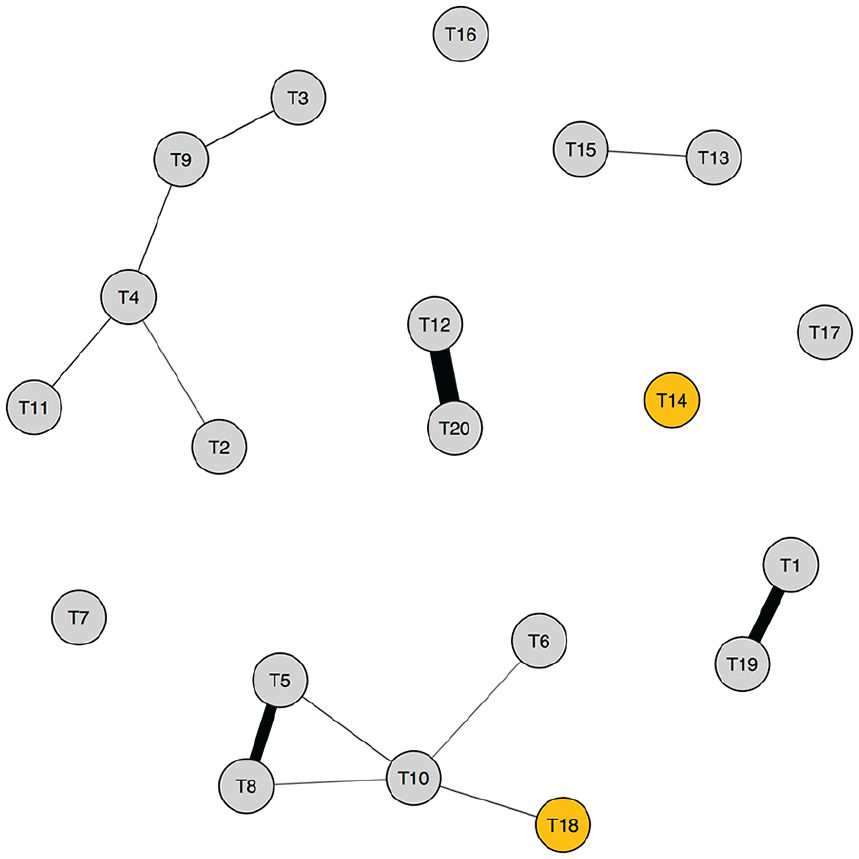
Topic correlation network.
Conclusion
We proposed a measure of textual spanning that increases when a document is closely related to documents that are not also closely related to each other (and vice versa). This measure is particularly well suited for the unique properties of text networks built from document similarity measures, which tend to be dense weighted graphs. Furthermore, this measure is useful regardless of the length of documents in a corpus (e.g., social media posts or articles). The only requirement to apply our measure of textual spanning is a document-by-document (or text producer–by–text producer) similarity matrix.
The analyst can begin with any vectorizing technique, such as a basic document-by-term frequency matrix or TF-IDF weighted matrices (Salton and Buckley 1988; Salton, Wong, and Yang 1975; Wu and Salton 1981). Our measure can even be applied to more advanced word-embeddings techniques (Kozlowski, Taddy, and Evans 2018; Mikolov, Yih, and Zweig 2013), specifically using Word Mover’s Distance (Kusner et al. 2015) to generate a document-by-document similarity matrix. It is important to emphasize that how one defines the boundaries of the corpus and builds the text network is a crucial step in interpreting the meaning of textual spanners. For example, topic models identify generic thematic categories, whereas word embeddings are better suited for more fine-grained lexical patterns. Which approach is used, however, should be a theoretically driven decision.
If the data allow us to assume author independence between documents in the corpus, or documents can be aggregated by producer, this can create a producer-by-producer similarity matrix (Bail 2016; Godart 2018). Therefore, our measure may also be used to identify collective actors, such as social movement organizations, corporations, or news organizations, as spanners of more or less distances in a discursive field. For example, textual spanning may be used to locate what Bail (2016) refers to as “cultural bridges” built by advocacy organizations. Similarly, an analyst may take the text about cultural objects, such as reviews of music and movies, to infer the extent to which cultural objects span greater discursive distances.
There are many reasons an analyst might wish to identify these distance-spanning documents, cultural objects, or producers in discursive fields. Researchers may derive information about, for example, cultural fit, creativity, innovation, ideational diversity, classification ambiguity, ideological polarization, or unique coalitions between individuals and organizations. Therefore, we believe textual spanning is broadly useful across various subfields in the social sciences.
Footnotes
Appendix
Acknowledgements
We would like to thank the editors and anonymous reviewers at Socius for their helpful feedback. We would also like to extend gratitude to Omar Lizardo, Terry McDonnell, Erin McDonnell, Michael Lee Wood, and all the members of the Notre Dame Culture Workshop for their comments on earlier drafts of this paper. Code for reproducing the analyses and figures in this paper are publicly available at the following GitHub repository: ![]() .
.
1
Increasing
2
This is a key difference between textual spanning and Burt’s constraint as the latter is multiplicative: ![]() :321) words, constraint “varies from 0 to 1 with the extent to which
:321) words, constraint “varies from 0 to 1 with the extent to which
3
As the terms show, the corpus has also been “preprocessed.” For the Roberts, Stewart, and Tingley (2015) analysis, punctuation, capitalization, stop words (e.g., conjunctions and prepositions), numbers, words less than three characters long, words that appear in only one document, and excess white space were removed, and words were stemmed (see ![]() ).
).
4
The reason cosine similarity is the preferred measure is because the raw dot product is higher if a vector is longer. Dividing by the vectors’ lengths normalizes the measure, resulting in a larger number if the documents are more similar, and vice versa, regardless of the lengths of the vectors. This is much more important for analyses based on document-term matrices and less so for our approach here using document-topic probability matrices since the length of the vector is set to the number of topics where each document-topic cell entry is nonzero.