Sage Journals: Discover world-class research

Abstract

The Fragile Families Challenge provided an opportunity to empirically assess the applicability of black-box machine learning models to sociological questions and the extent to which interpretable explanations can be extracted from these models. In this article the author uses neural network models to predict high school grade point average and examines how variations of basic network parameters affect predictive performance. Using a recently proposed technique, the author identifies the most important predictive variables used by the best performing model, finding that they relate to parenting and the child’s cognitive and behavioral development, consistent with prior work. The author concludes by discussing the implications of these findings for the relationship between prediction and explanation in sociological analyses.

Keywords

prediction grade point average neural networks machine learning cross-validation

The Fragile Families Challenge (FFC) was a competition held in 2017 to bring together social scientists and data scientists in a mass collaboration to predict six outcome variables in the Fragile Families and Child Wellbeing Survey (Reichman et al. 2001). Participants were able to use data from waves 1 through 5 of the survey, which cover the period from each child’s birth until age 9, to predict outcomes at age 15. The aim of the FFC was to assess how well these outcomes could be predicted and to help uncover new determinants of these outcomes for further assessment using in-depth interviews (Salganik et al. 2019). As part of the FFC, I evaluated the performance of neural network models for predicting self-reported high school grade point averages (GPAs). In this article I detail the process of constructing, testing, and evaluating these models. I also build upon recent calls to reconcile predictions and explanations (Hofman, Sharma, and Watts 2017) by applying a recently proposed method to help explain the predictions of these black-box models (Ribeiro, Singh, and Guestrin 2016). Consistent with prior work, variables related to parenting, cognitive, and behavioral development, as well as the school, the family, and the community, appear to be important predictors of educational success.

In the “Background” section, I begin by discussing prediction, machine learning, and their implications for the explanatory mode of analysis favored by sociologists. I then give a general introduction to neural network models. This is followed by a short review of the literature on the determinants of educational performance and prior work predicting high school GPA. In the “Methods” section, I describe the process of cleaning and transforming the FFC data, then training and evaluating the neural network models. The “Results” section consists of two parts. In the first I evaluate the predictive performance of the different models tested; in the second I introduce and apply a method to interpret the predictions made by the neural network and assess how the results relate to prior work. I conclude the article by reflecting on the results and the remaining obstacles that must be addressed if we are to reconcile predictive modeling with sociological explanations.

Background

Prediction and Sociological Explanations

Watts (2014) argued that common-sense thinking is pervasive in sociological reasoning, resulting in a bias toward parsimonious accounts of social life that are commensurable with our everyday experiences but that may not be scientifically valid. To help ensure the validity of our explanations, Watts advocated a shift away from evaluating them on the basis of their understandability and toward their capacity to predict, which can be assessed using out-of-sample testing. Although the focus of Watts’s article is on using prediction as a way to evaluate our explanations, prediction can also be valuable as an end in itself. The machine-learning models and techniques used by computer scientists and other practitioners are well suited to this task because they provide efficient ways to make data-driven predictions and to reliably assess their accuracy and validity.¹

A limitation of these models is that they are often considered “black boxes,” meaning that we do not directly observe how they work (cf. Hedström and Swedberg 1998), making them incompatible with the types of explanations preferred by many sociologists (e.g., Turco and Zuckerman 2017). However, the increasing ubiquity of machine-learning models and their use in consequential decisions in domains including health care and criminal justice (Athey 2017) is leading many researchers to develop techniques to help us better understand them. Although most machine learning models are not transparent, in the sense that their inner workings are clear to observers, this does not imply that they are not interpretable (Lipton 2016). For example, methods have recently been proposed to allow us to obtain post hoc interpretations for any class of model (Lundberg and Lee 2017; Ribeiro et al. 2016). Reflecting upon these trends, Hofman et al. (2017) concluded their recent Science article by stressing that “the trade-off between predictive accuracy and interpretability may be less severe than once thought” (p. 488).

However, there is reason to be skeptical that models optimized for prediction can also provide us with valid explanations. The dominant framework in supervised machine learning is to start with a large data set and feed it into a model that finds a functional form to optimize for predictive accuracy. Mullainathan and Spiess (2017) contended that because these models are optimized to estimate $\hat{y}$ values with high accuracy, rather than consistently estimate a set of $\hat{β}$ values, we cannot reliably use them to interpret the latter as is the norm in the explanatory models used by social scientists. When a predictive model uses a large number of variables, often greater than the number of observations, they argue that the most important variables identified are typically a subset of a larger set of variables that are associated with the outcome. “The very appeal of these algorithms is that they can fit many different functions. But this creates an Achilles’ heel: more functions mean a greater chance that two functions with very different coefficients can produce similar prediction quality” (Mullainathan and Spiess 2017: 97–98). A predictive framework might allow us to better evaluate our explanatory models for $\hat{β}$ values (Watts 2014), but interpretations of predictive models estimating $\hat{y}$ should not be used to generate sociological explanations.

The FFC provided an excellent opportunity to explore these theoretical and methodological issues in an empirical setting. In this article I study how neural networks perform at predicting high school GPA and how post hoc interpretations of these models compare with existing sociological explanations and may even be able to make a contribution to them.

Neural Networks and Deep Learning

Neural networks have recently shown great promise in many domains, including image recognition, language translation, and genomics, outperforming the state of the art in an array of different problems (see LeCun, Bengio, and Hinton 2015). A neural network consists of multiple interconnected layers of nodes, known as “neurons”; “deep” neural networks include one or more “hidden” layers between the input and output nodes. Figure 1 shows an example in which there are two hidden layers, each containing three neurons and a bias unit, analogous to the intercept in a linear regression. As data are input into the network and passed through these layers, each neuron calculates a weight that is used to transform the input data to satisfy an objective function, for example, to minimize mean squared error (MSE). The weighted sum of the inputs to a layer is then passed through an “activation” function to transform the data, typically inducing nonlinearity, which is then fed into the next layer. The data are passed through the network multiple times—each full pass of the data set is known as an “epoch”—allowing the network to continually update and improve its predictions. Finally, either after a specified number of epochs or the model fit ceases to improve, the network outputs the predicted value for each observation.

Figure 1.

Network diagram.

Neural network models are estimated using a process called back-propagation: as the data are passed through each layer, the gradient is calculated to determine whether an increase or decrease in the weight for each variable will increase or decrease the error, and the weights are updated accordingly (Hinton 1992; Rumelhart, Hinton, and Williams 1986). This is typically done using stochastic gradient descent, in which the weights are adjusted after a small batch of observations have passed through the network, providing a stochastic approximation of the true gradient, which makes the networks more efficient to train than if we only updated the weights after each epoch.

Work on image recognition has shown how, as the network is trained, individual neurons learn to specialize in certain subtasks; for example one might detect edges of objects while another detects textures (LeCun et al. 2015; Krizhevsky, Sutskever, and Hinton 2012).² The remarkable success of these models lies in their ability find approximations for a wide range of complex functions (Cybenko 1989; Hornik, Stinchcombe, and White 1989; Lin and Tegmark 2016). Given these successes in other domains, I expect that these models will prove valuable for social scientific research, particularly for predicting outcomes such as GPA, for which existing approaches are able to explain only a small fraction of the variance. Because neural networks are nonparametric, they do not make the same assumptions about normality and linearity as linear models, and they tend to be robust toward coding errors, missing data, and noise (Garson 1998:8–9). They can also automatically fit linear, polynomial, and interactive relationships between the inputs, allowing them to model complex relationships between the inputs and the outcome (Garson 1998:8). These properties should make neural networks well suited to the FFC tasks because they can deal with large volumes of survey data with relatively little cleaning and preprocessing.

Predicting High School GPA

The dependent variable in this analysis is the average self-reported high school GPA at or around age 15 across four subjects. The scores range from 4.0, which indicates A grades in all subjects, to 1.0, denoting an average of D or below. The average GPA in the FFC training data is 2.87, approximately a B letter grade. The FFC includes this variable on the basis of the organizers’ observation that social scientists’ models of educational attainment typically only explain a small fraction of the variance,³ indicating a need for better predictions.

There are many sociological studies that offer important insights into the correlates of academic performance, although most do not directly predict GPA. Demographic variables including race, gender, and ethnicity are associated with differences in educational attainment, as are household characteristics including parental education and socioeconomic status (Entwisle, Alexander, and Olson 2005; Rumbaut 2005). Prior work has found that family structure is associated a child’s academic performance (Cavanagh, Schiller, and Riegle-Crumb 2006), with children from single parent families (Astone and McLanahan 1991) and with incarcerated fathers (Foster and Hagan 2009) obtaining lower GPAs than their peers. The nature of parental involvement in children’s education can also affect GPA, with both the number of hours spent on homework and parental expectations showing positive associations (Rumbaut 2005). More generally, parenting style can also influence educational outcomes (Roksa and Potter 2011). To ascertain whether there is a baseline in the literature against which I can compare the predictive performance of my models, I identified studies that used GPA as an outcome variable.

Baker and Stevenson (1986) found that mothers with higher educational attainment tend to act more strategically to help manage their children’s education, resulting in higher GPAs. Parental involvement in the home and interactions with schools is also associated with higher GPAs (Wang and Sheikh-Khalil 2014). Students’ interactions with their peers can also directly affect GPA, as well as mediating the effects of parenting (Mounts and Steinberg 1995). Attewell (2001) found that the school environment is also important, as schools often devote most resources to a small number of high-achievers, to the detriment of other students. Branigan (2017) observed that obesity is associated with lower GPA but that the effect exists only for white girls, purportedly due to negative teacher assessments. Research by psychologists has also identified a number of different personality traits, including self-efficacy, social desirability, and self-discipline, that can predict GPA (Caraway et al. 2003; Duckworth and Seligman 2005; Wolters 1999). Although this work identified important predictors, which are useful for evaluating the models used later in this article, it does not offer a clear baseline against which my predictions can be compared. These studies all used different data sets with different measures of GPA and relied on different models, and model fit statistics such as R², when reported, were all based on in-sample calculations. Moreover, because all of these studies focused on testing particular $\hat{β}$ values rather than predicting $\hat{y}$ values, their goal is not to maximize predictive accuracy.

Methods

Data Cleaning and Transformations

Rather than hand-selecting a small subset of variables on the basis of theory, as is typical in sociological research, I took a data-driven approach to modeling, aiming to use as much of the FFC data set as possible to make predictions. Missing data were identified using the missing codes provided in the survey documentation; I treated all codes in the same manner because of the time constraints of the FFC, and because I wanted to use the entire data set, it was impractical to manually consider the appropriate imputation strategy for each variable. To impute the missing values, it was first necessary to identify the type of every column. Lacking machine-readable information on the column types, I used a simple heuristic, treating any column with fewer than 50 unique values as categorical and the rest as continuous. I dropped any columns that had zero variance or had greater than 70 percent of observations missing. For the remaining columns I used the fancyimpute (Rubinsteyn and Feldman 2016) implementation of k-nearest neighbors to impute missing values, where the values for the five closest neighbors for each observation were used to impute the mean and mode for missing continuous and categorical variables respectively. The k-nearest neighbors procedure was chosen because it is fast to implement and easily applies to different variable types. I standardized every continuous variable by subtracting its mean and dividing it by its standard deviation, which has been shown to speed up the learning rate of neural networks (LeCun et al. 2012). I transformed every categorical (including ordinal) variable into a set of binary vectors, or “dummy variables,” each denoting the presence or absence of a particular category, a format known as “one-hot encoding.” Each column in the final transformed matrix can be considered to be a “feature” that can be used by the model; excluding those that were dropped, each variable in the original data set is represented by one or more features. The changes to the data after each stage in the cleaning and transformation process are shown in a chart in the Supplemental Information. Most of the data manipulation was performed using pandas (McKinney 2013).

Constructing Neural Network Models

To construct the neural networks, I used Keras (Chollet 2015), a high-level Python library that acts as an interface with the TensorFlow architecture (Abadi et al. 2016). I restricted the analysis to feed-forward neural networks, in which each layer is connected only to the layers adjacent to it and data flow through the network in only one direction. I experimented with a number of different network architectures to try to identify an appropriate specification for the task and to demonstrate how different parameters affect predictive performance.

First, to understand the effects of the network depth, I varied the number of layers, comparing a network with a single neuron and no hidden layers (for which the input layer is directly connected to the output layer), a network with a single hidden layer, and “deep” networks with two and three hidden layers. Second, to assess the effects of network breadth, I varied the number of neurons in each layer. For each network, I tested hidden layers with 64, 128, and 256 neurons. Third, I tested four different activation functions: the sigmoid, the hyperbolic tangent, and the rectified linear unit (ReLU), as well as a basic linear activation. The equations for these functions and graphical representations are shown in the Supplemental Information. The sigmoid and hyperbolic tangent functions are commonly used to induce nonlinearity by squashing inputs into the ranges [0, 1] and [–1, 1] respectively. The ReLU activation is a threshold function that sets negative values to zero. It has been used in many applications because it provides good results and models that train quickly (LeCun et al. 2015; Nair and Hinton 2010). The model with a linear activation function learns the linear combination of the inputs that minimizes the MSE and should theoretically produce estimates equivalent to an ordinary least squares (OLS) regression (Kuan and White 1994).

Cross-validation and Model Estimation

I first split the training data into two parts, keeping 80 percent as a training set and holding out the remaining 20 percent as an out-of-sample validation set. I used the GridSearchCV function in scikit-learn (Pedregosa et al. 2011) to iterate through the different parameter combinations and to implement five-fold cross-validation using the training set. Both the out-of-sample validation and the cross-validation should help mitigate the risk for overfitting the training data. When combined with cross-validation, the different combinations of parameters resulted in 40 different model specifications and 200 different model fits. The loss function used for each model was negative MSE; the objective of training is to maximize this function, which equates to minimizing MSE. Each neural network was trained using mini-batch gradient descent via the Adam algorithm (Kingma and Ba 2014) and ran for 200 epochs, or until 25 epochs passed without any improvement in predictive performance on the validation data (this threshold is set using the “patience” parameter). To further mitigate the risk for overfitting, I used dropout, which sets the outputs of a random set of neurons from each layer to zero at each stage in the training process (Srivastava et al. 2014). I fixed the dropout rate to 50 percent for all models. The models ran consecutively on the central processing unit of a 2016 MacBook Pro with a 3.3-GHz Intel Core i7 processor and 16 GB of random-access memory and took just over 12 hours to run.

The performance of these models is compared against two baselines. The first baseline is obtained by setting every predicted value to the mean GPA in the training data set. The second baseline is an OLS regression, the most frequently used method in the articles predicting GPA that were reviewed above, which was estimated using the LinearRegression function in scikit-learn.⁴

Results

Comparing Network Architectures

The table showing the results for all 40 parameter combinations can be found the Supplemental Information, along with graphs depicting the relationship between each parameter and performance. The scores reported are the average MSE on the training data across all five folds used in cross-validation. All models without any hidden layers performed rather poorly, all far worse than the OLS baseline. As the number of layers increases, the predictive performance tends to improve, although there does not appear to be a systematic relationship between the number of layers or neurons and predictive performance. The best performing model on the training data has only a single layer of hidden neurons. This is supported by regression analyses of the results, presented in the Supplemental Information. The greatest variation in performance is associated with the activation function. Networks with hyperbolic tangent and sigmoid activations tend to consistently achieve low MSE, with the sigmoid appearing to be the best overall activation function for this task. The ReLU function performs well in some cases but has far higher variability, performing significantly worse on average than the other activation functions, an issue discussed in greater depth in the Supplemental Information. Looking at the linear activation function, performance is highly also variable. In some cases, the models appear to perform equivalently to the other nonlinear functions, while in others they perform poorly. Overall there is quite a lot of variation in performance across all specifications: a quarter of the models perform worse than the mean baseline, and only 13 outperform the OLS baseline.

To better understand these results, I took the five best performing sets of parameters on the training data and retrained models,⁵ this time reducing the patience parameter to help prevent overfitting by allowing the training to stop sooner when performance no longer improved on the validation set. These models were then used to predict GPA for all individuals in the data set. The scores of these models on the initial training data, the validation data, the leaderboard data, and the final held-out data are shown in Table 1. With the exception of the model using the ReLU activation, which appears to have stopped training before it converged, all of the models outperform the OLS baseline on all of the data sets. However the mean baseline beats all but the best model on the leaderboard data.

Table 1.

Performance of Top Five Models.

Hidden Layers	Neurons (per Layer)	Activation Function	MSE Training (Mean)	MSE Validation	MSE Leaderboard	MSE Final Held-out
1	256	Sigmoid	0.2559	0.3022	0.4174	0.3871
1	128	ReLU	0.2598	0.4823	0.6439	0.6215
3	128	Linear	0.2598	0.3178	0.4253	0.4023
2	256	Sigmoid	0.2659	0.3157	0.4344	0.3956
3	256	Sigmoid	0.2662	0.3164	0.3797	0.3866
Mean baseline			0.3111	0.3407	0.3927^a	0.4251^a
OLS baseline			0.3005	0.3708	0.4680^a	0.4454^a

Note: The training scores are the mean MSE scores across all five folds used in cross-validation. For the other columns, the best model from cross-validation is retrained on the entire training set and is used to predict the outcomes on the initial validation data set, the leaderboard data set, and the final held-out data set. MSE = mean squared error; OLS = ordinary least squares; ReLU = rectified linear unit.

These results were not submitted as part of the Fragile Families Challenge.

When evaluated against the final held-out data set, the model with three layers, 256 neurons in each layer, and a sigmoid activation function performs best, with an MSE of 0.3866. Although this model outperforms both baselines and is not too far off the competition winner (holdout MSE = 0.3438), the performance gains are still relatively small: on the final hold-out data, the MSE is only 15 percent lower than the OLS regression and 10 percent lower than the mean baseline. Neural networks have significantly outperformed baselines in other domains such as image recognition and language translation, but on the basis of these results it is unclear if these successes can translate to predictions using survey data.

There are a few obvious limitations to the approach taken here that may help to explain the results. First, there may be insufficient data to train the models to predict accurately. After holding out 20 percent of the training data for validation, only 1,696 observations are available to train on; with fivefold cross-validation, only 80 percent of these observations will be used each time a model is trained. Second, only a relatively small parameter space could be explored; it is likely that a better model could be found by adding more hidden layers and nodes, by using a different network architecture, by changing the activation function, or by fine-tuning other hyperparameters. Third, heuristic-based strategy for data cleaning and imputation is also not optimal. I expect that more rigorous processing of the inputs will improve performance. I now examine the best performing model more closely in an effort to interpret its predictions.

Interpreting Black-box Models

Although methods exist to identify important features from feed-forward neural networks, they are nontrivial to apply and are not available as open-source packages, making them unsuitable because of the time constraints of the FFC (e.g., Goh 1995; Olden and Jackson 2002; Tzeng and Ma 2005). Moreover, unlike the approach taken below, these methods are generally not applicable to more complex neural network architectures than those discussed here and so may be less useful to other researchers. To better understand how the model is making predictions, I use the local interpretable model-agnostic explanations (LIME) algorithm. It fits a simpler model to attempt to explain the predictions for a subset of the observations obtained from a more complex black-box model (Ribeiro et al. 2016). LIME works by taking an individual observation (or row of data in the feature matrix) and its predicted value from the black-box model, constructing a number of permutations of the observation by randomly deleting nonzero values, and then fitting a linear model on these permuted data, where each permutation is weighted by its distance from the original observation. This produces a linear approximation of the local decision function of the original model, which can be used to identify important predictive features. The algorithm returns an “explanation,” consisting of a user-specified number of features that predict the predicted outcome for a specific observation.

LIME is computationally expensive to implement, so I randomly selected 100 observations and ran the LIME algorithm on each one, with the five coefficients with the largest absolute value in the local model returned in each case.⁶ This provides an approximation of the most important predictive features in the neural network for a subset of the individuals in the data set. For the analysis below, I match all features to the corresponding variables and focus on the latter (see the Supplemental Information for more information). Of the 100 observations selected, there are 419 distinct variables that appear in the predictors identified by LIME. Fewer than 15 percent of these variables occur in more than one individual explanation, and none occurs more than five times.⁷ To examine these variables in more detail, I use the new Fragile Families metadata application programming interface to automatically obtain information on the wave, respondent, and overall topic of each variable. A full list of variables and associated metadata can be found in the Supplemental Information.⁸

For each type of metadata, I calculated the proportion of the variables in the explanations that belonged to each category. However, we cannot directly interpret these proportions, because the underlying distribution of categories in the survey is nonuniform, so some categories may be more likely to appear than others. I therefore conducted z tests to assess whether the proportion of variables in each category is different in the LIME explanations and the entire survey (waves 1–5). This allows us to observe whether certain categories of metadata are occurring more frequently in the explanations that we would expect if the variables were drawn at random from the survey (see the Supplemental Information for more information). Figure 2 shows the proportion of the variables in the LIME explanations that belong to each topic category minus the proportion in the overall survey.⁹ Figure 3 shows ratio of topic occurrences in the LIME explanations to the survey. Asterisks preceding the topic names in the figures indicate statistically significant differences in proportions. Similar figures for wave and respondent can be viewed in the Supplemental Information.

Figure 2.

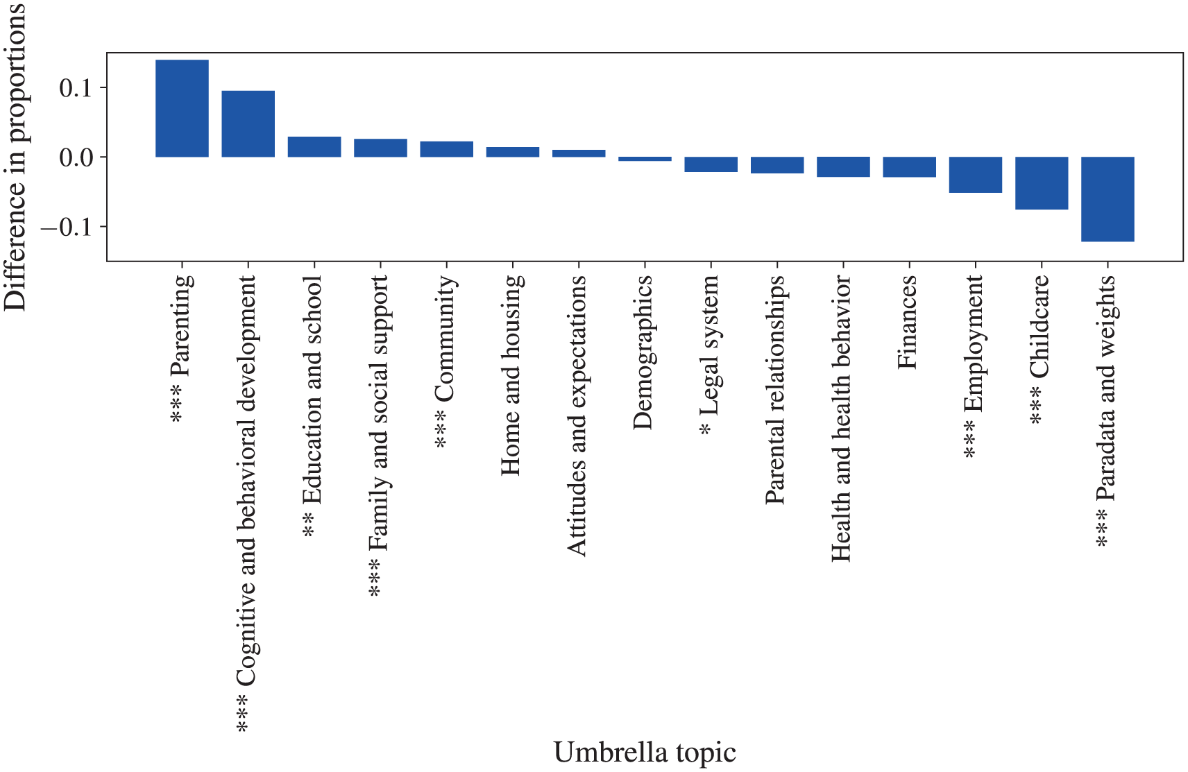
Proportion of LIME-identified variables by umbrella topic relative to entire survey.

Figure 3.

Ratio of umbrella topics in LIME-identified variables relative to entire survey.

Variables relating to parenting occur most frequently in the explanations, about 2.5 times as often as in the overall survey. These capture the parents’ involvement in their children’s lives, in particular interactions with the children, such as whether they read bedtime stories, play outside together, discuss problems, and use physical punishments. This category also includes parental assessments of their children’s behavior, such as how often they watch television and how many mornings a week they eat breakfast. The presence of these variables is consistent with Baker and Stevenson’s (1986) emphasis on the importance of parental involvement: “Parents must do a long series of small things to assist their child toward maximum educational attainment” (p. 165). The fact that these variables occur so frequently in the LIME explanations indicates that the neural network model is identifying them as predictors of GPA.

The other most frequently appearing topic in the LIME explanations, with the highest ratio of occurrences compared with the survey, is the child’s cognitive and behavioral development. Most of these variables relate to the child’s behavior, such as whether they argue a lot, have temper tantrums, tease other children, and have difficulty concentrating in class. Prior work using these data has found that these types of behaviors are associated with poor cognitive development in middle childhood (Turney and McLanahan 2015), and these results indicate that these variables can also predict high school performance.

Variables pertaining to education and the school also appear frequently in the explanations. These include the child’s responses as well as parental and teacher assessments. This is consistent with prior work that has identified the school context as an important predictor of academic performance (Alexander and Eckland 1975). Variables related to the family, social support, and the community also occur significantly more frequently in the explanations than in the survey, suggesting the importance of considering social structures and contexts beyond the parent-child relationship and the school.

Looking at the least frequent variables, it is notable that demographic variables occur only nine times; although these variables are the cornerstone of most sociological analyses, it appears that fine-grained behavioral data may be more useful for prediction. Variables associated with health and health care and the legal system, predominantly relating to the father’s incarceration, do appear in some explanations but occur less frequently than expected. Although prior work has identified these factors to be important determinants of children’s educational outcomes (e.g., Branigan 2017; Haskins 2014), they appear to only be predictive in a small number of cases. Variables relating to parental employment and childcare are far less frequent than in the survey, along with paradata and weights, which is the most frequent category in the survey and largely consists of constructed variables, the latter suggesting that the model may be making more use of the raw variables than any preengineered features.

Turning to the distribution of variables across survey waves, variables from wave 1 occur significantly more frequently in the explanations than in the survey, with a ratio of 1.5:1. This is consistent with prior findings that early childhood indicators can be predict educational attainment in later life (Alexander, Entwisle, and Horsey 1997; Entwisle et al. 2005). Variables from wave 3, which contributed the largest number of variables to the survey, occur significantly less frequently, although it is unclear why.

Turning to the respondent associated with each variable, I find that the vast majority of variables in the explanations are derived from survey segments corresponding to the mother, father, and primary caregiver. The proportions for mother and father are not statistically different from the overall survey, but the explanations contain significantly more variables associated with the primary caregiver and the teacher; the ratios for both respondent types are above 2:1. The primary caregiver, typically the child’s mother—unless children live with their father or another relative—provides information about parenting, child health, and development that appears to be useful for prediction.¹⁰ The finding that variables from the teacher interviews occur more frequently than expected is consistent with studies showing how the teacher-pupil relationship and the teacher’s assessment of the pupil can help explain differences in academic performance (Alexander, Entwisle, and Thompson 1987; Branigan 2017).

Although LIME reveals nothing about the inner workings of the neural network, its post hoc explanations can provide valuable insights into the predictions of the black-box model (Lipton 2016). The variables identified by LIME are broadly consistent with prior work, suggesting that many existing sociological explanations may have predictive validity. Information about parenting, the child’s behavior and cognitive development, community, family and social support, and the school environment appears to be used by the neural network to predict GPA. Early-childhood indicators and responses from the primary caregiver and teacher are particularly important sources of information. These results show how predictive models can be interpreted to help us identify important predictive factors that may help improve our sociological explanations. In particular, we see that fine-grained behavioral variables tend to occur more frequently in LIME explanations than demographic ones, suggesting that we should pay more attention to the former. Moreover, the large number of variables identified in the explanations suggests that neural networks may be useful for identifying heterogeneity that we cannot see when only using a small number of predictors. Nonetheless, it is critical to add the caveat that we must be aware of the danger of interpreting these results as if they are meaningful explanations, let alone causal ones. It is plausible, and indeed highly likely, that many other variables could have similar predictive power (Mullainathan and Spiess 2017) and that we could tell similar stories about them (Watts 2014). These post hoc explanations are no substitutes for models that aim to carefully estimate the $\hat{β}$ values. Further work is therefore necessary to assess the extent to which the predictive variables used in the neural network and identified by LIME are actually determinants of academic success.

Conclusions

The FFC presented a valuable opportunity to examine how black-box machine-learning methods perform at predicting outcomes of sociological interest. The results of my analysis show that neural networks can perform reasonably well at predicting high school GPA but that they do not perform particularly better than more conventional classes of models. I encourage others to build on this foundation by exploring whether other types of neural network architectures are better suited to such tasks. Predictive performance aside, the variables identified by LIME are consistent with prior literature, suggesting that existing sociological explanations of high school GPA, and academic success more generally, have some predictive power. Moreover, this demonstrates that the model was able to sift through thousands of features and learn to use those that had been previously identified in the literature. Notwithstanding the concerns raised by Mullainathan and Spiess (2017), the results suggest that machine learning can provide a valuable complement to more traditional approaches, giving us a data-driven approach to inductively identify important variables. Examination of how these findings can contribute to sociological explanations requires further research to qualitatively study the trajectories of individual children and to explore causal mechanisms by more robustly by estimating $\hat{β}$ values. Although my results are not the best of the entrants to the FFC, I hope to have demonstrated why black-box modeling approaches such as neural networks deserve more attention from sociologists, particularly as they are becoming more amenable to interpretation.¹¹

There are two other important implications of this study. First, despite the attempts to prevent overfitting, there are still substantial differences in model performance across the training, validation, and held-out data sets. Not only does this illustrate the difficulty of constructing models that can generalize out-of-sample, but it also casts doubt on the validity of any results that are only reported in-sample, reinforcing Watts’s (2014) emphasis on the importance of out-of-sample testing. Second, as machine learning becomes more frequently adopted by sociologists, it is important to recognize the nuances of the distinction between explanatory and predictive models, to identify when either approach should be used and when we are able to fruitfully combine them (Mullainathan and Spiess 2017). Overall, I hope that this article highlights the need to reconcile both predictive and explanatory modes of analysis to advance social scientific inquiry. Mass collaboration efforts such as the FFC provide a valuable opportunity to push us toward this goal by simultaneously advancing both our ability to predict social outcomes and to explain the social world.

Supplemental Material

davidson_supplemental_information – Supplemental material for Black-box Models and Sociological Explanations: Predicting High School Grade Point Average Using Neural Networks

Supplemental material, davidson_supplemental_information for Black-box Models and Sociological Explanations: Predicting High School Grade Point Average Using Neural Networks by Thomas Davidson in Socius

Supplemental Material

SRD-17-0112 – Supplemental material for Black-box Models and Sociological Explanations: Predicting High School Grade Point Average Using Neural Networks

Supplemental material, SRD-17-0112 for Black-box Models and Sociological Explanations: Predicting High School Grade Point Average Using Neural Networks by Thomas Davidson in Socius

Footnotes

Acknowledgements

I would like to thank George Berry, Filiz Garip, Michael Macy, Mario Molina, Emily Parker, Tony Sirianni, the participants in the FFC Scientific Workshop held at Princeton University, members of the Social Dynamics Laboratory at Cornell University, the organizers of the FFC, and the Socius reviewers for their comments and suggestions. All errors and omissions are my own. I also want to express my gratitude to the other participants for the help they provided on the FFC forum and for open-sourcing their submissions and other useful resources. The analyses were conducted using the Python programming language. Specific packages are cited where relevant in the text. All of the code to reproduce the analysis and the results can be found at .

Funding

The author(s) disclosed receipt of the following financial support for the research, authorship, and/or publication of this article: Funding for the Fragile Families and Child Wellbeing Study was provided by the Eunice Kennedy Shriver National Institute of Child Health and Human Development through grants R01HD36916, R01HD39135, and R01HD40421 and by a consortium of private foundations, including the Robert Wood Johnson Foundation. Funding for the FFC was provided by the Russell Sage Foundation.

ORCID iD

Thomas Davidson

Supplemental Material

Supplemental material for this article is available with the manuscript on the Socius website.

1

Cross-validation and out-of-sample validation is the norm in computer science and the nascent field of data science but has been neglected by sociologists, despite being known in the field at least since the early 1990s ().

2

See for an overview of neural network models and some major scientific breakthroughs that have been achieved using them.

3

See the FFC blog post on why GPA was selected: .

4

See the Supplemental Information for a discussion of the problems associated with estimating linear regressions using high-dimensional data.

5

By default, only the best performing model is stored after the grid search, so the models needed to be recomputed.

6

I experimented with different values but found that for values higher than five, the algorithm often failed to converge.

7

also proposed a method to find the subset of features that best explain a range of different observations, providing a global approximation, but given that most of the features occur only once, it will be unlikely to find a better solution than inspecting the results and identifying features that recur with high frequency.

8

I was unable to obtain metadata for six of the variables that occurred in these explanations: hv3c_c3, hv3r10a7, hv3cwtalone, hv4cflag, hv4agemos, and hv4food_exp.

9

All figures hereafter were produced using Matplotlib ().

10

See “Introduction to the Fragile Families Public Use Data” for more information about the surveys and the role of the primary caregiver: .

11

See for an excellent and prescient discussion of the potential for these models in the social sciences.

Author Biography

Thomas Davidson is a PhD candidate in the Department of Sociology at Cornell University. His research applies computational methods including natural language processing, machine learning, and social network analysis to the study of politics and culture. His dissertation focuses on social media and contentious politics in the UK. His work has appeared in Social Forces, Mobilization, and ICWSM.

References

Abadi

Martín

Agarwal

Ashish

Barham

Paul

Brevdo

Eugene

Chen

Zhifeng

Citro

Craig

Corrado

Greg S.

et al. 2016. “TensorFlow: Large-scale Machine Learning on Heterogeneous Distributed Systems.” Retrieved November 26, 2018 (https://arxiv.org/abs/1603.04467).

Alexander

Karl L.

Eckland

Bruce K.

1975. “Contextual Effects in the High School Attainment Process.” American Sociological Review 40(3):402–16.

Alexander

Karl L.

Entwisle

Doris R.

Horsey

Carrie S.

1997. “From First Grade Forward: Early Foundations of High School Dropout.” Sociology of Education 70(2):87–107.

Alexander

Karl L.

Entwisle

Doris R.

Thompson

Maxine S.

1987. “School Performance, Status Relations, and the Structure of Sentiment: Bringing the Teacher Back In.” American Sociological Review 52(5):665–82.

Astone

Nan Marie

McLanahan

Sara S.

1991. “Family Structure, Parental Practices and High School Completion.” American Sociological Review 56(3):309–20.

Athey

Susan

. 2017. “Beyond Prediction: Using Big Data for Policy Problems.” Science 355(6324):483–85.

Attewell

Paul

. 2001. “The Winner-take-all High School: Organizational Adaptations to Educational Stratification.” Sociology of Education 74(4):267–96.

Baker

David P.

Stevenson

David L.

1986. “Mothers’ Strategies for Children’s School Achievement: Managing the Transition to High School.” Sociology of Education 59(3):156–66.

Branigan

Amelia R.

2017. “(How) Does Obesity Harm Academic Performance? Stratification at the Intersection of Race, Sex, and Body Size in Elementary and High School.” Sociology of Education 90(1):25–46.

10.

Camstra

Astrea

Boomsma

Anne

. 1992. “Cross-validation in Regression and Covariance Structure Analysis: An Overview.” Sociological Methods & Research 21(1):89–115.

11.

Caraway

Kirsten

Tucker

Carolyn M.

Reinke

Wendy M.

Hall

Charles

. 2003. “Self-efficacy, Goal Orientation, and Fear of Failure as Predictors of School Engagement in High School Students.” Psychology in the Schools 40(4):417–27.

12.

Cavanagh

Shannon E.

Schiller

Kathryn S.

Riegle-Crumb

Catherine

. 2006. “Marital Transitions, Parenting, and Schooling: Exploring the Link between Family-structure History and Adolescents’ Academic Status.” Sociology of Education 79(4):329–54.

13.

Chollet

François.

2015. “Keras.” 2015. Retrieved November 26, 2018 (https://github.com/fchollet/keras).

14.

Cybenko

George

. 1989. “Approximation by Superpositions of a Sigmoidal Function.” Mathematics of Control, Signals, and Systems 2(4):303–14.

15.

Duckworth

Angela L.

Seligman

Martin E. P.

2005. “Self-discipline Outdoes IQ in Predicting Academic Performance of Adolescents.” Psychological Science 16(12):939–44.

16.

Entwisle

Doris R.

Alexander

Karl L.

Olson

Linda Steffel

. 2005. “First Grade and Educational Attainment by Age 22: A New Story.” American Journal of Sociology 110(5):1458–1502.

17.

Foster

Holly

Hagan

John

. 2009. “The Mass Incarceration of Parents in America: Issues of Race/Ethnicity, Collateral Damage to Children, and Prisoner Reentry.” Annals of the American Academy of Political and Social Science 623(1):179–94.

18.

Garson

G. David

. 1998. Neural Networks: An Introductory Guide for Social Scientists. Thousand Oaks, CA: Sage.

19.

Goh

A.T.C.

1995. “Back-propagation Neural Networks for Modeling Complex Systems.” Artificial Intelligence in Engineering 9(3):143–51.

20.

Haskins

Anna

. 2014. “Unintended Consequences: Effects of Paternal Incarceration on Child School Readiness and Later Special Education Placement.” Sociological Science 1:141–58.

21.

Hedström

Peter

Swedberg

Richard

. 1998. “Social Mechanisms: An Introductory Essay.” Pp. 1–31 in Social Mechanisms: An Analytical Approach to Social Theory, edited by Hedström

Peter

Swedberg

Richard

. New York: Cambridge University Press.

22.

Hinton

Geoffrey E.

1992. “How Neural Networks Learn from Experience.” Scientific American 267(3):144–51.

23.

Hofman

Jake M.

Sharma

Amit

Watts

Duncan J.

2017. “Prediction and Explanation in Social Systems.” Science 355(6324):486–88.

24.

Hornik

Kurt

Stinchcombe

Maxwell

White

Halbert

. 1989. “Multilayer Feedforward Networks Are Universal Approximators.” Neural Networks 2(5):359–66.

25.

Hunter

John D.

2007. “Matplotlib: A 2D Graphics Environment.” Computing in Science & Engineering 9(3):90–95.

26.

Kingma

Diederik P.

Jimmy Lei

. 2015. “Adam: A Method for Stochastic Optimization.” Pp. 1–15 in Proceedings of the International Conference on Learning Representations (ICLR). arXiv:1412.6980v9

27.

Krizhevsky

Alex

Sutskever

Ilya

Hinton

Geoffrey E.

2012. “Imagenet Classification with Deep Convolutional Neural Networks.” Pp. 1097–1105 in Advances in Neural Information Processing Systems. Retrieved November 26, 2018 (http://papers.nips.cc/paper/4824-imagenet-classification-with-deep-convolutional-neural-networks.pdf).

28.

Kuan

Chung-Ming

White

Halbert

. 1994. “Artificial Neural Networks: An Econometric Perspective.” Econometric Reviews 13(1):1–91.

29.

LeCun

Yann

Bengio

Yoshua

Hinton

Geoffrey

. 2015. “Deep Learning.” Nature 521(7553):436–44.

30.

Lin

Henry W.

Tegmark

Max

. 2016. “Why Does Deep and Cheap Learning Work So Well? ” Retrieved November 26, 2018 (https://arxiv.org/abs/1608.08225).

31.

Lipton

Zachary C.

2016. “The Mythos of Model Interpretability.” In Workshop on Human Interpretability in Machine Learning. Retrieved November 26, 2018 (https://arxiv.org/pdf/1606.03490.pdf).

32.

Lundberg

Scott M.

Lee

Su-In

. 2017. “A Unified Approach to Interpreting Model Predictions.” Pp. 4768–77 in Advances in Neural Information Processing Systems. Retrieved November 26, 2018 (https://papers.nips.cc/paper/7062-a-unified-approach-to-interpreting-model-predictions.pdf).

33.

McKinney

Wes

. 2013. Python for Data Analysis: Data Wrangling with Pandas, NumPy, and IPython. Beijing, China: O’Reilly.

34.

Mounts

Nina S.

Steinberg

Laurence

. 1995. “An Ecological Analysis of Peer Influence on Adolescent Grade Point Average and Drug Use.” Developmental Psychology 31(6):915–22.

35.

Mullainathan

Sendhil

Spiess

Jann

. 2017. “Machine Learning: An Applied Econometric Approach.” Journal of Economic Perspectives 31(2):87–106.

36.

Nair

Vinod

Hinton

Geoffrey E.

2010. “Rectified Linear Units Improve Restricted Boltzmann Machines.” Pp. 807–814 in Proceedings of the 27th International Conference on Machine Learning (ICML-10). Retrieved November 26, 2018 (http://machinelearning.wustl.edu/mlpapers/paper_files/icml2010_NairH10.pdf).

37.

Olden

Julian D.

Jackson

Donald A.

2002. “Illuminating the ‘Black Box’: A Randomization Approach for Understanding Variable Contributions in Artificial Neural Networks.” Ecological Modelling 154(1):135–50.

38.

Pedregosa

Fabian

Varoquaux

Gaël

Gramfort

Alexandre

Michel

Vincent

Thirion

Bertrand

Grisel

Olivier

Blondel

Mathieu

Prettenhofer

Peter

Weiss

Ron

Dubourg

Vincent

Vanderplas

Jake

Passos

Alexandre

Cournapeau

David

Brucher

Matthieu

Perrot

Matthieu

Duchesnay

Édouard

. 2011. “Scikit-Learn: Machine Learning in Python.” Journal of Machine Learning Research 12 (Oct): 2825–30.

39.

Reichman

Nancy E.

Teitler

Julien O.

Garfinkel

Irwin

McLanahan

Sara S.

2001. “Fragile Families: Sample and Design.” Children and Youth Services Review 23(4–5):303–26.

40.

Ribeiro

Marco Tulio

Singh

Sameer

Guestrin

Carlos

. 2016. “‘Why Should I Trust You?’: Explaining the Predictions of Any Classifier.” Pp. in 1135–44 Proceedings of the 22nd ACM SIGKDD International Conference on Knowledge Discovery and Data Mining. New York: Association for Computing Machinery.

41.

Roksa

Josipa

Potter

Daniel

. 2011. “Parenting and Academic Achievement: Intergenerational Transmission of Educational Advantage.” Sociology of Education 84(4):299–321.

42.

Rubinsteyn

Feldman

2016. “Fancyimpute.” Retrieved November 26, 2018 (https://github.com/iskandr/fancyimpute).

43.

Rumbaut

Rubén G.

2005. “Turning Points in the Transition to Adulthood: Determinants of Educational Attainment, Incarceration, and Early Childbearing among Children of Immigrants.” Ethnic and Racial Studies 28(6):1041–86.

44.

Rumelhart

David E.

Hinton

Geoffrey E.

Williams

Ronald J.

1986. “Learning Representations by Back-propagating Errors.” Nature 323:533–36.

45.

Salganik

Matthew J.

Lundberg

Ian

Kindel

Alexander T.

McLanahan

Sara

. 2019. “Introduction to the Special Collection on the Fragile Families Challenge.” Socius 5. doi:10.1177/2378023119871580.

46.

Srivastava

Nitish

Hinton

Geoffrey E.

Krizhevsky

Alex

Sutskever

Ilya

Salakhutdinov

Ruslan

. 2014. “Dropout: A Simple Way to Prevent Neural Networks from Overfitting.” Journal of Machine Learning Research 15(1):1929–58.

47.

Turco

Catherine J.

Zuckerman

Ezra W.

2017. “Verstehen for Sociology: Comment on Watts.” American Journal of Sociology 122(4):1272–91.

48.

Turney

Kristin

McLanahan

Sara

. 2015. “The Academic Consequences of Early Childhood Problem Behaviors.” Social Science Research 54:131–45.

49.

Tzeng

F.-Y.

K.-L.

2005. “Opening the Black Box—Data Driven Visualization of Neural Networks.” Pp. 383–90 in Visualization, 2005. VIS 05. IEEE. Retrieved November 26, 2018 (https://doi.org/10.1109/VISUAL.2005.1532820).

50.

Wang

Ming-Te

Sheikh-Khalil

Salam

. 2014. “Does Parental Involvement Matter for Student Achievement and Mental Health in High School?” Child Development 85(2):610–25.

51.

Watts

Duncan J.

2014. “Common Sense and Sociological Explanations.” American Journal of Sociology 120(2):313–51.

52.

Wolters

Christopher A.

1999. “The Relation between High School Students’ Motivational Regulation and Their Use of Learning Strategies, Effort, and Classroom Performance.” Learning and Individual Differences 11(3):281–99.

Supplementary Material

Please find the following supplemental material available below.

For Open Access articles published under a Creative Commons License, all supplemental material carries the same license as the article it is associated with.

For non-Open Access articles published, all supplemental material carries a non-exclusive license, and permission requests for re-use of supplemental material or any part of supplemental material shall be sent directly to the copyright owner as specified in the copyright notice associated with the article.

0.75 MB

0.00 MB

2.02 MB

Black-Box Models and Sociological Explanations: Predicting High School Grade Point Average Using Neural Networks

Abstract

Keywords

Background

Prediction and Sociological Explanations

Neural Networks and Deep Learning

Predicting High School GPA

Methods

Data Cleaning and Transformations

Constructing Neural Network Models

Cross-validation and Model Estimation

Results

Comparing Network Architectures

Interpreting Black-box Models

Conclusions

Supplemental Material

davidson_supplemental_information – Supplemental material for Black-box Models and Sociological Explanations: Predicting High School Grade Point Average Using Neural Networks

Supplemental Material

SRD-17-0112 – Supplemental material for Black-box Models and Sociological Explanations: Predicting High School Grade Point Average Using Neural Networks

Footnotes

Acknowledgements

Funding

ORCID iD

Supplemental Material

1

2

3

4

5

6

7

8

9

10

11

Author Biography

References

Supplementary Material