
Abstract
Despite the tendency for some to view rural life or living close to nature with nostalgia, the unpalatable truth is that rural America is beset with many problems, including lower incomes, higher poverty rates, limited access to well-paying jobs, higher morbidity and mortality rates, inadequate access to health care, and lower educational attainment. In this study, we question whether this palpable rural disadvantage extends to residential energy costs, a subject with serious implications for the well-being of households. Analyses of data spanning two decades show that rural households consistently spend more on residential energy than urban households, although they generally use less. This finding, which indicates the existence of energy cost inequality between rural and urban places, represents a kind of rural tax. Any sustained spikes in costs, which has happened in the past and would likely happen in the future, could portend significant access risks to rural households.
Keywords
Introduction
Rural America has witnessed substantial transformation over the past two centuries. The proportion of Americans residing in rural places dropped from about 84.5 percent in 1850 to slightly less than 20 percent in 2010 (Gibson 2015). This transformation is driven partly by structural changes in the American economy and rural locations’ general disadvantage relative to other places (Lobao 1990). While rural life or living close to nature is often viewed with nostalgia by some, the unpalatable truth is that rural America is confronted by several social problems and disadvantages. Researchers have over the years documented rural-urban disparities in many markers of well-being, with residents of rural places faring considerably worse (Albrecht 2012; Beaulieu 2002; Flora and Flora 2008; Larson and Hill 2005; Lichter and Costanzo 1987; Thiede, Lichter, and Slack 2018; Tickamyer and Duncan 1990; Waity 2016; Whitener, Duncan, and Weber 2002). These studies show that America’s opportunity structure differs by place, with rural locations possessing comparatively limited opportunities.
In this study, we examine the extent to which the prevailing multifaceted rural disadvantage extends to residential energy costs. This work is an effort to extend the frontiers of inequality research in sociology to an area that has received little or no attention. We draw on a political economy perspective on place-based inequality (i.e., the growth machine theory) to empirically examine the extent to which residential energy costs (what we refer to as energetic pain) vary by residence along the rural-urban continuum while holding constant the impacts of consumption and many other variables. We focus on cost because of its implication for access. In a developed nation such as the United States, which has a well-developed energy exploitation and distribution infrastructure, one of the most effective ways to examine access to energy, a hard to substitute resource, is exploring its costs to the end user. There is evidence that lower-income households often respond to increases in energy costs by cutting back on the consumption of energy and other essential provisions (Child Health Impact Working Group 2007; Dillman, Rosa, and Dillman 1983).
While several sociological studies have addressed the subject of energy (see Adua 2010; Adua and Sharp 2011; Cramer et al. 1985; Dillman et al. 1983; Hackett and Lutzenhiser 1991; Lutzenhiser 1993, 1994; Lutzenhiser and Hackett 1993; Lutzenhiser, Harris, and Olsen 2002; York 2017; York and McGee 2017), there are hardly any that have examined energy costs and expenditure patterns at the household level. Sociologists have largely ceded this aspect of energy-related research to economists and other policy-oriented researchers, although this subject has serious implications for the well-being of households and individuals. In addition to addressing this significant limitation in the broader sociological literature, our analysis of rural-urban inequality in energy costs contributes to a long line of research in rural sociology highlighting and documenting the persistent and emergent challenges of rural America, often in contrast to urban places (Allen 2002; Brown and Hirschl 1995; Cotter 2002; Flora and Flora 2008; Lobao 2004; Tickamyer and Duncan 1990). Analyzing the position of rural relative to urban America is one of the most enduring aspects of sociological work on spatial inequality in the United States (Brown and Schafft 2011; Hooks, Lobao, and Tickamyer 2016; Lobao 2004; Lobao and Saenz 2002). By focusing on this understudied dimension of place-based inequality, energy costs, our ultimate goal is to offer some thoughts about its implications for households’ access to residential energy and the social mobility of rural places and people. It also represents a unique take on the broader sociological work on social inequality, a defining character of the discipline (see e.g., Brailsford et al. 2018; Liao 2016; Lu 2017; Moller, Alderson, and Nielsen 2009; Nau 2013; Reardon and Bischoff 2011).
We address our research question by analyzing four waves of the residential energy consumption surveys (RECS), which are cross-sectional surveys conducted quadrennially by the Energy Information Administration (EIA) of the US Department of Energy. The surveys collect information on households’ energy expenditures, the primary dependent variable of interest, and many other variables. Detailed description of the data and the measures used are provided later in the article.
In the sections that follow, we first briefly discuss the energy and society nexus. Next, we discuss the political economy perspective on spatial inequality, which we draw on to guide our analysis, zeroing in on the growth machine theory. This is followed with a discussion of the data, methods, and results. Based on our analysis of the data, we conclude that rural households, on average, experience higher residential energy costs than their urban counterparts in spite of the fact that they (i.e. rural households) use less energy.
Society and Energy
Energy plays a significant role in conditioning how societies and social institutions are structured. The availability of energy, the ability to transform it into usable forms, along with how it is put into use help determine lifestyles, patterns of communication, and features of social structure and change (Lutzenhiser 1993; Rosa, Machlis, and Keating 1988). Underscoring the importance of energy in the functioning of society, Cottrell (1955:2) observed that “the energy available to man limits what he can do and influences what he will do.”
Energy, in essence, represents a central input in social metabolism at both the micro and macro levels of society. In the United States’s residential sector, energy is used primarily for such essential things as lighting, space heating and cooling, water heating, cooking, and laundry.
While the longstanding positive relationship between energy consumption and economic development has attenuated somewhat since the 1950s (Mazur and Rosa 1974), households in the United States and elsewhere still need adequate and moderately priced supplies of energy to maintain healthy living conditions for their members. As noted in the introduction, exorbitant energy prices will most certainly pose dire access challenges to low-income families, possibly forcing them to make tradeoffs between different areas of household consumption.
We will be remiss if we fail to point out that the weakened relationship between energy consumption and economic development is in fact not indicative of the diminishing importance of energy to society. It is mostly a function of increasing efficiency gains in energy use. For example, an online report issued by the Energy Information Administration of the US Department of Energy shows homes built between 2000 and 2009, although larger by 30 percent, used 21 percent less energy for space heating on average than older homes. 1 The report attributes this reduction in energy consumption to the use of more efficient heating equipment and building shells that now conform to stricter energy efficiency codes. This study thus addresses a subject that is of great importance to sociology and society, rural-urban inequalities in energy costs and access risks.
Political Economy, Place Stratification, and Rural Disadvantage
Systematic social and economic inequalities exist among US residential places. Place stratification in the contemporary United States tends to be disadvantageous to rural and inner-city locations (see Albrecht, Albrecht, and Albrecht 2000; Lobao, Hooks, and Tickamyer 2005; Tickamyer and Duncan 1990; Waity 2016). Several sociological perspectives, both micro and macro, have informed research on uneven development and spatial inequality. This study draws on a political economy (PE) perspective, the growth machine theory, to frame energy cost inequality between rural and urban places. The PE perspective is an eclectic sociological approach to the study of uneven development/spatial inequality (Loboa and Hooks 2015).
The broader PE framework emphasizes the role of economic structure, institutional processes and arrangements, and actions of the state in determining development, or place stratification (see Lobao et al. 2008; Lobao and Hooks 2015; Tickamyer 2000). The framework recognizes that localities do compete with each other to maintain or elevate their relative positions in the place-based stratification system (Logan 1978; Logan and Molotch 1987; Molotch 1993), with the factors identified previously (economic structure, institutional processes, and the state) playing decisive roles in determining the resulting pecking order. Advocating for this framework, Logan (1978:409) has argued that in “conflicts over boundaries, constitutional powers, allocation of public resources, taxation policies, land use controls, etc., places compete for development outcomes which would maintain or improve their relative positions in the hierarchy of places.” Indeed, the local economic development literature is replete with studies showing localities of all sizes competing for businesses and other development projects (Friedland and Palmer 1984; Lobao and Adua 2011; Lobao, Adua, and Hooks 2014; Reese and Rosenfeld 2002). Pointing out the primary source of place stratification while discounting a central argument of the human ecology perspective, Logan and Molotch (1987:45) observe that places achieve their attributes “through social action, rather than through the qualities inherent in a piece of land.”
In essence, the PE framework posits that spatial differentiation is a stratification system that reflects power relations between places. Interplace competition over valued social goods and opportunities are driven largely by the twin goals of growth and status maintenance or elevation. Molotch’s (1976) growth machine (GM) theory, a well-known PE perspective on local governance, provides important insights concerning why and how localities engage in competition with each other. The growth imperative, which is essential for any given locality to maintain or improve its position in the place-based stratification system, is the primary driver of interplace competition. In line with the broader framework of the PE perspective, the GM theory asserts that the primary goal of US localities is growth (Logan and Molotch 1987; Molotch 1976). Logan and Molotch (1987:13) have argued that this “growth ethic pervades in virtually all aspects of local life, including the political system, the agenda for economic development, and even cultural organizations like baseball teams and museums.”
To be able to engage in competition or pursue growth, places, which are inherently inanimate, must have the capacity to act independently as individuals must often do, that is, they must possess agency. An important contribution of the GM theory to the PE framework is that it suggests how places come to possess agency. The GM perspective argues that a coalition of local pro-growth actors, collectively referred to as the growth machine, provide the agency with which localities act. This coalition includes such local power elites as real estate developers/owners, builders, other local businesses (e.g., the local media and utilities), and local politicians staking their careers on growth (Logan and Crowder 2002; Logan and Molotch 1987; Logan, Whaley, and Crowder 1997; Molotch 1976; Vogel and Swanson 1989). A case study by Rudel (1989) also identified farmers as important members of the growth machine coalition in the rural-urban fringe. According to Logan and co-authors (1997), the urban future is shaped by the influence of this pro-growth coalition (i.e., GM), which incidentally dominates local politics in places across the United States.
Constituent members of the GM work for growth by harnessing the legislative, fiscal, and legitimating powers of local governments to protect and pursue their interests, including land-use intensification (Jonas and Wilson 1999). The coalition molds local policy (Logan et al. 1997), often by sponsoring or capturing politicians amenable to the agenda of growth. GM coalitions also pursue growth by often scuttling or overcoming any emergent anti-growth politics in their areas of influence (Vogel and Swanson 1989; Warner and Molotch 2000). While what motivates the GM coalition to act is its dogged interest in the growth and dynamism of the local economy, any resulting growth invariably serves localities’ interests in maintaining or improving their positions in the hierarchy of places, with the accruing social benefits dripping down to individuals and households.
The key to understanding how this affects place-based inequality is that interplace competition, in the first place, is unequal. In terms of the factors identified as playing decisive roles in determining place stratification—economic structure, institutional processes and capacity, and state influence—localities are not equally endowed. Locations with greater advantage in these factors, which will tend to be more urban, are better positioned to win this competition, which inevitably benefits their inhabitants (Logan 1978). Empirical studies show, for instance, that localities with greater institutional capacity and broader revenue bases are able to formulate and implement a wider variety of policies, including those aimed at boosting local economic growth, than those with limited capacity (Adua and Lobao forthcoming; Lobao et al. 2014).
More specifically connected with this study, it is reasonable to anticipate that urban places can use their combination of superior economic, institutional, and political leverage to attract and/or maintain utility service providers at better rates, which will inevitably benefit their inhabitants. One practical mechanism through which the better resourced urban places can achieve this is the use of lucrative fiscal and other incentive packages to attract corporations, including utility providers. The specific incentives often used include tax abatements and deferral, grants or loans, the provision of appropriate infrastructure, technical assistance, job training grants, hiring assistance, and subsidized business loans (Donahue 1997; Lobao et al. 2014; Reese, Larnell, and Sands 2010; Reese and Rosenfeld 2004; Schram 1999). These incentives drive down what business leaders generally refer to as the “cost of doing business,” which will include production and distribution costs. For utility firms, both production and distribution costs play important roles in the setting of rates for the final consumer, including families and households. This makes it more likely that utility service providers can set up shop in urban places and offer competitive rates to users of their services. Urban places, given their comparatively better institutional and bureaucratic capacities, are also better positioned to craft, implement, monitor, and experiment with a wider variety of policies, including ones that may be attractive to businesses, than rural places (for discussions on the relationship between high capacity and policy-related performance of places, see Clingermayer and Feiock 2001; Jenkins, Leicht, and Wendt 2006; Soule and Zylan 1997; Warner 2006). Utilities in urban places are more than likely to compete with rivals attracted by the incentives, policies, and other advantages these places offer, the consequence of which could be lower rates for consumers. The arguments presented here cannot be said of rural locations, which are generally less leveraged.
The GM constituent members’ penchant for growth, in a perverse fashion, provides an additional reason to, on the contrary, expect higher utility rates in rural locales. Unlike other GM member-entities, which can continually whip up consumption among current and future customers ad infinitum, utilities are placed in the contradictory position of needing to promote greater efficiency in utility utilization among customers and expanding and achieving greater profitability. In fact, there is longstanding evidence of utility firms, especially electric power providers, offering incentive programs to households and families to curtail consumption (Relf, Baatz, and Nowak 2017; Stern et al. 1986). All else being the same, efficiency improvement often means reduced consumption of the commodity that utility firms sell and want to sell. To grow and expand, utilities then often have to acquire new customers, which sometimes causes them “to penetrate deep into the hinterlands, inefficiently extending lines to areas that are extremely costly to service” (Logan and Molotch 1987:74). This is most certainly more applicable to rural utilities than those based in urban places. For example, in 2005, the distribution cost of electric co-ops, which largely serve rural populations, was more than twice as much as the distribution cost of investor-owned utilities, which generally operate in high-density places (Cooper 2008). All or part of utility distribution costs inevitably get passed on to the final consumer. The point here is that the quest for growth often blinds utilities from considering more cost-effective ways of providing services to residents of open country places.
We observe that economists simply attribute the kind of urban advantage suggested in the above discussion to agglomeration economies of scale, the economic benefits associated with having a heavy concentration of people and organizations in a given geographic location. However, this does not nullify the argument of the GM theory. Our article draws on an alternative explanation (i.e., sociological) of urban advantage. The concentration of people and organizations in one location and not the other does not occur by accident or due to the inherent qualities of a piece of land: Agglomeration and the associated economies of scale are created and sustained by interplace competition for people and organizations (Logan 1978; Logan and Molotch 1987; Reese and Rosenfeld 2002). For example, there is currently an ongoing fierce battle among several large American cities to attract Amazon’s second headquarters. Not surprisingly, there are no rural communities or midsize cities in this battle. It is a battle of titans only.
The foregoing discussion strongly suggests place-based stratification will most likely favor urban places, with the attendant distribution of social goods and opportunities to the members of society (individuals and households) likely following a similar pattern. Empirical evidence from the extant literature supports this predicted relationship (Albrecht 2012; Beaulieu 2002; Byun, Meece, and Irvin 2012; Eberhardt and Pamuk 2004; Flora and Flora 2008; Larson and Hill 2005; Partridge and Rickman 2008a, 2008b; Snyder and McLaughlin 2004; Thiede et al. 2018; Tickamyer and Duncan 1990; Waity 2016; Weber, Duncan, and Whitener 2001). To what extent, though, will this rural disadvantage extend to residential energy costs? Based on the discussion presented previously, we expect rural locations, given their relative general disadvantage, to be associated with higher residential energy costs than urban locations. Rural places may not have the economic, political, and institutional clout to extract rate concessions from utility firms.
Previous Research on Residential Location and Energy
The extant literature on the subject of energy is almost totally bereft of studies systematically examining rural-urban disparities in residential energy costs. One exception is a study by William Hawk (2013), which reported mixed findings on the subject: It shows rural residents spending more on electricity and fuel oil than urban residents and less on natural gas. The main limitation of Hawk’s study is that it does not control for the impacts of variables that mediate the relationship between residential location and energy expenditures (costs), such as consumption level, household size, housing characteristics, region, and many others. For instance, there is evidence that household size is an important demographic driver of residential energy consumption (Muratori 2013; O’Neil and Chen 2002), which in turn is a major determinant of energy-related expenditures.
We point out and briefly discuss studies examining the relationship between residential location and energy consumption. This is because residential energy consumption is a major determinant of energy costs. There are several studies documenting rural-urban differences in residential energy consumption (Adua and Sharp 2011; Grier 1977; Heberlein, Fuguitt, and Rathbun 1985; Meyer 2013; Muratori 2013; Parshall et al. 2010; Zelinsky and Sly 1981). The studies noted above report generally mixed relationships between residential location (rural vs. urban) and residential energy consumption. On the one hand, several of these studies report a positive relationship between urban residence and energy consumption (Grier 1977; Zelinsky and Sly 1981). Another set of the studies, on the other hand, reports a positive relationship between rural residence and residential energy consumption (Heberlein et al. 1985; Muratori 2013). Muratori (2013) estimates that households in rural places consume 10 percent more energy even though they are generally more energy efficient. While the exact sources of these conflicting findings cannot be definitively determined from the current literature, it is nevertheless useful to consider household energy consumption as a potential driver of residential energy costs. Thus, we model residential energy consumption as one of our main predictors, treating it as a statistical control and important mediator of the relationship between residential location and residential energy costs.
Data and Methods
The unit of analysis in this study is the household. The data used come from the 1993 (N = 7,111), 1997 (N = 5,900), 2005 (N = 4,382), and 2009 (N = 12,083) waves of the Residential Energy Consumption Surveys (RECS). The RECS are area probability cross-sectional surveys conducted quadrennially by the Energy Information Administration (EIA) of the US Department of Energy. The first wave of the RECS was conducted in 1978. The surveys collect environmental and energy-related data from occupied US housing units. The RECS are authorized by the Federal Energy Administration Act of 1974 (PL 93-275) as amended and the 1992 Energy Policy Act (EIA 2013).
Data collection involved the use of trained professional interviewers to administer standardized questionnaires, which helped ensure the accuracy of the data. Questionnaires were administered to household members knowledgeable about energy use within the home, rental agents for sampled housing units where all or part of energy costs are included in the rent, and respondents’ energy suppliers. Interviewers also physically measured and recorded dimensions of sampled housing units, providing valuable information on home size and other related physical characteristics.
Several more strategies were employed to further ensure the accuracy of the data. First, interviewers used help screens or cards to offer respondents standardized definitions or examples. Second, hot-deck imputation 2 was used to fill in missing values (item nonresponse). Third, each data file comes with a sampling weight adjusted for unit nonresponse (outright nonparticipation) and other survey design components. Other strategies included comparing the research subjects’ responses to interviewers’ field notes and recontacting them (the respondents) if any discrepancies are noticed. Additional information about the RECS is available at the website of the EIA (http://www.eia.gov/consumption/residential/index.cfm).
With the goal of modeling data that spread across two decades (the 1990s and 2000s), we selected two contiguous waves of the RECS in each of the decades (1993 and 1997 for the 1990s and 2005 and 2009 for the 2000s). We did this for two reasons. First, because we are unable to conduct pooled analysis of the data, as some of our variables are not measured the same way across the surveys, we thought it practical to limit our analysis to the four most recent waves of the survey. Analyzing additional waves will require more writing space, which does not seem necessary; the four waves we consider are sufficient for answering the research question we posed. Second, two decades is a long enough time period to identify and discern any potential shifts in households’ energy cost patterns.
Dependent Variable: Residential Energy Costs
The main dependent variable in this study is residential energy costs as measured by households’ annual residential energy expenditures. As part of the surveys, households’ monthly energy bills for the various fuels were obtained from their utility suppliers and annualized to create estimates of annual energy expenditures. To construct this variable, we summed households’ expenditures on electricity, natural gas, and fuel oil (see Table 1 for summary statistics). Analyzing these energy expenditures separately will likely lead to misleading results as they (the energy expenditures) are dynamically related to each other. For example, some households may spend significantly more on electricity not simply because they use more of it or have higher costs but because they spend no money on natural gas and/or fuel oil. Many American households do not use natural gas or fuel oil. For our multivariate analysis, we log-transformed this variable due to very wide values range. We have provided summary statistics for annualized household expenditures for each of the energy sources we are focusing on in Table 1.
Measures and Summary Statistics for Households’ Energy Costs, Place of Residence, Energy Consumption, and Other Statistical Control Variables.

These are Taylor linearized standard errors. Taylor linearization corrects for the design characteristics of the sample (area probability sampling). The surveys are not based on simple random samples, for which reason we computed these descriptive statistics using sampling weights included in the data files.
Independent Variables
The primary independent variable in this study is respondents’ place of residence. The main reason why we opted for separate analysis of the data files (rather than pooled cross-sectional analysis) is that place of residence is not measured the same way across all four surveys. While measurement of this variable in the 1993 survey was based on interviewer observation, the 1997 and 2005 surveys measured it by respondents’ self-reports. In the 1993 survey, interviewers were directed to “circle one number below to show the kind of area that the household is in,” with the following response options: city, town, suburbs, and rural or open country. In the 1997 and 2005 surveys, respondents were asked, “Which of the following best describes the location of your home? Do you live in a city, a town, the suburbs, or in a rural area?” For the 2009 survey, respondents’ places of residence were classified as urban or rural based on US Census Bureau codes. In terms of validity of these measures, we note first that they have been used in previous research (see Adua and Sharp 2011). Second, the EIA, which runs the RECS survey program, took several measures to ensure the integrity of the surveys generally and validity of the measures specifically. Summary statistics for the place of residence categories are reported in Table 1.
Another key independent variable in this study is annual residential energy consumption. It is measured with annualized monthly residential consumption figures for electricity, natural gas, and fuel oil, which were obtained directly from responding households’ utility service providers. The figures are made available in British thermal units (BTUs), a measure of the heat content of an energy source. To create a composite measure of residential energy consumption, we summed the BTU measures of the energy types mentioned previously. For our multivariate analysis, we similarly log-transformed this variable due to very wide values range. The fact that these measures are based on actual energy consumption records, to a very large degree, ensures their validity. We expect this variable to majorly mediate the relationship between residential location along the rural-urban continuum and energy costs. Summary statistics for households’ residential energy consumption are also reported in Table 1.
Other predictors included in the analysis are: home size, adequacy of insulation, age of home, heating degree days, cooling degree days, region, annual household income, age of household head, race of household head (race), sex of household head (gender), and household size. Additional information on all these variables, including how each is measured, is shown in Table 1. We include these variables because previous studies show they influence households’ residential energy consumption (see Adua and Sharp 2011; Adua, York, and Schuelke-Leech 2016), which in turn influences households’ residential energy costs. It is likely that these variables will retain residual impacts on residential energy costs, besides their impacts via consumption. As part of our diagnostics, we considered potential interactions between some of these variables (income, race, gender, and number of household members) and residential location along the rural-urban continuum but did not find any consistent patterns across the models.
Model Specification and Estimation
While our primary concern is to consider the extent to which residential location influences energy costs, several other variables are included in the analysis as statistical controls. Diagnostic tests show, however, that a good number of these statistical controls, including residential energy consumption, are causally related to other variables in the model (i.e., they are endogenous to the model). As an example, the diagnostics show that income and residential energy consumption, which we are treating as predictors of residential energy costs, are each explained by residential location along the rural-urban continuum and other variables in the model. An appropriate modeling of the data must account for this observed endogeneity, and in this case, we opted for structural equation modeling (SEM) with observed variables. With SEM, we are able to treat these variables both as explanatory and explained variables, effectively addressing the observed endogeneity. The SEM analytic tool allows us to model the various pathways linking residential energy costs (expenditure patterns) to the independent variables. We used the Mplus statistical software package. The estimator used is MLR, Mplus’s option for maximum likelihood estimation.
The model fitted to the data is represented by the stream of equations shown below this paragraph. It is an observed variables structural equation model (see Bollen 1989). The model comprises seven equations, which correspond to its seven endogenous (dependent) variables. Note that the proposed model includes a reverse-causal link between household size (
Model:


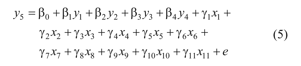

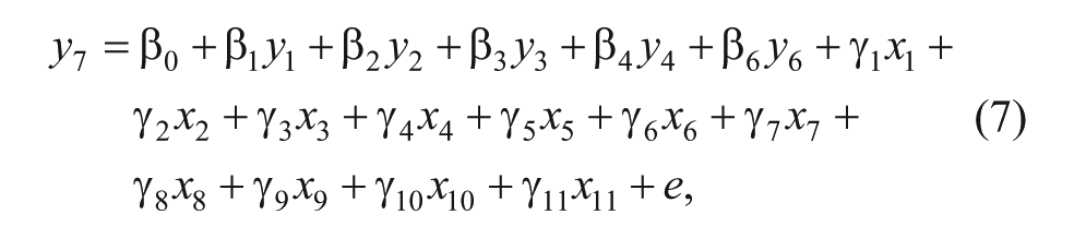
where:
To account for the design effects inherent in the surveys (as they are based on a complex sampling procedure), all models reported in this study are based on weighted analysis of the data. Each data file comes with a weighting variable that adjusts for all the design effects as well as nonresponse.
Results
In this section, we present the results of the study. First, we briefly present bivariate analysis showing the relationship between households’ residential location along the rural-urban continuum and energy consumption and costs. We next present the multivariate models; these are reported in Tables 2 through 5. Before discussing the results of the multivariate models, we will first discuss the associated goodness-of-fit statistics (chi-squares, root mean square of error approximation [RMSEA], and comparative fit index [CFI]).
Structural Equation Model Results: Full Model Results of the Effects of Residential Location and Other Variables on Log Residential Energy Costs, 1993.

Reference category for residential location is city.
Reference category for region is Northeast.
Reference category for race of household head is white.
p < .05. **p < .01. ***p < .001.
Structural Equation Model Results: Full Model Results of the Effects of Residential Location and Other Variables on Log Residential Energy Costs, 1997.
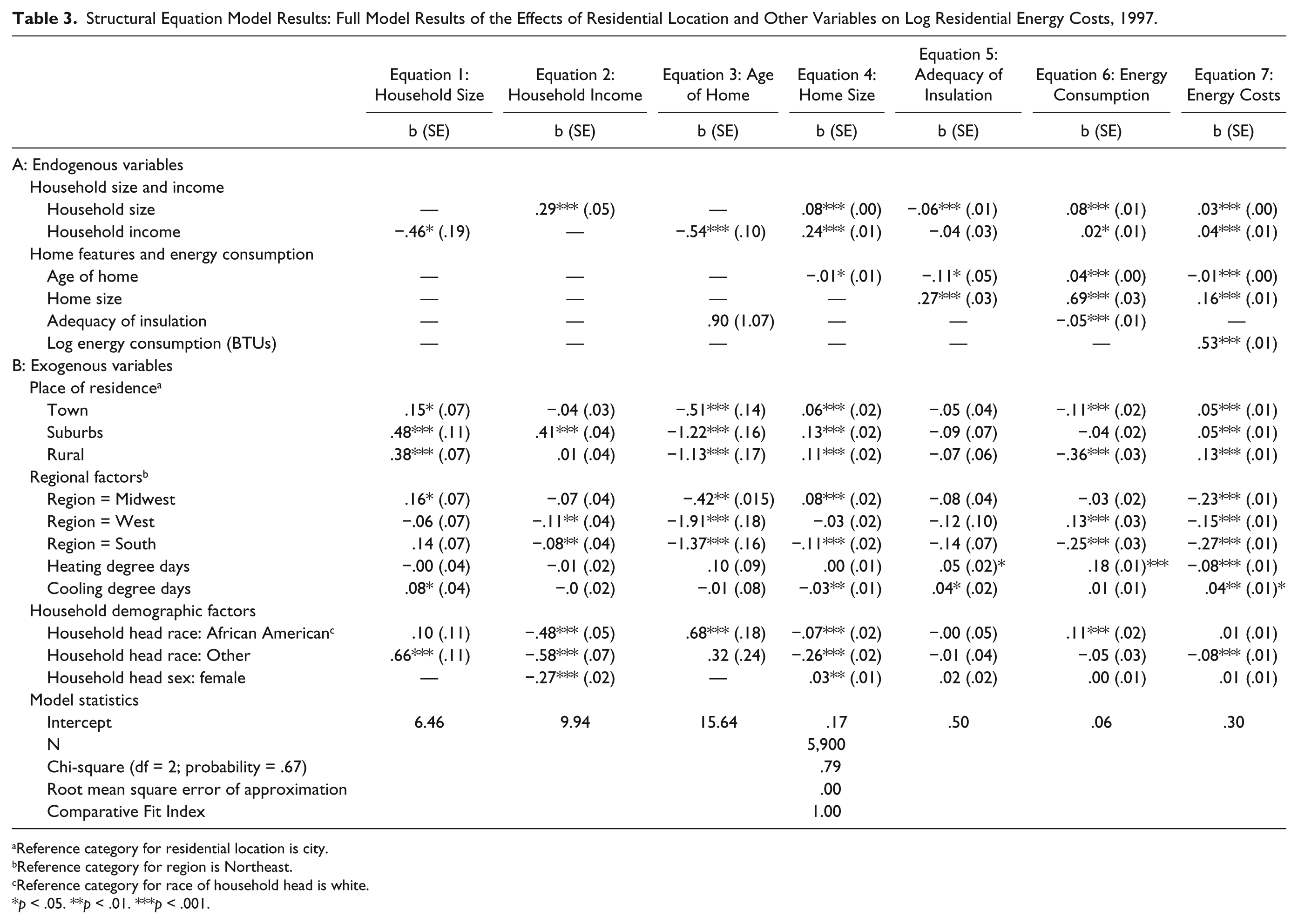
Reference category for residential location is city.
Reference category for region is Northeast.
Reference category for race of household head is white.
p < .05. **p < .01. ***p < .001.
Structural Equation Model Results: Full Model Results of the Effects of Residential Location and other Variables on Log Residential Energy Costs, 2005.

Reference category for residential location is city.
Reference category for region is Northeast.
Reference category for race of household head is white.
p < .05. **p < .01. ***p < .001.
Structural Equation Model Results: Full Model Results of the Effects of Residential Location and other Variables on Log Residential Energy Costs, 2009.

Reference category for residential location is city.
Reference category for region is Northeast.
Reference category for race of household head is white.
p < .05. **p < .01. ***p < .001.
Bivariate Relationships
Across the four cross-sectional data sets analyzed, bivariate results show an interesting mismatch in energy consumption and costs among rural households. Although households residing in rural places use less residential energy in comparison to their urban counterparts, the data suggest they experience higher costs. Rural households consumed about 12,264.5 BTUs, 10,903.2 BTUs, 9,637.3 BTUs, and 7,198.9 BTUs less residential energy than urban households in 1993, 1997, 2005, and 2009, respectively (full results not shown but available on request). On the contrary, however, bivariate analysis of the data (not shown) shows households in rural America spending significantly more on residential energy between 1993 and 2009 than urban households. Based on the GM perspective and the broader literature on spatial inequality, we had anticipated that rural residents will be disadvantaged in terms of energy costs, and this appears to be the case. The next step is examining whether or not this apparent rural tax will persist once we account for the impacts of residential energy consumption and many other relevant variables.
Multivariate Results: Structural Equation Models
Results from fitting the SEM described previously to the four data sets are reported in Tables 2 through 5. Our discussions will center on Equation 7 of the SEM models presented. For each model, Equation 7 has residential energy costs as the dependent (endogenous) variable. While the discussion will focus on the influence of residential location on energy costs, we will offer brief comments on the impacts of some of the statistical control variables. The results pertain to summed household expenditures on electricity, natural gas, and fuel oil. 3
In terms of model fitness, several goodness-of-fit statistics (reported under Model Statistics in Tables 2–5) show reasonably good fits between the proposed model and the data sets. These statistics include: nonsignificant chi-squares (which is indicative of good model-data fit in SEM), RMSEAs of .00 (where an estimate of .08 or less is conventionally considered indicative of a good model-data fit in SEM), and CFIs of 1 (where 1 or closeness to 1 is indicative of good model-data fit in SEM). The across-board nonsignificance of the chi-square statistics, in spite of our rather large sample sizes, provide further indication of the good fit between the model and the data.
Consistent with insights from the political economy perspective on place-based inequality as well as the relevant sociological and related literatures, we find that the prevailing multifaceted rural disadvantage applies to residential energy costs. As shown across all four models, the analysis shows that American households residing in rural places spend significantly more on residential energy than their counterparts in urban places. Controlling for the impacts of several variables associated with energy costs, the analysis shows that households residing in rural places spent 16 percent more on residential energy than households residing in urban places in 1993 (Table 2, Equation 7). What does 16 percent mean in terms of actual costs? Given urban households’ average spending of about $1,133.41 in 1993 (not shown), the 16 percent difference suggests rural households would have spent an estimated $181.35 more on residential energy, that is, about $1,314.8 on average. Four years later, that is, in 1997, the data show rural households remaining relatively disadvantaged in terms of residential energy costs: They spent 13 percent more on residential energy than urban-based households (Table 3, Equation 7). With an average urban residential energy expenditure of $1,177.71 in 1997 (not shown), rural households would have spent an average of about $151.10 more on residential energy than households in urban places.
Although attenuating somewhat over the next several years, the rural-urban disparities in residential energy costs remained statistically significant and quite substantial. In 2005, American households residing in rural places spent about 12 percent more on residential energy than households in urban places (Table 4, Equation 7). In 2009, the difference dropped slightly, with rural households spending 11 percent more on residential energy than their counterparts in urban places (Table 5, Equation 7). Taking the average expenditure of urban households in 2009 into account (i.e., an estimated $1,924.88), this difference comes to an average of about $211.74 more spending by rural households.
The irony of the foregoing finding is that rural households, on average, consume significantly less residential energy than urban households, confirming the pattern suggested in the bivariate results. According to the data, households based in rural places used 44 percent less residential energy in 1993, 36 percent less in 1997, 27 percent less in 2005, and 24 percent less in 2009 (see Tables 2–5 respectively, Equations 6). This is quite intriguing, given that the setting of utility rates in the United States is generally understood to be progressive. Most residential utility customers are placed on the increasing block rate approach to pricing, where the price per unit increases as consumption increases (McNabb 2005, 2016). Our data generally appear to confirm this practice with consumption level driving most of the variability in residential energy costs. The data show that a percentage change in consumption results in 5.4 percent change in cost in 1993, 5.3 percent in 1997, 6.8 percent in 2005, and 6.7 percent in 2009 (Table 2–5, Equations 7). However, it appears the prevailing progressive approach to setting utility rates does not apply to rural households, especially in terms of residential energy. In spite of their relative frugality in residential energy consumption, rural households, according to the data, are saddled with higher energy costs than their urban counterparts. The finding, no doubt, represents a significant financial burden on rural households and portends for them serious residential energy access and social mobility risks.
Turning to the other categories of residential location, we find that residents of towns and suburbs also experienced higher residential energy costs in 1993 and 1997 (Tables 2 and 3). By 2005, however, these differences had disappeared (Table 4). The 2009 measure of residential location has only two categories, rural and urban. What potentially explains this observed trend? It is likely a function of the observed urban advantage diminishing over time. This trend possibly culminated in the statistically nonsignificant difference between suburbs and towns, on the one hand, and urban places, on the other, in 2005 and a gradual reduction of the cost disparities between rural and urban places over the roughly two-decades period considered in the study. The rural-urban disparities in residential energy costs narrowed by 5 percentage points between 1993 and 2009. Starting in 1993, for each subsequent survey analyzed, the observed rural-urban disparity narrowed slightly. It could be alternatively explained that the other residential categories are simply catching up on urban places in terms of the favorable residential energy costs they enjoy. If this trend continues, it is quite conceivable that rural-urban differences in residential energy costs could disappear in the long run. One caveat we offer here is that the residential location variable is measured quite differently across the four waves of the survey. So, readers ought to consider these observations with caution.
We now briefly comment on some of the remaining variables included in the model as statistical controls. We find several significant relationships, generally in the expected direction. While home size is positively related to residential energy costs across all four models, which is to be expected, age of home is negatively related to residential energy costs modestly (Table 2–5, Equations 7). We also find that households in the nation’s Midwest, West, and South census regions spend significantly less on residential energy than those of the East census region, suggesting utility rates may be higher in the East census region than the other regions. In 2009, for instance, residential energy costs were about 30 percent lower in the Midwest than the East census region. For the demographic variables, we find that household size is a consistent predictor of residential energy costs (regression coefficients of .04 for the 1993 sample and .03 for the 1997, 2005, and 2009 samples). The data also show female-headed households spending about 2 percent more on residential energy than male-headed households in 1993. This difference did not persist in the subsequent years (1997, 2005, and 2009). Household income is also a consistent predictor of residential energy costs. Across all four models, we find that income is positively related to residential energy costs: regression coefficients of .04, .04, .05, and .03 for the 1993, 1997, 2005, and 2009 samples respectively.
Conclusions
In this study, we interrogated place-based inequality in energy costs, focusing on respondents’ residential location along the rural-urban continuum. Our broader goal in the study was to examine whether the well-documented multifaceted rural disadvantage extends to residential energy costs. The study charts a new direction in the study of place-based inequality, addressing a subject that has not received attention in the sociological literature in spite of its serious potential well-being consequences. Our study represents a substantive extension of a longstanding sociological research tradition (especially in rural sociology) highlighting the challenges of rural America in contrast to urban places. It also represents an expansion of the frontiers of sociological research on social inequality, focusing on energy costs disparities instead of the conventional variables of race, class, and gender.
Our findings, overall, suggest that the prevailing rural disadvantage indeed extends to the costs of residential energy. Across all four RECS data analyzed, the results show that rural households experience higher energy costs, as measured by annual residential energy expenditures, than urban households. Although they consume comparatively less residential energy, American households resident in rural places spent 16 percent, 13 percent, 12 percent, and 11 percent more on residential energy in 1993, 1997, 2005, and 2009, respectively, than their counterparts in urban locations. Representing a kind of rural tax, these findings suggest rural Americans do not seem to be benefitting from the widely used progressive approach to setting residential utility rates: In this approach, rates increase with consumption.
Overall, the findings are consistent with our anticipations. Drawing on insights from the growth machine theory, a political economy perspective on spatial inequality, we had anticipated there will be place-based variations in residential energy costs, with rural locations, which are generally less leveraged economically, institutionally, and politically, faring comparatively worse. Whereas urban places can pursue the central mission of growth (see Molotch 1976) and status maintenance or elevation (see Logan 1978) by offering incentives and/or leveraging their political and institutional influence to attract utility providers or wring relatively better deals from them, the same cannot be said of rural places. This invariably goes to the benefits of urban households as their success is very much tied to the success of the places within which they make a living (Logan 1978). Relatively cheaper utility services can be a selling point for attracting additional firms and people, which serves the growth and status maintenance or elevation goals of localities. In addition to serving the parochial economic interest of member-actors of the growth machine, growth (economic and in terms of population) helps maintain or improve a locality’s position on the place-based stratification system, something desired by all localities (Logan 1978).
Empirically, our findings confirm a large body of literature showing palpable rural disadvantage in many dimensions of well-being. Sociologists and other related scientists have over the years documented the comparative disadvantages of rural places in such areas as income (Albrecht 2012; Beaulieu 2002), poverty (Albrecht et al. 2000; Flora and Flora 2008; Partridge and Rickman 2008a, 2008b; Snyder and McLaughlin 2004; Summers 1995; Tickamyer and Duncan 1990), job opportunities (Lichter and Constanzzo 1987; Thiede et al. 2018; Tickamyer and Duncan 1990), morbidity and mortality rates (Eberhardt and Pamuk 2004; Kleinman, Feldman, and Mugge 1974; Mansfield et al. 1999; Singh and Siahpush 2013), educational attainments (Byun et al. 2012; Sirin 2005; Young 1998), health care services (Hartley, Quam, and Lurie 1994; Henderson and Taylor 2003; Larson and Hill 2005), and many others. In terms of income, for instance, rural Americans employed in the goods-producing sector in 1990 earned only 66 percent of what their counterparts in urban places earned (Beaulieu 2002). According to Beaulieu (2002), this income chasm between rural and urban places widened further by 1999, with rural Americans in this sector of employment earning only 62 percent of what their urban counterparts earned. To comment on another indicator of well-being, the age-adjusted mortality rate for individuals aged between 1 and 24 years in rural counties was 31 percent higher than their counterparts in large metropolitan counties and 65 percent higher than their similarly aged counterparts in suburban counties between 1997 and 1998 (Eberhardt and Pamuk 2004). These studies are preceded by decades by the Country Life Commission report (Roosevelt 1909), which similarly highlighted several areas of rural disadvantage. Our study brings into this longstanding discourse another dimension of rural disadvantage, higher residential energy costs. The obvious irony is that while rural residents earn comparatively less income, tend to be poorer, and are confronted with limited opportunities, they experience comparatively higher residential energy costs. The only silver lining in our results is that residential energy cost disparities between rural and urban places narrowed quite a bit between 1993 and 2009 (that is, a 5 percentage point narrowing of the difference).
The findings reported in this study have serious implications for rural inhabitants’ access to residential energy. Given rural residents’ higher residential energy expenditures, it is quite likely that their access to energy could be severely compromised in the event of significant and sustained increases in energy costs. When this happens, lower-income families (which includes a good chunk of rural households) will likely respond by cutting back on the consumption of energy and other essential resources (see Child Health Impact Working Group 2007; Dillman et al. 1983). Such cutbacks have the potential to compromise households’ ability to keep the ambient air temperatures in their homes at healthy levels or fulfilling other aspects of their lives requiring the use of energy. In contrast to the aforementioned adaptation strategy, wealthier households often have the luxury of maintaining their consumption levels while managing higher energy costs through investment in efficiency improvements (Dillman et al. 1983).
At the macro level, the findings also portend serious implications for the intensification of place-based inequalities. Higher energy costs in rural places effectively reduce disposable incomes, which can negatively impact rural inhabitants’ investments in other areas of well-being and social mobility. For many rural inhabitants, the opportunity costs of the 16 percent 4 additional spending on residential energy could be the foregone investments in one or more of the following: (1) a doctor’s office visit, (2) a child’s education, (3) prescription medicine, (4) information and technology, (5) auto repair, (6) veterinary care for a sick farm animal or pet, and so forth. Such foregone investments do not bode well for the collective upward social mobility of rural places and people. The plethora of rural challenges, including the one highlighted in this study, in many ways contribute to the long-running rural population decline and loss of community viability. Studies going as far back as the 1909 report of the Country Life Commission identified challenged social mobility in rural places as one of the major structural drivers of rural-urban population flow over the years. In effect, higher energy costs in rural places is both a dimension and likely intensifier of spatial inequality across the United States’s residential landscape.
While our study brings an important dimension to sociological work on spatial inequality, it does have some limitations. First, the study does not cover all energy sources used in American homes. Two of the excluded sources are propane and biomass. Nevertheless, the study covers the three most widely used energy sources—electricity, natural gas, and fuel oil. Second, the primary independent variable in the study, residential location along the rural-urban continuum, was not measured the same way across all four waves of the RECS. However, the consistent pattern of the effects of this variable on residential energy costs and the six other endogenous variables across four data sets suggests the various measures of the variable tap the same dimension. The pattern of effects of residential location across board is consistent with theory and empirical studies. Lastly, we have also been unable to disaggregate our respondents by type of utility service provider (investor-owned, municipal, or rural cooperative), which would have allowed for more nuanced analysis. This is primarily due to the absence of this variable in the data sets used.
Overall, our study shows that households in rural places spend more money on residential energy than those in urban places even though they use relatively less residential energy. This presents significant access risks to rural households, especially when energy prices increase. Higher energy costs in rural places also present as an important challenge to the collective social mobility of rural places and people. Given that energy cannot be easily substituted with anything else, policymakers should be strongly open to offering some lifeline assistance to rural households if and when energy prices climb substantially. An alternative approach will be for the various state-level Public Utilities Regulatory Commissions to use the regulatory process to seek parity in residential energy costs between rural and urban places. One way to achieve this is not approving future rate increases (or approving slower rate increases) for rural residents until this parity is achieved. We acknowledge that the US Department of Agriculture’s Rural Utilities Service (RUS) has been involved in the enterprise of promoting access to basic services in rural places over the past several decades. However, it appears the emphasis has been on making the services available rather than making them available cost-effectively.
Footnotes
Acknowledgements
We are grateful to the Energy Information Administration of the US Department of Energy for making the data used in this study publicly available and accessible and to Eleazar Adua for reading through this paper to identify spelling, grammar, and typographical errors.
Authors’ Note
This paper was presented at the 2015 Annual Meeting of the Midwest Sociological Society, Kansas City, Missouri, and the 2018 Annual Meeting of the American Sociological Association, Philadelphia.
1
This report, retrieved on September 15, 2017, is available at: https://www.eia.gov/todayinenergy/detail.php?id=9951&src=‹Consumption Residential Energy Consumption Survey (RECS)-f4. The report was released on February 12, 2013.
2
3
Independent analysis of each of the fuels included in this study, electricity, natural gas, and fuel oil (not shown), did not reveal any clear pattern showing the fuel that drives the higher rural energy-related burden. It takes considering all the fuels simultaneously (i.e., as a composite measure) to reveal this burden.
4
This figure represents the difference in residential energy expenditures between rural and urban places.