Maximum Likelihood for Cross-lagged Panel Models with Fixed Effects

Abstract

Panel data make it possible both to control for unobserved confounders and allow for lagged, reciprocal causation. Trying to do both at the same time, however, leads to serious estimation difficulties. In the econometric literature, these problems have been solved by using lagged instrumental variables together with the generalized method of moments (GMM). Here we show that the same problems can be solved by maximum likelihood (ML) estimation implemented with standard software packages for structural equation modeling (SEM). Monte Carlo simulations show that the ML-SEM method is less biased and more efficient than the GMM method under a wide range of conditions. ML-SEM also makes it possible to test and relax many of the constraints that are typically embodied in dynamic panel models.

Introduction

Panel data have two big attractions for making causal inferences with non-experimental data:

• the ability to control for unobserved, time-invariant confounders

• the ability to model the direction of causal relationships.

Controlling for unobservables can be accomplished with fixed effects methods that are now well known and widely used (Allison 2005b, 2009; Firebaugh, Warner, and Massoglia 2013; Halaby 2004). For examining causal direction, the most popular approach has long been the cross-lagged panel model, originating with the two-wave, two-variable model proposed by Duncan (1969) and elaborated by many others (e.g., Finkel 1995; Hamaker, Kuiper, and Grasman 2015; Kenny and Judd 1996; Kessler and Greenberg 1981; Markus 1979; McArdle and Nesselroade 2014). In these models, x and y at time t affect both x and y at time t + 1.

Unfortunately, attempting to combine fixed effects models with cross-lagged panel models leads to serious estimation problems that are well known in the econometric literature. Economists typically refer to such models as dynamic panel models because of the lagged effect of the dependent variable on itself. The estimation difficulties include error terms that are correlated with predictors, the so-called incidental parameters problem, and uncertainties about the treatment of initial conditions. For reviews of the extensive literature on dynamic panel data models, see Wooldridge (2010), Baltagi (2013), or Hsiao (2014).

The most popular econometric method for estimating dynamic panel models has long been the generalized method of moments (GMM) that relies on lagged variables as instruments. This method been incorporated into several widely available software packages, including SAS, Stata, LIMDEP, RATS, and plm (an R package), usually under the name of Arellano-Bond (AB) estimators. While the AB approach provides consistent estimators of the coefficients, there is evidence that the estimators are not fully efficient, have considerable small-sample bias, and often perform poorly when the autoregressive parameter (the effect of a variable on itself at a later point in time) is near 1.0.

In recent years, econometricians have explored maximum likelihood (ML) estimation as a way to overcome some of the limitations of the GMM methodology. These efforts have culminated in the work of Moral-Benito (2013), who developed an ML method that effectively addresses the key problems of dynamic panel data models. Unfortunately, there is currently little software available to implement his method. In this article, we show that the model and method of Moral-Benito falls within the framework of linear structural equation models (SEM) and that it can therefore be estimated in a straightforward way with widely available SEM packages. Using simulated data, we show that the ML-SEM method outperforms the AB method with respect to bias and efficiency under most conditions. ML-SEM also has several other advantages over the AB method:

• Error variances can easily be allowed to vary with time.

• The unobserved, time-invariant factor can have different effects at different times.

• Missing values on predictors can easily be handled by full information maximum likelihood (FIML).

• Many goodness-of-fit measures are available to assess the over-identifying restrictions of the model.

• There is no need to choose among many possible instrumental variables.

• Latent variables with multiple indicators can be incorporated into the model.

• Time-invariant variables can be included in the model.

ML-SEM does have a few downsides, however:

• Programming can be complex and tedious (although this problem has essentially been solved with the new xtdpdml command for Stata).

• Convergence failures sometimes occur.

• Computation may be noticeably slower than with AB, especially when using FIML to handle unbalanced or other forms of missing data.

In this article, we:

• explore the relationship between the dynamic panel data models of econometrics and the cross-lagged panel models used in other social sciences,

• review GMM estimation of dynamic panel data models and examine its limitations,

• review the development of ML methods for dynamic panel data models,

• show how the ML method of Moral-Benito can be implemented in the SEM framework,

• present an empirical example,

• present results from a Monte Carlo study comparing the AB method and the ML-SEM method,

• conclude with a discussion.

Cross-lagged Panel Models versus Dynamic Panel Data Models

Cross-lagged Panel Models

We begin with a cross-lagged panel model that is specified in a way that facilitates comparisons with the dynamic panel models of econometrics. The data consist of a sample of N individuals, each of whom is observed at T points in time (t = 1, . . . , T). Thus, the data set is “balanced,” having the same number of observations for each individual. Although the methods to be considered can be extended to unbalanced data, the initial development is simpler if we exclude that possibility. We also presume that the number of time points is substantially smaller than the number of individuals.

At each time point, we observe two quantitative variables, x_it and y_it, and we want to allow for the possibility that they have a lagged, reciprocal causal relationship. We may also observe a column vector of control variables w_it that varies over both individuals and time (possibly including lagged values) and another column vector of control variables z_i that varies over individuals but not over time.

Consider the following equation for y, with i = 1, . . . , N and t = 2, . . . , T:

$$y_{it}={\mathrm{\mu }}_t+{\mathrm{\beta }}_1{x}_{it-1}+{\mathrm{\beta }}_2{y}_{it-1}+{\mathrm{\delta }}_1{w}_{it}+{\mathrm{\gamma }}_1{z}_i+{\mathrm{\alpha }}_i+{\mathrm{\epsilon }}_{it},$$

where μ _t is an intercept that varies with time, β₁ and β₂ are scalar coefficients, δ₁ and γ₁ are row vectors of coefficients, ε _it is a random disturbance, and α _i represents the combined effects on y of all unmeasured variables that are both constant over time and have constant effects. The lags for x and y are shown here as lags of one time unit, but the lags could be greater and could be different for each variable.

We also specify an analogous equation for x:

$$x_{it}={\mathrm{\tau }}_t+{\mathrm{\beta }}_3{x}_{it-1}+{\mathrm{\beta }}_4{y}_{it-1}+{\mathrm{\delta }}_2{w}_{it}+{\mathrm{\gamma }}_2{z}_i+{\mathrm{\eta }}_i+{\mathrm{\upsilon }}_{it}$$

where τ _t is an intercept that varies with time, β₃, and β₄ are scalar coefficients, δ₂ and γ₂ are row vectors of coefficients, υ _it is a random disturbance, and η _i is a set of individual effects analogous to α _i in Equation 1. Equations 1 and 2 do not allow for simultaneous causation, which would require problematic assumptions in order to estimate and interpret the causal effects.

These two equations differ from the classic cross-lagged panel model in two ways: (1) by the introduction of the unobserved individual effects, α _i and η _i and (2) by the presumption that the coefficients for all variables are constant over time. The constancy assumption can easily be relaxed, but we retain it now for simplicity.

The individual effects α _i and η _i may be specified either as random variables or sets of fixed parameters. Outside of economics, they are usually treated as random variables that are independent of all other exogenous variables (e.g., Hamaker et al. 2015).

More needs to be said about the random disturbance terms, ε _it and υ _it . We assume that they are independent of each other (both within and between time points) and normally distributed with means of 0 and constant variance (at least across individuals, although we will allow for variances that change over time). We also assume that w_it and z_i are strictly exogenous, meaning that for any t and any s, w_it and z_i are independent of ε _is and υ _is . With respect to x and y, we cannot assume strict exogeneity because both variables appear as dependent variables. In fact, Equations 1 and 2 together imply that ε _it and υ _it are correlated with all future values of x and y.

Dynamic panel data models

The basic dynamic panel data model found in the econometric literature is essentially the same as Equation 1 but with a few changes in meaning:

• x is typically a vector rather than a scalar,

• x is usually not lagged,

• α _i is treated as a set of fixed constants rather than as a set of random variables.

The first two differences are relatively unimportant, but the third is crucial. Treating α as a set of fixed constants (“fixed effects”) is equivalent to allowing for unrestricted correlations between α and all the time-varying predictors, both x and w. Allowing these correlations supports a claim that these models control for all time-invariant confounders, either observed or unobserved.

As in the cross-lagged panel model, w_it and z_i are assumed to be strictly exogenous. But x_it is assumed to be predetermined (Arellano 2003) or equivalently, sequentially exogenous (Wooldridge 2010). This means that for all s > t, x_it is independent of ε _is . That is, the x variables are independent of all future values of ε but may be correlated with past values of ε.

The assumption that x_it is predetermined allows for the existence of Equation 2, but it also allows for a much wider range of possibilities. In particular, Equation 2 could be modified to have multiple lags of y, or it could be a nonlinear equation. For example, if x is dichotomous (as in the example in we present later), a logistic regression equation could substitute for Equation 2.

It should now be fairly clear that the cross-lagged panel model can be regarded as a special case of the dynamic panel data model. You can get from the latter to the former by (a) lagging x and reducing it from a vector to a scalar, (b) converting fixed effects into random effects, and (c) imposing the structure of Equation 2 on the dependence of x on prior ys.

We agree with economists that the less restricted model is a better way to go. The ability to control for unmeasured confounders is a huge advantage in making claims of causality. And not having to specify the functional form of the dependence of x on y both simplifies the estimation problem and reduces the danger of misspecification. If you are interested in the dependence of x on y, you can always specify a second dynamic panel data model for y and estimate that separately.

On the other hand, we believe that those working in the cross-lagged panel tradition have chosen the better approach to estimation. Except in the simple case of two-wave data, most cross-lagged models are formulated as structural equation models and estimated by maximum likelihood using standard SEM packages. Economists have taken a rather different path, one that has led to possibly inferior estimators and a few dead ends.

GMM Estimation

Estimation of the dynamic panel data model represented by Equation 1 is not straightforward for reasons that are well known in the econometric literature. First, the presence of the lagged dependent variable as a predictor implies that conventional fixed effects methods will yield biased estimates of the β coefficients (Arellano 2003). Second, even if the lagged dependent variable is excluded, the fact that the xs are merely predetermined, not strictly exogenous, implies that conventional fixed effects methods will yield biased estimates of the coefficients whenever T > 3 (Wooldridge 2010).

Until recently, econometricians focused almost exclusively on instrumental variable methods. The dominant method is usually attributed to Arellano and Bond (1991), although there were important earlier precedents (Anderson and Hsiao 1981; Holtz-Eaken, Newey, and Rosen 1988). To remove the fixed effects (α) from the equations, the model is reformulated in terms of first differences: Δy_it = y_it – y_it–1, Δx_it = x_it – x_it–1 and Δw_it = w_it – w_it–1. Note that first differencing not only removes α from the equation but also z, the vector of time-invariant predictors. Lagged difference scores for y, x, and w are then used as instrumental variables for Δy and Δx, and the resulting system of equations is estimated by the generalized method of moments (GMM).

Models with instrumental variables imply multiple restrictions on the moments in the data, specifically, that covariances between instruments and certain error terms are 0. GMM chooses parameter estimates that minimize the corresponding observed moments. Since there are multiple moment restrictions, the method requires a weight matrix that optimally combines the observed moments into a unidimensional criterion. In many settings, GMM requires iteration to minimize that criterion. But for the moments used in the AB method, minimization is accomplished by solving a linear equation that requires no iteration.

AB estimators come in two forms, the one-step method (the usual default in software) and the two-step method. The latter uses results from the first step to reconstruct the weight matrix, but there is little evidence that its performance is any better than the one-step method (Judson and Owen 1999). Another extension is the GMM system estimator of Blundell and Bond (1998), which uses both levels and first differences of the lagged variables as instruments. This method produces more efficient estimators but at the cost of making the rather unrealistic assumption that the initial observations reflect stationarity of the process generating the data.

AB estimators are believed to suffer from three problems:

1. Small sample bias. AB estimators are consistent, that is, they converge in probability to the true values as sample size increases. However, simulation evidence indicates that they are prone to bias in small samples, especially when the autoregressive parameter (the effect of y_t–1 on y_t) is near 1.0 (Blundell and Bond 1998; Kiviet, Pleus, and Poldermans 2014).

2. Inefficiency. AB estimators do not make use of all the moment restrictions implied by the model. As a consequence, they are not fully efficient. Ahn and Schmidt (1995) proposed an efficient GMM estimator that does make use of all restrictions, but its nonlinear form makes it more difficult to implement. In any case, their method is not generally available in commercial software packages.

3. Uncertainty about the choice of instruments. Anyone who has attempted to use the AB method knows that there are many choices to be made regarding what variables to use as instruments and whether they are to be entered as levels or first differences. In principle, it would make sense to use all possible instruments that are consistent with the model. But available evidence suggests that “too many” instruments can be just as bad as too few, leading to additional small-sample bias (Roodman 2009). This problem is especially acute when T is large, in which case the number of potential instruments is also large.

ML Estimation of Dynamic Panel Models

In an effort to solve some of these problems, there has been quite a bit of work in the econometric literature on ML estimation of dynamic panel models. However, that work has yet to have a significant impact on empirical applications. Bhargava and Sargan (1983) considered ML estimation of dynamic panel models, but they assumed that the time-varying predictors were uncorrelated with the fixed effects, which is precisely what we do not want do. The seminal paper of Hsiao, Pesaran, and Tahmiscioglu (2002) proposed a ML estimator that does allow the predictors in each equation to be correlated with the fixed effects. In their view, accomplishing this was difficult for two reasons:

There are two issues involved in the estimation of the fixed effects dynamic panel data model when the time-series dimension is short. One is the introduction of individual-specific effects that increase with the number of observations in the cross-section dimension. The other is the initial value problem. Both lead to the violation of the conventional regularity conditions for the MLE of the structural parameters to be consistent because of the presence of “incidental parameters.” (P. 139)

The issue of incidental parameters is a well-known problem in maximum likelihood estimation. It’s what happens when the number of parameters increases with the sample size, thereby invalidating the usual asymptotic arguments for consistency and efficiency of ML estimators (Nickell 1981).

Hsiao et al. (2002) dealt with the incidental parameters problem by using the same device as Arellano and Bond (1991)—taking first differences of the time-varying variables, thereby eliminating the individual-specific fixed effects. The likelihood was then formulated in terms of the difference scores. To deal with the initial value problem, they introduced assumptions of stationarity for the generation of the initial values from some prior, unobserved process, assumptions that they admitted may be “controversial.” They also presented simulation evidence indicating that the performance of their ML estimator was somewhat better than that of several different GMM estimators.

Although the use of first differences solves the incidental parameters problem for the fixed effects, it greatly complicates the subsequent development of the method. Moreover, Han and Phillips (2013) argued that the first-difference likelihood is not a true likelihood function and that consequently, it may behave in pathological ways, especially when the autoregressive coefficients have values near 1.0.

For many years, there was no readily available software to implement the ML method of Hsiao et al. (2002). However, Grassetti (2011) showed that implementation is possible with conventional random effects software by working with variables that are differences from initial values instead of differences between adjacent time points. Recently, Kripfganz (2016) introduced a Stata command, xtdpdqml, that implements both the method of Hsiao et al. and the “random effects” model of Bhargava and Sargan (1983). However, Kripfganz also pointed out that that the method of Hsiao et al. does not yield consistent estimators for models with predetermined variables.

In contrast to Hsiao et al. (2002), Moral-Benito (2013) showed that parameters in Equations 1 or 2 can be directly estimated by maximum likelihood without first differencing and without any assumptions about initial conditions. The key insight is that α _i and η _i do not have to be treated as fixed parameters. As pointed out long ago by Mundlak (1978) and further elaborated by Chamberlain (1982, 1984), the fixed effects model is equivalent to a random effects model that allows for unrestricted correlations between the individual-specific effects (α _i and η _i ) and the time-varying predictors. Once that approach is adopted, there is no longer any need to impose arbitrary assumptions on the initial observations, y₁ and x₁. They can be treated as strictly exogenous, which is entirely appropriate given the lack of knowledge about what precedes those observations.

ML Estimation Via SEM

In this section, we show how Moral-Benito’s (2013) method can be implemented with SEM software. The essential features of the ML-SEM method for cross-lagged panel models with fixed effects were previously described by Allison (2000, 2005a, 2005b, 2009), but his approach was largely pragmatic and computational. Moral-Benito provided a rigorous theoretical foundation for this method.

The justification for using SEM software rests on the fact that Equations 1 and 2 are a special case of the linear structural equation model proposed by Jöreskog (1978) and generalized by Bentler and Weeks (1980). In its most general form, the model may be compactly specified as

$$y=\mathrm{\mu }+\mathrm{{\rm B}}y+\mathrm{\Gamma }x,$$

where y is a p × 1 vector of endogenous variables that may be either observed or latent; x is a k × 1 vector of exogenous variables that, again, may be either observed or latent (including any disturbance terms in the model); μ is a vector of intercepts, and B and Γ are matrices of coefficients. The endogenous vector y and any latent variables in x are assumed to have a multivariate normal distribution conditional on the observed exogenous variables. The B matrix has zeros on the main diagonal, and both B and Γ may have many additional restrictions. Most commonly, these restrictions take the form of setting certain parameters equal to 0, but there may also be equality restrictions. The remaining parameter Ө is the variance matrix for x, which usually has many elements set to 0.

There are several widely available software packages that will estimate any special case of this model via maximum likelihood. These include LISREL, EQS, Amos, Mplus, PROC CALIS (in SAS), sem (in Stata), lavaan (for R), and OpenMx (for R). Remarkably, the earliest version of LISREL, introduced in 1973, could probably have estimated the dynamic panel models considered here, albeit with considerably more programming effort than with contemporary packages.

How does this model relate to the cross-lagged Equations 1 and 2? Although Equations 1 and 2 can be estimated simultaneously, we follow the econometric tradition of focusing only on Equation 1 while allowing Equation 2 to determine certain constraints (or lack thereof) on Ө, the variance matrix for the exogenous variables.

Equation 1 is a special case of Equation 3 in the following sense. Without loss of generality, we treat w_it and z_i as scalars rather than vectors. We then have, y′ = (y_i2, . . . , y_iT), x′ = (α _i , z_i, y_i1, x_i1, . . . , x_i(T–1), w_i2, . . . , w_iT, ε_i2, . . . , ε _iT ) and μ′ = (μ₂, . . . , μ _T ). For Γ, we have

$$\Gamma =\left[\begin{array}{cccccccccccc}1& {\mathrm{\gamma }}_1& {\mathrm{\beta }}_2& {\mathrm{\beta }}_1& 0& \cdots & {\mathrm{\delta }}_1& 0& \cdots & 1& 0& \cdots \\ 1& {\mathrm{\gamma }}_1& 0& 0& {\mathrm{\beta }}_1& \cdots & 0& {\mathrm{\delta }}_1& \cdots & 0& 1& \cdots \\ 1& {\mathrm{\gamma }}_1& 0& 0& 0& \cdots & 0& 0& \cdots & 0& 0& \cdots \\ ⋮& ⋮& ⋮& ⋮& ⋮& ⋮& ⋮& ⋮& \ddots & ⋮& ⋮& \ddots \\ 1& {\mathrm{\gamma }}_1& 0& 0& 0& \cdots & 0& 0& \cdots & 0& 0& \cdots \end{array}\right],$$

and for B,

$${\rm B}=\left[\begin{array}{cccc}0& 0& 0& \cdots \\ {\mathrm{\beta }}_2& 0& 0& \cdots \\ 0& {\mathrm{\beta }}_2& 0& \cdots \\ ⋮& ⋮& ⋮& \ddots \end{array}\right].$$

For Ө, the following covariances are set to 0:

• α with z

• α with all ε

• z with all ε

• all w with all ε

• all ε with each other

• x_it with ε _is whenever s ≥ t.

All other elements of Ө are left unrestricted. Note that α is allowed to correlate with both w and x. And x is allowed to correlate with all prior realizations of ε, as a consequence of Equation 2. The restriction that cov(α, z) = 0, while perhaps undesirable, is essential for identification. That is, we must assume that the fixed effects are uncorrelated with any time-invariant variables. ¹

Figure 1 displays a path diagram of this model for the case in which T = 4, with no w variables and no z variables. ² That is, we only have the endogenous y variables and the predetermined x variables. Notice that all the x variables are allowed to freely correlate with each other, as well as with y₁, which is treated like any other exogenous variable. Similarly, the latent variable alpha (enclosed in a circle) is allowed to correlate with all the exogenous variables, including y₁. Alpha affects each y variable (with a coefficient of 1, not shown). The coefficients for the effects of the xs on the ys are constrained to be the same at all three time points, but this constraint can be easily relaxed.

Figure 1.

Path diagram for 4-period dynamic panel model.

What makes x predetermined in this diagram is the correlation between x₃ and ε₂. If this correlation were omitted, x would be strictly exogenous rather than predetermined. Again, the rule is that for any predetermined variable, x at time t is allowed to correlate with the error term for y at any prior time point.

How do the assumptions of ML-SEM differ from those of AB? ML-SEM makes stronger assumptions in three respects. First, and most importantly, ML-SEM assumes multivariate normality for all endogenous variables while AB makes no distributional assumptions. However, ML-SEM produces consistent estimators even when the normality assumption is violated (Moral-Benito 2013). And if there is concern about normality, robust standard errors can be used for constructing confidence intervals and hypothesis tests. Second, to identify the effects of time-invariant variables, we introduced the assumption that cov(ε, z) = 0. But if you have any reason to doubt that assumption, you can just exclude time-invariant variables from the model. They will still be controlled as part of the α term. Lastly, ML-SEM makes use of the moment restrictions implied by the assumption that there is no serial correlation in the error terms in Equation 1. Although the use of these restrictions was recommended by Ahn and Schmidt (1995) to improve efficiency, they have generally not been incorporated into AB estimation because they imply nonlinear estimating equations.

On the other hand, ML-SEM makes it possible to relax many assumptions that are built into AB. Most notably, the default in ML-SEM is to allow for an unrestricted effect of time itself and for different error variances at each time point. It is also possible to allow α, the latent variable for the individual effects, to have different coefficients at different time points.

Empirical Example

As an example of how to implement ML-SEM for dynamic panel models, we reanalyze data described by Cornwell and Rupert (1988) for 595 household heads who reported a non-zero wage in each of 7 years from 1976 to 1982. For purposes of illustration, we use only the following variables from that data set:

y = WKS = number of weeks employed in each year

x = UNION = 1 if wage set by union contract, else 0, in each year

w = LWAGE = ln(wage) in each year

z = ED = years of education in 1976.

Let’s suppose that our principal goal is to estimate the effect of UNION at time t on WKS at time t + 1. However, we also want to allow for the possibility that UNION is itself affected by earlier values of WKS. That is, we want to treat UNION as a predetermined variable. We also want to control for LWAGE, a time-varying variable, and we want to estimate the effect of ED, a time-invariant variable, on WKS. If we suspected that LWAGE was affected by earlier values of WKS, we could also treat it as predetermined. But for simplicity we will assume that it is strictly exogenous.

Our goal, then, is to estimate Equation 1, reproduced here

$$y_{it}={\mathrm{\mu }}_t+{\mathrm{\beta }}_1{x}_{i,t-1}+{\mathrm{\beta }}_2{y}_{i,t-1}+{\mathrm{\delta }}_1{w}_{it}+{\mathrm{\gamma }}_1{z}_i+{\mathrm{\alpha }}_i+{\mathrm{\epsilon }}_{it},$$

with x treated as predetermined and w and z treated as strictly exogenous. By specifying UNION as predetermined, we allow for the possibility that number of weeks worked at time t could affect union status at time t + 1 or, indeed, at any future time. However, we don’t have to specify the functional form of that relationship. Since UNION is dichotomous, a logistic regression model might be a natural first choice for this dependence. But we don’t have to make that choice because the model is agnostic regarding the dependence of x on y.

Note that although we have lagged the effect of x in Equation 1 to be consistent with the cross-lagged panel approach, the ML-SEM method does not require x to be lagged. We could have written x_t rather than x_t–1, and the estimation would have been equally straightforward. On the other hand, if we choose not to lag x, it would then be problematic to estimate another model in which x depends on unlagged y. That would imply a model with simultaneous, reciprocal causation, which would not be identified without additional instrumental variables.

We use PROC CALIS in SAS to illustrate the estimation of Equation 1 because CALIS has a syntax and default settings that are particularly well suited to dynamic panel models. Like most SEM packages, CALIS requires that the data be in the “wide form” rather than the “long form.” ³ For our example, the wide-form data set has one record per person, with seven variables corresponding to each conceptual variable at the seven time points. Thus, we have WKS1, WKS2, . . . . , WKS7, and LWAGE1, LWAGE2, . . . , LWAGE7, and so on. Of course, there is only one variable for ED, which did not vary over time. In contrast, most software packages for the analysis of panel data (including those for the AB method) expect the data to be in the long form, with separate records for each individual at each point in time.

Because the setup for this kind of model will be unfamiliar to most readers, it’s worth examining it in some detail. Figure 2 shows the CALIS program for estimating the model. (Equivalent code for Stata, Mplus, and lavaan can be found in Appendix B). Line 1 invokes the CALIS procedure for the data set MY.WAGEWIDE. Line 2 begins the PATH statement, which continues until the end of Line 13. Lines 3 through 8 specify an equation for each of the six time points. Note that there is no equation specified for WKS1 because at Time 1 we do not observe the lagged values of the predictor variables.

Figure 2.

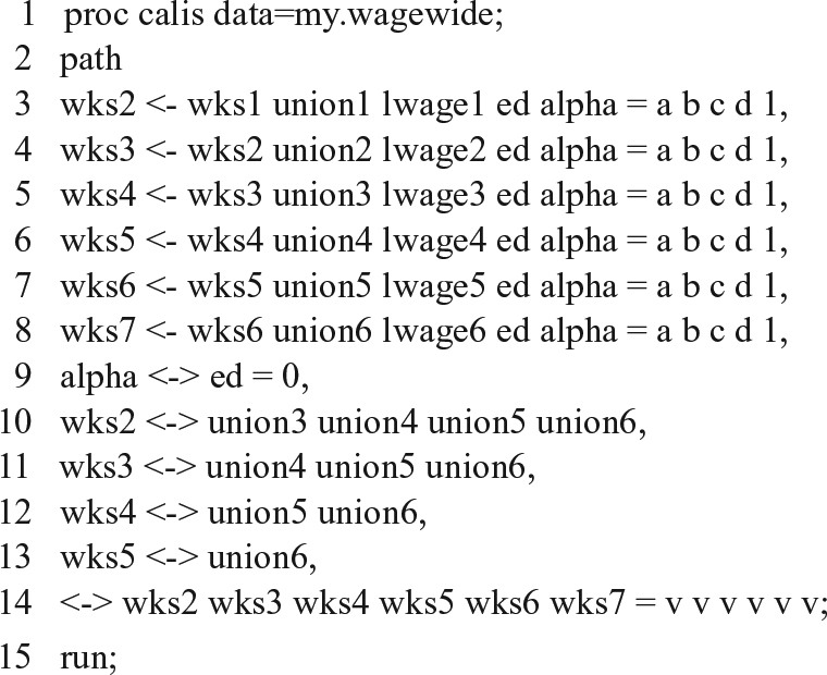
SAS program for estimating dynamic panel model with fixed effects.

The variable ALPHA refers to the “fixed effects” variable α _i that is common to all equations. When CALIS encounters a variable name like ALPHA that is not on the input data set, it presumes that the name refers to a latent variable. After the equals sign on each line, there is a list of coefficient names or values corresponding to the predictor variables in the equation. Because the coefficient names are the same for each equation, the corresponding coefficients are also constrained to be the same. The coefficient of ALPHA is constrained to have a value of 1.0 in each equation, consistent with Equation 1.

By default in PROC CALIS, latent exogenous variables like ALPHA are allowed to covary with all observed exogenous variables, including WKS1 and all the LWAGE and UNION variables. This is exactly what we want to achieve for ALPHA to truly behave as a set of fixed effects (Allison and Bollen 1997; Bollen and Brand 2010; Teachman et al. 2001). However, because ED does not vary over time, the correlation between ALPHA and ED is not identified, so it is constrained be 0 in Line 9. Lines 10 through 13 allow the error term ε in each equation to be correlated with future values of UNION. This is the key device that allows UNION to be a predetermined (sequentially exogenous) variable. ⁴

By default, CALIS allows the intercept to differ for each equation, which is equivalent to treating time as a set of dummy variables. It is easy to constrain the intercepts to be the same if desired. With a little more difficulty, one can impose constraints that correspond to a linear or quadratic effect of time.

Also by default, the error variances are allowed to differ across equations, which is not the case for most AB software. Line 14 constrains the error variances to be the same for each equation to produce results that can be directly compared with AB estimates. This line assigns names to the error variances for each variable. Because they are given the same name (v), the corresponding parameter estimates are constrained to be the same. In most applications, however, it is probably better to leave the variances unconstrained.

Figure 3 is a path diagram for the model. Here are a few key points to note about this diagram:

• There is no correlation between ALPHA and ED.

• All other observed exogenous variables are freely correlated with one another.

• All error terms are correlated with future values for UNION. This implicitly allows for the possibility that y affects future x, with no restrictions on that relationship.

Figure 3.

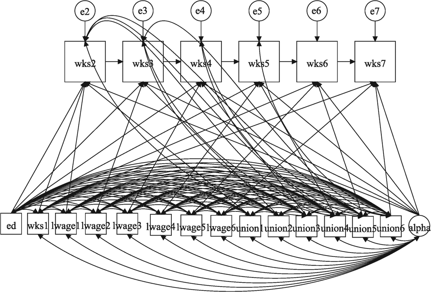
Path diagram for empirical example.

Table 1 displays the numerical results in the first four columns. Not surprisingly, there is a highly significant effect of WKS(t – 1) on WKS(t), although the magnitude of the effect is not large. There is also a significant negative effect (at the .05 level) of UNION(t – 1) on WKS(t) and a not quite significant negative effect of ED on WKS(t). By constraint, these coefficient estimates are the same for all six equations.

Table 1.

Alternative Estimates for Dynamic Model with Fixed and Lagged Effects.

	Maximum Likelihood Structural Equation Modeling			Arellano-Bond
Predictor	Estimate	SE	z	Estimate	SE	z
wks(t – 1)	.188	.020	9.59	.163	.039	4.18
lwage(t – 1)	.588	.488	1.20	−1.276	.462	−2.76
union(t – 1)	−1.206	.522	−2.31	−1.175	.513	−2.29
ed	−.107	.056	−1.89

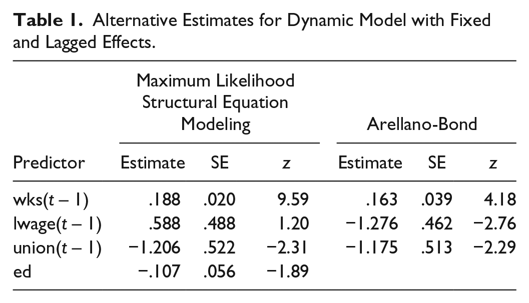
This is only a small portion of the output from PROC CALIS. The full output also contains estimates of the variances and covariances for all the exogenous variables, including ALPHA and the error terms for each equation. As with all SEM software, there is also a likelihood ratio chi-square statistic comparing the fitted model with a “saturated” or “just-identified” model that perfectly reproduces the covariance matrix for all the variables. For this example, it has a value of 138.48 with 76 degrees of freedom, yielding a p value less than .0001. The 76 degrees of freedom correspond to 76 over-identifying restrictions on the covariance matrix of the observed variables that are implied by the model.

Because this is a goodness-of-fit statistic, higher p values indicate a better fitting model. So by conventional significance standards, the model does not fit the data. However, the consensus in the SEM literature is that with large sample sizes, it may be hard to find any reasonably parsimonious model that yields a p value greater than .05. There are numerous alternative measures of fit that are relatively insensitive to sample size, and many of these are reported by PROC CALIS. For example, Bentler’s Comparative Fit Index is .995 while Bentler and Bonnet’s Non-Normed Index (also known as the Tucker-Lewis Index) is .987. ⁵ Values near 1.0 are desirable, so these measures suggest a very good fit to the data. One of the most popular measures of fit is the root mean square error of approximation (RMSEA). For this example, it has a value of .037. Anything less than .05 is considered to be a good fit.

For comparison, we also estimated the same model using the standard AB method, as implemented with the Stata command xtdpd. The last three columns of Table 1 display the results. Note that this method—because it is based on difference scores—cannot produce any estimates for the effect of ED, which does not change over time. ⁶ The lagged effects of UNION and WKS (on itself) are similar to the estimates produced by PROC CALIS. However, the coefficient for the lagged effect of LWAGE is dramatically different from the ML estimate. This naturally raises the question of which method performs better, in general.

Monte Carlo Study

To evaluate the performance of the ML-SEM method and compare it with the AB method, we generated observations from the following cross-lagged panel model:

$$\begin{array}{l}{y}_{i1}=c{\mathrm{\alpha }}_i+g{u}_{i1}\\ x_{i1}=c{\mathrm{\eta }}_i+g{v}_{i1}\\ y_{it}={\mathrm{\beta }}_1{x}_{it-1}+{\mathrm{\beta }}_2{y}_{it-1}+c{\mathrm{\alpha }}_i+g{u}_{it}\\ x_{it}={\mathrm{\beta }}_3{x}_{it-1}+{\mathrm{\beta }}_4{y}_{it-1}+c{\mathrm{\eta }}_i+g{v}_{it}\end{array}$$

for i = 1, . . . , N and t = 2, . . . T. The time-invariant “fixed effects,” α _i and η _i , were generated as bivariate standard normal variates with correlation ρ. The time-specific disturbances u_it and v_it were each standard normal and independent of all other exogenous variables. Parameters and data structures were varied as shown in Table 2.

Table 2.

Parameter Values for Monte Carlo Simulation.

N	50, 100, 400, 1,600
T	4, 5, 7, 10
ρ	0, .25, .50, .75, .90
β1	0, .25, .50, .75, 1.00
β2	0, .25, .50, .75, 1.00, 1.25
β4	–.25, 0, .25
g	.75, 1.00, 1.50, 2.00
c	.50, 1.00, 1.50, 2.00

Note: The numbers in bold are the values for the baseline model.

The numbers in bold are the values for the baseline model. Each parameter was varied in turn while keeping all others at their baseline values. For each condition, 1,000 samples were generated. There were a total of 30 different conditions.

For each sample, we estimated the parameters in the equation for y as the dependent variable using both ML-SEM and AB. We used Stata both to generate the data and estimate the models. The sem command ⁷ was used for ML-SEM, and the xtdpd command was used for AB. For the latter, we used the default one-step method with all available instruments. ⁸ Program code for the Monte Carlo simulations is available in an online appendix.

We will focus on the estimates for β₁, the cross-lagged effect of x on y, and β₂, the autoregressive effect of y on itself. For each of those parameters and for each condition, Appendix Table A.1 reports the mean and the standard deviation of the estimates for β₁ across the 1,000 samples as well as the “coverage”—the proportion of nominal 95 percent confidence intervals (calculated in each sample using the conventional normal approximation) that actually included the true values. If a method is performing well, the coverage should be close to .95.

Unlike AB, ML-SEM requires an iterative algorithm, and that algorithm sometimes fails to converge, especially with small samples and more extreme parameter values. Of the 30 conditions in the simulation, 12 had convergence failures for at least one of the 1,000 samples. For each condition, Appendix Table A.1 gives the number of convergence failures. Of those conditions that had convergence failures, the number of failures ranged from 1 to 23 (out of 1,000 samples). Thus, in the worst case, only about 2 percent of the samples suffered convergence failures.

Samples with convergence failures are likely to be more extreme or unusual than those without such failures, and the exclusion of those samples could give an unfair advantage to ML-SEM. To avoid that possibility, we also excluded the same nonconvergent samples from the AB estimation.

In Appendix Table A.1, both ML-SEM and AB estimators appear at first glance to produce approximately unbiased point estimates of β₁ (the cross-lagged effect of x on y) under all 30 conditions. However, the AB estimator actually shows a small downward bias under many conditions. Specifically, for AB, 11 of the thirty 95 percent Monte Carlo confidence intervals (not shown) do not include the true value because the upper confidence limit is less than the true value. For ML-SEM, on the other hand, every 95 percent Monte Carlo confidence interval includes the true value. Despite the downward bias in AB, the two estimators did about equally well for interval estimation. For both ML-SEM and AB, the median coverage over the 30 conditions was .949. ML-SEM coverage ranged from .934 to .957. For AB, the coverage ranged from .937 to .958.

For β₂ (the lagged effect of y on itself), AB does substantially worse than ML-SEM, as shown in Table A.2. Again, ML-SEM produces approximately unbiased estimates of β₂ under all conditions. Every 95 percent Monte Carlo confidence interval included the true value. On the other hand, AB estimates are persistently smaller than the true values, and only one of the 95 percent Monte Carlo confidence intervals included the true value. This downward bias is generally small, however, except for the smaller sample sizes of N = 50 and N = 100, where it’s quite apparent. Somewhat surprisingly, given earlier literature, the bias is small even when β₂ is at or close to 1.0.

The bias in AB for β₂ translates into slightly worse coverage for interval estimates. For ML-SEM, the median coverage over the 30 conditions was .951 with a range from .937 to .965. For AB, the median coverage was .941, ranging from .890 (for N = 50) to .961.

Next, we examine the relative efficiency of ML-SEM and AB. We calculate relative efficiency as the ratio of the estimated mean square error for ML-SEM to the estimated mean square error for AB. Mean square error is the sampling variance plus the square of the bias. Across 30 different conditions, the relative efficiency of AB compared with ML-SEM for estimating β₁ ranged from .83 (AB did 17 percent worse) to 1.12 (AB did 12 percent better), with a median of .96. So there was no clear winner for the cross-lagged effect. For β₂, however, the relative efficiency ranged from .34 (AB did 66 percent worse) to .87 (AB did 13 percent worse) with a median of .68. To put this in perspective, if the relative efficiency is .50, then using AB rather than ML would be equivalent to discarding half of the sample.

What affects relative efficiency? Although the relative efficiencies for all conditions are shown in the last column of Tables A.1 and A.2, we also present some of them here to highlight key results. Table 3 gives the relative efficiencies of the estimators for β₁ and β₂ as a function of the number of time points.

Table 3.

How Number of Time Points Affects Relative Efficiency of the Arellano-Bond Method.

	β1	β2
T = 4	1.040	.827
T = 5	.944	.708
T = 7	.939	.505
T = 10	.832	.337

For both β₁ and β₂, the relative efficiency of AB declines with the number of time points, although the decline is much more precipitous for β₂, the autoregressive coefficient. These declines are consistent with the literature suggesting that when there are many time points—and therefore many instruments—AB is vulnerable to overfitting.

Unfortunately, there is a potential problem with the results in Table 3. Because our data-generating model was not constrained to be stationary, the variances and covariances at later time points may have differed from those at earlier time points. So the declines in efficiency observed in Table 3 could reflect not the number of time points but rather changes over time in the pattern of variances and covariances. To avoid this possible confounding, we first produced approximate stationarity by generating data from 1,000 time points. Then, for the T = 4 condition, we used the data from the next four time points to estimate the model. The same strategy was used for T = 5, 7, and 10. Results in Table 4 show that the ML and AB estimators do about equally well for β₁ regardless of the number of time points. For β₂, however, the efficiency of AB is quite low at all time points and declines noticeably as the number of time points grows larger. In this case, the inferiority of AB stems both from downward bias in the coefficients and from larger standard errors.

Table 4.

Number of Time Points and Relative Efficiency under Approximate Stationarity.

	β1	β2
T = 4	.982	.562
T = 5	.989	.527
T = 7	1.038	.371
T = 10	1.029	.305

Previous work (Kiviet 2005) has suggested that the ratio of the fixed effects variance to the error variance may be an important factor in the efficiency of AB. Table 5 confirms this for β₂ but not for β₁. When the standard deviations of α and η are held constant at 1.0, increases in the standard deviations of ε and υ are associated with declines in the relative efficiency of AB for β₂ but not for β₁. The direction is reversed when the standard deviation of ε is held constant and the standard deviation of α is varied—higher standard deviations of α result in higher relative efficiency of AB for β₂.

Table 5.

How Relative Efficiency Depends on the Variance of ε and α.

	β1	β2
SD(ε) = .25	.924	.716
SD(ε) = 1.0	.944	.708
SD(ε) = 1.5	.974	.640
SD(ε) = 2.0	.964	.570
SD(α) = .5	.981	.629
SD(α) = 1.0	.944	.708
SD(α) = 1.5	.989	.814
SD(α) = 2.0	.974	.863

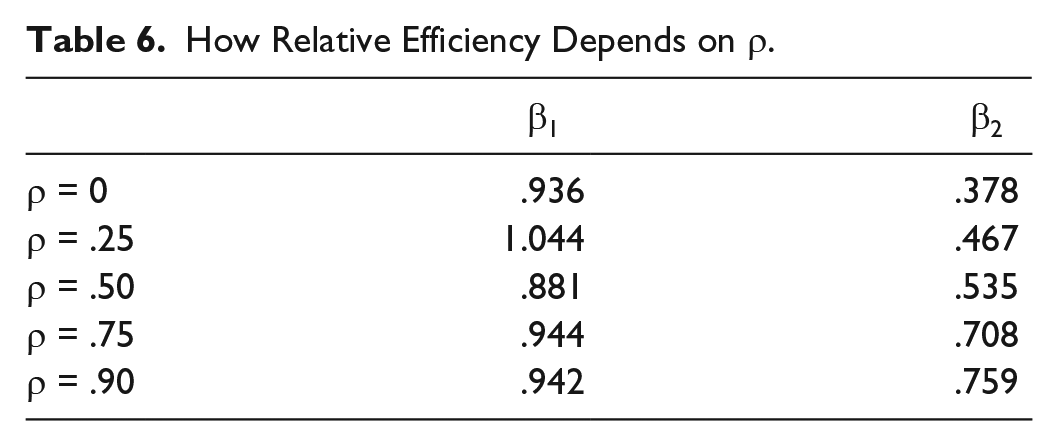
Table 6 shows how relative efficiency is affected by the value of ρ, the correlation between the two fixed effects, α and η. For β₁, there is no apparent trend. For β₂, however, the relative efficiency of AB increases substantially as the correlation goes from 0 to .90.

Table 6.

How Relative Efficiency Depends on ρ.

	β1	β2
ρ = 0	.936	.378
ρ = .25	1.044	.467
ρ = .50	.881	.535
ρ = .75	.944	.708
ρ = .90	.942	.759

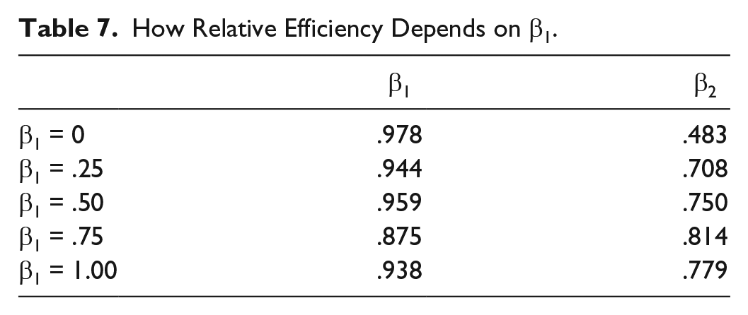
Finally, Table 7 shows how relative efficiency is affected by the magnitude of β₁, the cross-lagged coefficient. As in the last two tables, the relative efficiencies of AB estimates for β₁ are virtually unaffected. For β₂, relative efficiency increases substantially as β₁ gets larger.

Table 7.

How Relative Efficiency Depends on β₁.

	β1	β2
β1 = 0	.978	.483
β1 = .25	.944	.708
β1 = .50	.959	.750
β1 = .75	.875	.814
β1 = 1.00	.938	.779

There were three other factors that had no apparent effect on relative efficiency: the sign of β₄ (the cross-lagged effect of y on x), sample size, and the magnitude of β₂ (the autoregressive coefficient). The absence of a relationship with sample size and β₂ is somewhat surprising. We expected ML-SEM to do better in smaller samples, and we expected AB to perform more poorly when β₂ was close or equal to 1.0. In fact, AB did quite well when β₂ = 1, both in absolute terms and relative to ML-SEM.

Because ML-SEM is based on the assumption of multivariate normality, it has been suggested that it may do worse than AB when distributions are not normal. To check this out, for the baseline set of parameter values, all the random draws were made from a chi-square distribution with two degrees of freedom, a distribution that is highly skewed to the right. The last rows of Tables A.1 and A.2 show that both estimators did well under this condition, but ML-SEM did better. The relative efficiency of AB was .908 for β₁ and .619 for β₂.

Discussion and Conclusion

Panel data have a lot of potential for improving our ability to make causal inferences from non-experimental data. But appropriate methods are needed take advantage of such data. The linear dynamic panel model of econometrics protects against two major threats to valid causal inference: unmeasured confounders and reverse causation. The Arellano-Bond method can produce approximately unbiased estimates of the parameters of that model under a wide range of conditions. One of our goals was to show that cross-lagged panel models can be estimated within this econometric framework by estimating each side of the cross-lagged model separately. Compared with simultaneous estimation, this approach has the advantage producing estimates that are robust to misspecification of the lag structure or the functional form of the other side.

Unfortunately, the AB method is reputed to be problematic when the autoregressive parameter is near 1.0, and its efficiency has also been questioned. Maximum likelihood methods based on first differences have been offered as an alternative, but they rely on questionable assumptions about the initial conditions.

In this article, we have shown that the linear dynamic panel model with predetermined regressors is a special case of the well-known linear structural equation model. Instead of relying on difference scores to eliminate the fixed effects, maximum likelihood estimation of this model is accomplished by allowing the fixed effects to have unrestricted correlations with the time-varying predictors. The initial observations of the dependent variable are treated just like any other exogenous variables. Cross-lagged causation is accommodated by allowing the error term in each equation to correlate with future values of the time-dependent predictors. Many different statistical packages, both freeware and commercial, can implement the ML-SEM method.

Monte Carlo simulations showed that ML-SEM produced approximately unbiased estimates under all the conditions studied. Confidence interval coverage was also excellent. The AB estimator also did very well for the cross-lagged parameter, although with some downward bias. For the autoregressive parameter, however, the downward bias in AB was much more substantial, and its efficiency (relative to ML-SEM) was poor under most conditions. For this parameter, the efficiency of AB relative to ML-SEM also declined markedly as the number of time points increased.

So one key conclusion from the simulations is that if you are primarily interested in the cross-lagged coefficients, AB and ML-SEM have statistical properties that are about equally good. Nevertheless, there are still plenty of reasons why one might prefer ML-SEM. As detailed by Bollen and Brand (2010), the ML-SEM method can be extended in several ways. Although maximum likelihood is the default estimator for all SEM packages, most packages offer alternative methods, including the asymptotic distribution free method of Browne (1984). Many packages also have options for robust standard errors. Many of the constraints that are implied by the linear dynamic panel model can be easily relaxed in the SEM setting. We already showed how the error variances can be allowed to vary with time. One could also allow the coefficients to vary with time.

It’s even possible to allow the coefficient of α, the fixed effect, to vary with time instead of being constrained to 1 for every time point. This option is attractive because it removes one of the principal limitations of the classic fixed effects estimator: that it does not control for unmeasured time-invariant variables when their effects change over time. It is also possible to allow for individual-specific trends that are correlated with the time-varying predictors (Teachman 2014).

With regard to unbalanced samples and missing data more generally, most SEM packages have the option of handling missing data by FIML. Unlike AB, FIML can easily handle missing data on predictor variables. ⁹

Although we have not considered models with simultaneous reciprocal effects, such effects can certainly be built into SEM models if appropriate instruments are available. Finally, some SEM packages (like Mplus or the gsem command in Stata) can estimate similar models for categorical dependent variables.

Are there any downsides to ML-SEM? As noted earlier, ML-SEM is not suitable when T is large relative to N. This is easily seen from the fact that ML-SEM operates on the full covariance matrix for all the variables at all points in time. For example, if the predictors in the model consist of nine time-varying variables and T = 11, then the covariance matrix will be 101 × 101. And unless N > 101, that matrix will not have full rank, causing the maximization algorithm to break down. As noted earlier, ML-SEM will sometimes fail to converge. And even if it converges, computation time can be considerably greater than for AB, especially when using FIML to handle missing data.

As can be seen from Figure 2 and Appendix B, program code for ML-SEM can be more complex than for the AB method. Not only are ML-SEM programs typically longer, but it can also be challenging for the analyst to figure out exactly how to specify the model so that the correct covariances are either set to 0 or left unconstrained. This challenge is exacerbated by the fact that different packages have different defaults for the covariances and different ways of overriding those defaults.

Of course, this is just a programming issue, and it would certainly be feasible to write a Stata command, a SAS macro, or an R function that would automatically set up the correct model with minimal input from the user. As noted earlier, we have already developed a Stata command called xtdpdml that does exactly that (Williams, Allison, and Moral-Benito 2016). This command radically reduces the programming needed for ML-SEM and is actually simpler to use than the built-in Stata commands for AB estimation (xtabond, xtdpd, or xtdpdsys).