How to Deal With Reverse Causality Using Panel Data? Recommendations for Researchers Based on a Simulation Study

Abstract

Does X affect Y? Answering this question is particularly difficult if reverse causality is looming. Many social scientists turn to panel data to address such questions of causal ordering. Yet even in longitudinal analyses, reverse causality threatens causal inference based on conventional panel models. Whereas the methodological literature has suggested various alternative solutions, these approaches face many criticisms, chief among them to be sensitive to the correct specification of temporal lags. Applied researchers are thus left with little guidance. Seeking to provide such guidance, we compare how different panel models perform under a range of different conditions. Our Monte Carlo simulations reveal that unlike conventional panel models, a cross-lagged panel model with fixed effects not only offers protection against bias arising from reverse causality under a wide range of conditions but also helps to circumvent the problem of misspecified temporal lags.

Introduction

Many studies in the social sciences try to answer questions about causal relationships such as: Does bad pay cause occupations to feminize (England, Allison, and Wu 2007)? Is the risk of divorce increased by limited financial resources (Killewald 2016)? What is the effect of social contacts on labor market success (Mouw 2006)? Most methodologists consider controlled randomized experiments as the “gold” standard for causal inference (Imbens and Rubin 2015; Rosenbaum 2017). Useful as they are, however, experiments are hardly a silver bullet for social science research. Many interesting variables related to human behavior and its consequences—such as working conditions, family life, or social contacts—are difficult to manipulate, with ethical, political, and practical restrictions forcing researchers to deviate from the experimental ideal (Shadish, Cook, and Campbell 2002). More often than not, social scientists therefore have to rely on observational data for causal inference (e.g., Morgan and Winship 2015).

Panel data have become particularly prominent for causal inference based on observational data (Bell and Jones 2015; Brüderl and Ludwig 2015; Imai and Kim 2019). A key reason for the popularity of panel models is that they allow to exploit change within units over time (e.g., individual change) to eliminate unobserved time-invariant heterogeneity, which considerably reduces the risk of confounding (Allison 2009; Halaby 2004; Wooldridge 2010). Moreover, researchers frequently turn to panel data since they expect them to determine causal order (Vaisey and Miles 2017). Reconsidering the abovementioned research questions, one might ask: Does feminization of occupations reduce pay? Do spouses adjust their work behavior in anticipation of marital problems? Do successful people associate with one another? As these examples illustrate, the causal arrow often might run in both directions or even only in the other direction. Establishing causal order by accounting for reverse causality therefore is a key challenge in many social scientific areas of research. ¹

In stark contrast to the well-known issue of unobserved heterogeneity, however, it is much less clear for researchers how to deal with reverse causality. Even with panel data, it is far from trivial to identify the causal effect of X on Y if reverse causality is present. Having long recognized this problem, the econometric and statistical literature has developed various models to disentangle the dynamic interplay of X and Y with observational data. This includes first-difference (FD) models with lagged independent variables (Allison 2009), dynamic panel models relying on instrumental variables (Arellano and Bond 1991), cross-lagged structural equation models (Finkel 1995), and, more recently, cross-lagged panel models with fixed effects (FE; Allison, Williams, and Moral-Benito 2017). Yet the number of suggestions seems to equal the number of critics (e.g., Bellemare, Pepinsky and Masaki 2017; Reed 2015), some of which even conclude that none of the abovementioned models solves the problem of reverse causality under general conditions (Brüderl and Ludwig 2015). ²

Further complicating the matter for applied researchers, Vaisey and Miles (2017) recently showed that panel models are sensitive to the correct specification of temporal lags. Specifically, they demonstrated that lagged first-difference (LFD) models provide highly misleading estimates if the effect of X on Y is not fully lagged as captured by the observed data. However, it is an open question whether this problem also applies to other panel models. Even more importantly, applied researchers currently find little guidance other than the warning not to “rely on the ordering of the data to establish causal priority unless the lags between panels match the real-world causal lags in the processes under study” (Vaisey and Miles 2017:64). While this advice is well justified, it does not address the question what researchers can do if they face reverse causality and/or are uncertain about the precise temporal nature of the “real-world causal lags.”

In sum, the absence of clear modeling standards leaves researchers uncertain how to deal with reverse causality in panel models and what to do if the timing of causal effects is unknown. Aiming to provide such guidance, we first give a short overview of existing approaches by discussing respective models and their key assumptions regarding reverse causality. We then simulate panel data in order to assess how different panel models perform under varying conditions. Specifically, we vary the degree of time-invariant unobserved heterogeneity, the presence of reverse causality, and the temporal lags of the causal effect of X on Y. Based on the results, we identify different scenarios for which certain panel models are adequate. We conclude with recommendations for researchers on how to deal with reverse causality in practice.

Panel Models in Face of Reverse Causality

In the following three subsections, we review different panel models, focusing on their exogeneity assumptions. These assumptions are not only crucial for understanding why reverse causality threatens conclusions derived from models that assume strict exogeneity but also offer a potential solution to the problem by relaxing this assumption. ³ For the sake of simplicity, we assume a balanced panel with n = 1,…, N, units of analysis, t = 1,…, T, panel waves, and NT observations, but the core assumptions about reverse causality also extend to unbalanced panels. We further focus on identifying the effect of X on Y, thus considering reverse causality—the effect of Y on X—as a nuisance that threatens causal inference rather than a substantive phenomenon one is interested in. ⁴

Panel Models Assuming Strict Exogeneity

Consider we want to estimate the effect of a set of variables X on an outcome variable Y using panel data. A good starting point for introducing models for microlevel panels with large N and small T is the pooled OLS (POLS) model,

$y_{it}={\beta }_1{x}_{it}+{\beta }_2{Z}_i+{\epsilon }_{it},$

which maps the outcome variable $y_{it}$ as an additive linear function of the time-varying variables $x_{it}$ , a vector of time-invariant covariates Z_i , and an error term ${\epsilon }_{it}$ that is assumed to be independent and identically distributed. Unbiased and consistent estimation is achieved if the error term is contemporaneously exogenous, that is, if it is not correlated with contemporaneous values of the independent variables:

$\text{Ε}\left({\epsilon }_{it}|x_{it},Z_i\right)=0.$

While generally allowing for the possibility of reverse causality, within POLS, causal inference for the effect of a variable X on Y is valid only if the model adequately captures all variables that simultaneously affect X and Y. Unfortunately, this strong assumption is rarely met in empirical applications, as many confounders either might not have been measured adequately or were not observed in the first place (see Brüderl and Ludwig 2015; Halaby 2004). POLS estimates therefore face an inherent risk of bias due to unmeasured unit-specific confounders that violate the key assumption of contemporaneous exogeneity.

A next natural step is to decompose the error term into a unit-specific part ${\alpha }_i$ and an idiosyncratic part ${\epsilon }_{it}$ in order to estimate a model that simultaneously covers both sources of error. There are two major approaches of how to treat the unit-specific error term ${\alpha }_i$ . The first approach is the FE model, which allows the unit-specific error term ${\alpha }_i$ to be correlated with the independent variables and removes between-unit heterogeneity by estimating unit-specific constants or, equivalently, by subtracting unit-specific means from X and Y (here and in the following, see Allison 2009; Brüderl and Ludwig 2015; Wooldridge 2010). In contrast to POLS, uncontrolled influences of unit-specific confounders Z_i , also called time-invariant unobserved heterogeneity, do not bias FE estimates because all time-invariant unobserved heterogeneity is fully captured by the unit-specific error term ${\alpha }_i$ . For the FE model, the equation hence does not contain time-invariant variables and reduces to

$y_{it}=\beta x_{it}+{\alpha }_i+{\epsilon }_{it}.$

The second approach is the random effects (RE) model. The RE model also includes a unit-specific error term ${\alpha }_i$ , but unlike in the FE model, this unit-specific error term is assumed to be uncorrelated with the independent variables, being treated as a random variable following a certain probability distribution, usually the standard normal distribution with mean zero and constant variance ${\sigma }_{\alpha }^2:{\alpha }_i\sim N(0;{\sigma }_{\alpha }^2)$ . In contrast to the FE model, the RE model therefore can provide estimates for time-invariant variables, but this comes at the cost of requiring an additional exogeneity assumption about time-invariant unobserved heterogeneity:

$\text{Ε}({\alpha }_i|x_{it},Z_i)=0.$

Despite these differences of the FE and the RE models in handling unobserved heterogeneity, they share the core assumption of strict exogeneity:

$\text{Ε}\left({\epsilon }_{is}|x_{it},{\alpha }_i\right)=0\text{ for all}s,t=1,\dots ,T.$

The key point is that this assumption is necessarily violated in case of reverse causality. Strict exogeneity forbids current values of ${\epsilon }_{is}$ to be correlated with past, present, and future values of $x_{it}$ . However, if $y_{it}$ affects $x_{it+1}$ , that is, if reverse causality is present, ${\epsilon }_{it}$ is necessarily correlated with $x_{it+1}$ . By violating one of the core assumptions of both RE and FE models, the presence of reverse causality thus introduces bias to estimates from both models. As Bellemare, Pepinsky, and Masaki (2017) show, many scholars hope to overcome this problem by lagging the independent variables in their panel data models (also see Reed 2015):

$y_{it}=\beta x_{it-1}+{\alpha }_i+{\epsilon }_{it}.$

The idea behind this approach is that while ${\epsilon }_{it}$ is correlated with $x_{it+1}$ in case of reverse causality, ${\epsilon }_{it-1}$ may be not. Yet as Reed (2015) demonstrates both analytically and with simulations, reverse causality also biases point estimates and statistical inference in these models. Bellemare et al. (2017) explain why endogeneity problems also occur with this approach: While lagging the independent variable helps to get rid of the strong and untestable strict exogeneity assumption, it introduces the similarly strong and untestable assumption that unobserved variables are serially uncorrelated. Identification requirements in models with lagged independent variables thus are usually similarly strong as those in models with contemporaneous values of X. Therefore, simply lagging X in RE or in FE models rarely solves the endogeneity problem posed by unobserved variables (see Bellemare et al. 2017:960).

Panel Models Relaxing the Strict Exogeneity Assumption

The key takeaway message from the previous section is that relaxing the assumption of strict exogeneity is needed for dealing with reverse causality. One such approach is offered by a close relative of the FE model, the FD model. Instead of controlling for time-invariant unobserved heterogeneity by demeaning the data, the FD model eliminates ${\alpha }_i$ by means of subtraction of first order (see Lee 2016, for a generalization of the differencing method). Suppose separate equations for two time points:

$\begin{array}{c}{y}_{it}={\beta }_1{x}_{it}+{\beta }_2{Z}_i+{\alpha }_i+{\epsilon }_{it}\\ y_{it-1}={\beta }_1{x}_{it-1}+{\beta }_2{Z}_i+{\alpha }_i+{\epsilon }_{it-1}.\end{array}$

Taking the difference of these equations removes both the unit-specific error ${\alpha }_i$ and all time-invariant regressors Z_i :

$\Delta y_{it}=\beta \Delta x_{it}+\Delta {\epsilon }_{it}.$

Since the unit-specific error term ${\alpha }_i$ disappears from the equation after calculating the first difference, the FD model requires no exogeneity assumption about ${\alpha }_i$ . Furthermore, like the FE model, the FD model assumes strict exogeneity for unbiased estimation of the effects of independent variables $x_{it}$ (Wooldridge 2010:316). However, as Cameron and Trivedi (2009:264) note, the FD model rests on a weaker version of the exogeneity assumption than the FE model, since the FD model uses only values from the previous wave for differencing, whereas the FE model uses all past and future values for calculating within deviations from person-specific means (Halaby 2004:534). This fact can be exploited in the FD framework to deal with situations in which Y affects X.

In particular, a LFD model has been suggested in order to tackle reverse causality (Allison 2009; for empirical applications, see England et al. 2007; Leszczensky 2013; Levanon, England and Allison 2009; Martin, Van Gunten, and Zablocki 2012). The model is specified as follows:

$y_{it}-y_{it-1}=\beta (x_{it-1}-x_{it-2})+({\epsilon }_{it}-{\epsilon }_{it-1}).$

Compared to FE or RE models, the LFD model promises to offer protection not only against bias arising from unobserved time-invariant heterogeneity but also from reverse causality. The former is achieved by eliminating the unit-specific error term ${\alpha }_i$ by taking first differences, the latter by allowing for a causal feedback process of X on Y by permitting a correlation of $x_{it}$ with future values of ${\epsilon }_{it}$ .

Unfortunately, though, as Vaisey and Miles (2017) recently showed, estimates from the LFD model suffer from severe bias if the model does not adequately depict the true timing of causal effects. This is because the LFD model rests on the crucial assumption that the change of Y between two points in time is indeed a function of the specified difference of X between two preceding points in time. Yet as Vaisey and Miles (2017) demonstrate in simulations with three panel waves, if the true causal effect of X on Y is contemporaneous rather than lagged, the LFD model substantially underestimates the true effect size and provides estimates that go in the opposite direction. Whether or not the application of the LFD model is appropriate thus crucially depends on whether or not the lags in the panel data match the real-world causal lags in the process under study. This risk of specification error highlights the need for precise theorizing regarding the actual lag structure of the causal process under investigation. The LFD model accordingly is hardly a panacea for dealing with reverse causality; in fact, it can do more harm than good if it is applied without precise theoretical knowledge about the underlying data generating process or if the temporal lags in the available data simply do not match the actual causal process.

Dynamic Panel Models Allowing for Both Strict and Sequential Exogeneity

In addition to the LFD model, dynamic panel models have been suggested to address the endogeneity problem caused by reverse causality. Dynamic panel models try to map the interplay between X and Y over time by including lagged values of the dependent variable on the right-hand side of the equation:

$y_{it}={\beta }_1{y}_{it-1}+{\beta }_2{x}_{it}+{\alpha }_i+{\epsilon }_{it}.$

However, as Nickell (1981) has shown, including a lagged-dependent variable (LDV) in FE or RE models necessarily induces a correlation of the idiosyncratic error ${\epsilon }_{is}$ and the LDV, thus violating the strict exogeneity assumption and resulting in biased estimates, as shown above. This so-called dynamic panel or Nickell bias is particularly large for microlevel panels with large N and small T but can remain quite substantial for larger T (e.g., T >10). Furthermore, if the LDV is correlated with X, the estimates for these independent variables are also biased.

One prominent econometric model to resolve this issue has been suggested by Anderson and Hsiao (1981, 1982) and extended and popularized by Arellano and Bond (1991). Since the LDV from the first lag is correlated with ${\epsilon }_{is}$ , these dynamic panel estimators take first differences to remove time-invariant unobserved heterogeneity:

$\Delta y_{it}={\beta }_1\Delta y_{it-1}+{\beta }_2\Delta x_{it}+\Delta {\epsilon }_{it}.$

Then $y_{it-2}$ , the LDV from second-order lags of Y is used as an instrumental variable (IV) for $\Delta y_{it-1}$ (Anderson and Hsiao 1981, 1982). Whereas this early IV estimator only uses a small proportion of all available instruments, namely one instrument for each panel wave, the nowadays commonly used generalized method of moments (GMM; see Hansen 1982) increases efficiency by estimating a set of equations with varying number of instruments depending on the number of available previous panel waves. Arellano and Bond (1991) recommend to use all preceding levels of the LDV ( $y_{it-2}, y_{it-3},\dots$ ) as instruments (standard or difference GMM; see also Holtz-Eakin, Newey, and Rosen 1988), while extensions highlighted the value of using FDs of the LDV ( $\Delta y_{it-2}, \Delta y_{it-3},\dots$ ) or combinations of both sets of variables as instruments (system GMM; Arellano and Bover 1995; Blundell and Bond 1998).

The important point is that both types of GMM estimators allow distinguishing between strictly exogenous variables on the one hand and sequentially exogenous, so-called predetermined, variables on the other. As in case of FE or RE models, strictly exogenous variables are not allowed to be correlated with past, present, and future values of the error term. By contrast, predetermined variables are assumed to be sequentially exogenous. Like strict exogeneity, sequential exogeneity forbids the current idiosyncratic error ${\epsilon }_{is}$ to be correlated with previous and current values of $x_{it}$ . Unlike strict exogeneity, however, it allows for current values of ${\epsilon }_{is}$ to be correlated with future values of $x_{it}$ :

$\text{Ε}\left({\epsilon }_{is}|x_{it}\right)=0 \hspace{1em}\text{for} t\le s.$

Independent variables that are assumed to be predetermined are treated in a similar way as Y is in the Arellano-Bond (AB) model, that is, they are instrumented using lagged values of the same independent variable. Compared to RE and FE models, AB-type panel estimators thus weaken the exogeneity assumption for a subset of regressors, thereby providing consistent estimates even if reverse causality is present. ⁵

In principle, the AB estimator and related dynamic panel models offer a powerful toolbox to tackle endogeneity problems caused by both reverse causality and unobserved heterogeneity. However, despite its wide application in econometrics, the approach is known to suffer from downward bias in face of a large number of moment conditions (Hsiao 2007:90) and weak instruments problems (Bun and Windmeijer 2010), both of which can undermine causal inference. In addition, AB estimators show poor finite-sample performance (Newey and Windmeijer 2009) and require a large number of sampled units (Moral-Benito, Allison, and Williams 2018).

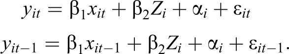
The cross-lagged panel model with FE addresses some of these concerns. It is based on work by Moral-Benito (2013) who showed that a dynamic panel model with lagged independent variables and FE can be estimated by maximum likelihood without taking FDs and without any assumptions about initial observations of X and Y. Allison, Williams, and Moral-Benito (2017) further showed that the maximum likelihood (ML) method suggested by Moral-Benito (2013) can be implemented in a structural equation modeling (SEM) framework, hence calling it the ML-SEM method (also see Bollen and Brand 2010 for a general structural equations approach to panel models). ⁶ Consider the following equation:

$y_{it}={\beta }_1{y}_{it-1}+{\beta }_2{x}_{it-1}+{\beta }_3{Z}_i+{\alpha }_i+{\epsilon }_{it},$

which includes lagged values of the dependent variable $y_{it-1}$ and a random error term ${\epsilon }_{it}$ . ${\alpha }_i$ represents the combined time-invariant effects of all time-invariant unobserved variables, thus being a unit-specific FE. ML-SEM, however, does not treat ${\alpha }_i$ as a fixed parameter but as a latent variable that is allowed to correlate with $x_{it}$ and $y_{it}$ at all points in time. ML-SEM thus provides FE estimates for time-varying covariates (see also Allison 2009; Bollen and Brand 2010), while initial values of Y and X are treated as strictly exogenous. Similar to the RE model, if unit-specific regressors Z_i are included, as in the above equation, it is further necessary for identification of the effects of Z_i to assume that they are uncorrelated with ${\alpha }_i$ .

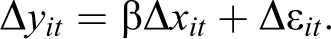
The equation above can then be reproduced within the SEM framework. Following Allison et al. (2017), Figure 1 illustrates the model for T = 4. For the ease of model presentation, covariates Z_i are not displayed. Like the LFD model and AB-type estimators, the ML-SEM method allows for reverse causality by assuming sequential exogeneity for $x_{it}$ . As explained before, residuals ${\epsilon }_{it}$ are allowed to correlate with all future values of such predetermined explanatory variables. In Figure 1, this is illustrated by the bidirectional arrow between x ₃ and ${\epsilon }_2$ , which allows a reverse causal effect from Y on X. The other correlations between the predetermined variable X and the error term for Y at any prior time point are omitted from the graph for ease of illustration. At the same time, it is possible to assume strict exogeneity for a subset of regressors that are expected to be uncorrelated with previous values of Y and to estimate the effects of time-invariant variables, not just control them as in the FE and FD model. We omit both types of predictors, as they do not affect the considerations regarding reverse causality. Importantly, as illustrated by the absence of arrows between ${\epsilon }_{2 },{\epsilon }_3,\text{ and }{\epsilon }_4$ in Figure 1, ML-SEM rests on the assumption of no serial correlation of errors.

Figure 1.

Path diagram for four-period ML-SEM. Source: Allison et al. (2017:6).

In Monte Carlo simulations, Moral-Benito (2013), Allison et al. (2017), and Moral-Benito et al. (2018) show that applying the ML-SEM method to the cross-lagged panel model with FE seems to keep the promise of offering protection against both time-invariant unobserved heterogeneity and reverse causality. Comparing ML-SEM and AB estimators, all three simulation studies highlight advantages of ML-SEM regarding unbiasedness efficiency, and finite sample performance.

However, these earlier simulations do not consider the problem raised by Vaisey and Miles (2017), that is, that inference based on FD models is prone to bias due to misspecification of temporal lags. ⁷ Hence, like for RE, FE, and AB models, it remains open whether the ML-SEM method for cross-lagged panel models with FE is sensitive to the correct specification of temporal lags.

Summary

Let us briefly summarize our discussion of different panel models and their exogeneity assumptions, which are crucial for addressing reverse causality. As is well known, the POLS and the RE model will provide biased estimates if reverse causality and/or time-invariant unobserved heterogeneity are present because both of them introduce endogeneity and therefore violate the key exogeneity assumptions. While the FE and the FD model provide protection against endogeneity arising from unobserved heterogeneity, they also yield biased estimates in case of reverse causality because reverse causality violates the assumption of strict exogeneity. In contrast, the LFD model accounts for both time-invariant unobserved heterogeneity and reverse causality by relaxing the strict exogeneity assumption and only requiring sequential exogeneity. As shown by Vaisey and Miles (2017), however, the LFD model only provides unbiased estimates if the effect of X on Y is indeed fully lagged, thus being prone to specification error. Finally, the AB and ML-SEM models also promise to perform well in case of time-invariant unobserved heterogeneity and/or reverse causality, the latter of which is achieved by assuming sequential rather than strict exogeneity. However, it is an open question whether these models are also sensitive to the specification of temporal lags.

Simulation Study

In order to assess how different panel models perform under different conditions regarding reverse causality, we simulate panel data varying the degree of unobserved heterogeneity, the extent of reverse causality, and the temporal nature of the causal effect of X on Y.

Consider two random variables, Y and X, which might have a reciprocal causal relationship, as well as a vector of time-invariant variables Z_i that have time-invariant effects on both Y and X. To determine the starting values $y_{i0}$ and $x_{i0}$ , we drew correlated random variables (r = 0.5) and added a standard normally distributed independent error term ${\epsilon }_{it}$ to Y and ${\mu }_{it}$ to X. Then, the data generating process was set into motion by the following two equations:

$y_{it}={\beta }_1{y}_{it-1}+(1-\lambda ){\beta }_2{x}_{it}+\lambda {\beta }_3{x}_{it-1}+{\beta }_4{Z}_i+{\epsilon }_{it}\hspace{1em}\text{with}\hspace{1em}{\epsilon }_{it}\sim N(0;1),$

$x_{it}={\beta }_5{y}_{it-1}+{\beta }_6{Z}_i+{\mu }_{it}\hspace{1em}\text{with}\hspace{1em}{\mu }_{it}\sim N(0;1).$

The parameter ${\beta }_1$ influences the degree of autocorrelation of the outcome variable Y in the data. ⁸ This effect of $y_{it-1}$ on $y_{it}$ was set to 0.2, 0.5, or 0.8 in the simulation. Because the extent of autocorrelation did not substantially affect the results, we condense our findings by only reporting results for ${\beta }_1=0.5$ in the following (but see Section A of the Online Supplementary for the results if ${\beta }_1=0.2$ or ${\beta }_1=0.8$ ).

The parameters ${\beta }_2$ and ${\beta }_3$ map the causal effects of interest and are set to 1. Following Vaisey and Miles (2017), we introduced the parameter $\lambda$ to switch between contemporaneous and lagged effects of X on Y. For $\lambda =0$ , the effect is purely contemporaneous; for $\lambda =1$ , purely lagged; and for $\lambda =0.5$ , there is both a contemporaneous and a lagged effect, with an equal strength of 0.5. ⁹

Reverse causality is captured by the parameter ${\beta }_5$ , which is set to either 0 or 0.5. Finally, ${\beta }_4$ and ${\beta }_6$ give the time-invariant effects of time-invariant unit-specific variables on X and Y, thus representing unobserved heterogeneity. Time-invariant unobserved heterogeneity also is either absent (0) or present (0.5). ¹⁰

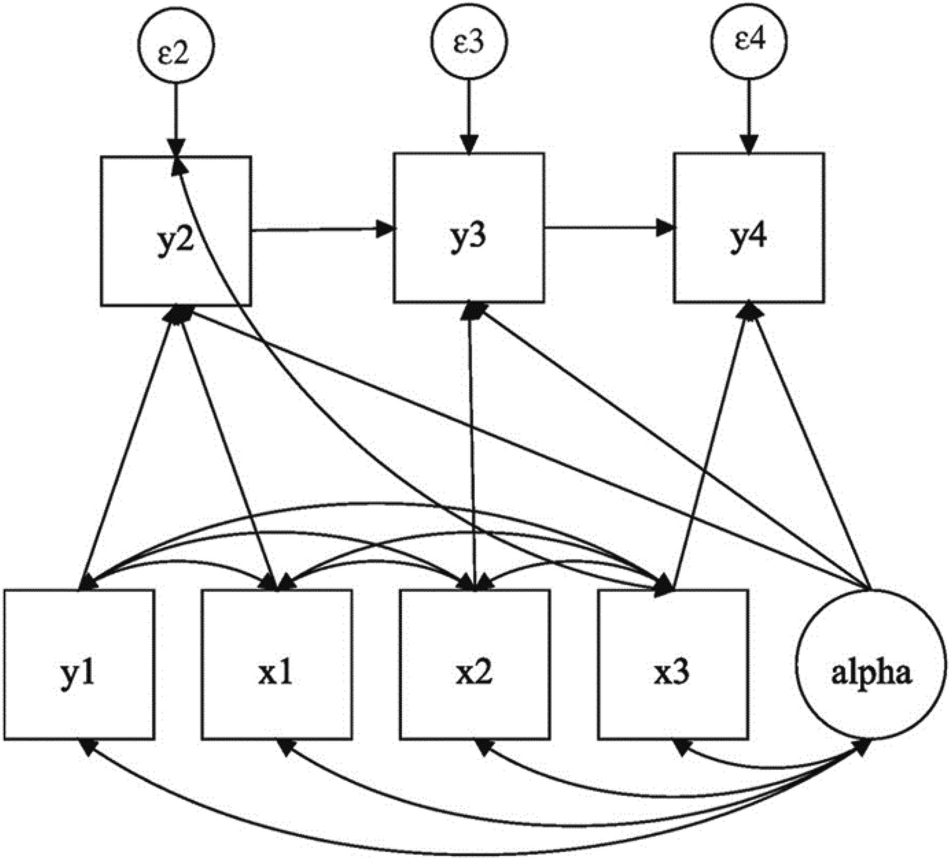
Table 1 summarizes the different parameters of the simulation and their possible values. In total, our simulation covers 3 × 3 × 2 × 2 = 36 scenarios. For each scenario, we simulated 500 data sets with N = 500 observations and T = 5 panel waves. ¹¹

Table 1.

Components of the Simulation and Parameter Values.

Parameter(s)	Concept	Values
${\beta }_1$	Autocorrelation	0.2; 0.5; 0.8
${\beta }_2/{\beta }_3$	Contemporaneous/lagged effect of X	1
$\lambda$	Contemporaneous versus lagged world	0; 0.5; 1
${\beta }_4/{\beta }_6$	Unobserved heterogeneity: Y/X	0; 0.5
${\beta }_5$	Reverse causality	0; 0.5

Based on these simulated data, we estimated the different panel models discussed above in order to assess their performance. To explore how the different models respond to the problem of wrong temporal lags, we used three different specifications for each model: one including only the contemporaneous effect of X, one including only the lagged effect of X, and one including both the contemporaneous and the lagged effect of X. The model that includes both a contemporaneous and a lagged effect is justified on two grounds. On the one hand, both contemporaneous and lagged values of X might affect Y; for example, marital problems can be caused both by past and by current financial problems. On the other hand, such a model corresponds to a situation in which substantive knowledge and theory are not precise enough to determine the correct temporal lag for the effect of X on Y. A model with both a contemporaneous and a lagged effect allows researchers to address this uncertainty by estimating both effects (for an approach to handle atheoretical lags, see also Cranmer, Rice, and Siverson 2017).

We estimated all models using Stata version 14.1. For the AB-estimators, we used the user-written command xtabond2 (Roodman 2012), which is more flexible than the standard Stata command. We rely on the approach advocated by Arellano and Bond (1991) taking FDs in a first step to remove unobserved heterogeneity and then using second- and higher order lags of the dependent variables as instruments in a standard GMM framework to deal with reverse causality. ¹² For the ML-SEM method, we used the user-written command xtdpdml, which serves as a shortcut for Stata’s sem command (Williams, Allison, and Moral-Benito 2018). In the ML-SEM, coefficients for the effects of X on Y, and vice versa, are constrained to be equal across all points in time. Our Stata code is publicly and permanently available at the Harvard Dataverse (Leszczensky and Wolbring 2019).

Results

We present results obtained from three different specifications of the six models discussed in Panel Models in Face of Reverse Causality section: the POLS model, the RE model, the FE model, the FD model, the AB estimator, and the cross-lagged model with fixed effects (ML-SEM). Following Vaisey and Miles (2017), we distinguish between three worlds that differ with respect to the timing of causal effects. In the contemporaneous world, x_t has an effect on y_t . In the lagged world, $x_{t-1}$ has an effect on y_t . Finally, in the mixed world, both x_t and $x_{t-1}$ affect y_t to a similar extent. We use the term “scenario” to further distinguish whether time-invariant unobserved heterogeneity and/or reverse causality affected the data generating process within these three worlds. This leaves us with four scenarios for each of the three worlds.

Contemporaneous World

We start by considering a world in which Y is only affected by the contemporaneous value of X, that is, in which $\lambda =0$ and, accordingly, the effect of $x_{it}$ is 1 and the effect of $x_{it-1}$ is 0. As noted above, such a world may be at odds with a causal inference perspective because cause and effect cannot occur at exactly the same point in time. Examining the performance of panel models in such a world is still informative, however, since in many empirical applications, the exact timing of a causal effect is unknown. For example, if both X and Y are repeatedly measured with panel gaps of one year, causal lags that are much shorter than the one-year gap between the points of observation might be more accurately captured by the contemporary effect of X on Y than by the lagged one.

Figure 2 shows how the different panel models perform in four different scenarios. The tabulated results of all models in Figure 2 are found in Section B in the Online Supplementary, as are all other models on which the following figures are based. The two horizontal lines in Figure 2 represent the true causal effects of $x_{it}$ (equal to 1) and $x_{it-1}$ (equal to 0). For all six models, we estimated one specification that only includes the contemporaneous effect of X on Y (depicted by a square), one that only includes the lagged effect of X on Y (depicted by a circle), and one that includes both effects (depicted by a triangle). The point estimates and 95 percent confidence intervals are averaged over the 500 runs of the simulation.

Figure 2.

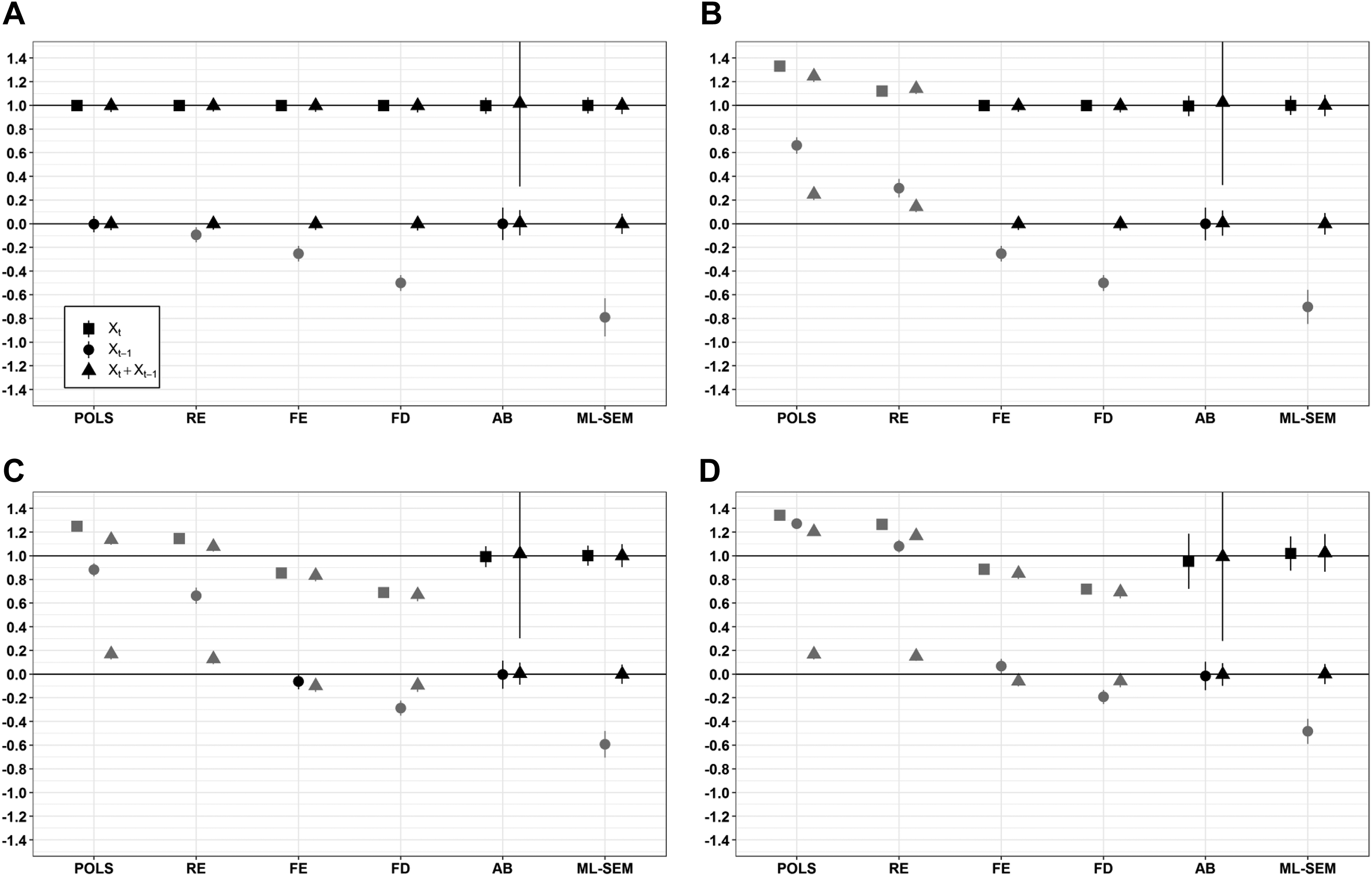
Simulation results for the contemporaneous world (n = 500, t = 5, 500 iterations; 95% confidence intervals). Unbiased estimates are colored in black, biased estimates in gray. The solid horizontal lines represent the true estimates.

Panel A in Figure 2 depicts the simplest possible scenario in which neither time-invariant unobserved heterogeneity nor reverse causality contributed to the data generating process. Although empirical applications rarely face the luxury of such an idealized scenario, it serves as a useful benchmark for comparison.

Starting with the models that only include the contemporaneous effect of X on Y (squares in Figure 2), from POLS to ML-SEM, all of them correctly identify the true effect of x_t . This is hardly surprising, of course, since the assumption of strict exogeneity as well as the weaker assumptions of contemporaneous and sequential exogeneity hold if neither time-invariant unobserved heterogeneity nor reverse causality are present.

Turning to the models that include only the lagged effect of X on Y (circles in Figure 2); however, most models fail to identify the lagged nil effect. The coefficient of the FD model (−0.5) replicates the finding by Vaisey and Miles (2017), that is, a LFD model produces biased estimates in the opposite direction of the true effect if the specification does not accurately map the actual causal process. Extending their finding, Figure 2 indicates that this problem of misspecified lags similarly applies to the RE, the FE, and the ML-SEM model, all of which yield significant negative coefficients even though no lagged effect contributed to the data generating process. In fact, only the POLS and the AB model correctly identify the lagged nil effect.

Finally, if both the contemporaneous and the lagged effect of X on Y are included in the estimation equation, all models correctly identify both effects (triangles in Figure 2). This finding suggests that it may be a promising approach to include both contemporaneous and lagged effects for addressing the problem of misspecified temporal lags. The question, however, is whether this approach also works in the other scenarios and worlds.

In the next scenario, we therefore added time-invariant unobserved heterogeneity to the data generating process. The results in panel B of Figure 2 show precisely the pattern one would expect for this scenario. Estimates from the POLS and the RE model are biased, as both of them assume the absence of time-invariant unobserved factors. In contrast, the other four models account for such unobserved heterogeneity; accordingly, the results of the FE, the FD, the AB, and the ML-SEM model are not biased by time-invariant unobserved heterogeneity.

In the third scenario, we switched time-invariant unobserved heterogeneity back off, the well-known consequences of which we just saw. Instead, we added reverse causality, that is, a causal feedback loop from $y_{t-1}$ on x_t . Panel C in Figure 2 shows the results. Both the POLS and the RE model again yield biased estimates, this time because their exogeneity assumptions do not hold under reverse causality. For the same reason, the FE and the FD model now also yield biased estimates. In contrast, both the AB and ML-SEM model produce unbiased estimates. As in the previous scenarios, however, for ML-SEM, this only holds true if the contemporaneous effect of X is included in the model, either alone or in combination with the lagged effect. The lagged effect of X obtained from ML-SEM, by contrast, again is heavily biased if the existent contemporaneous effect is not modeled.

In the final scenario, we switched time-invariant unobserved heterogeneity back on, thus considering the most likely case for applied researchers in which causal inference is threatened both by time-invariant unobserved heterogeneity and by reverse causality. Minor variations aside, panel D in Figure 2 shows that reentering time-invariant unobserved heterogeneity does not change the main conclusions derived from panel C. While results of POLS, RE, FE, and FD models are biased in presence of time-invariant unobserved heterogeneity and reverse causality, AB and ML-SEM yield unbiased estimates of the effects of X on Y even in this most delicate scenario.

Comparing the AB and ML-SEM models that successfully identify the effects of X on Y, two results stand out. First, whereas AB always correctly identifies the lagged nil effect of X, ML-SEM only does so if it additionally includes the contemporaneous effect of X. Adding to the results by Vaisey and Miles (2017), ML-SEM therefore falls prey to precisely the same problem as the FD or FE model; AB, by contrast, is not affected by this particular specification problem. Second, however, ML-SEM produces smaller standard errors than AB, thus being more efficient. This advantage in efficiency is consistent with simulations by Allison et al. (2017) and Moral-Benito (2013).

Lagged World

We continue with a world in which Y is solely a function of the lagged value of X, that is, in which $\lambda =1$ and, accordingly, the effect of $x_{it}$ is 0 and the effect of $x_{it-1}$ is 1. Figure 3 shows the results for the world in which X has a lagged, but no contemporaneous effect on Y. In general, the results mirror those of the purely contemporaneous world described in the preceding section. First, even in the idealized scenario in which neither time-invariant unobserved heterogeneity nor reverse causality are present, all models but the POLS fail to correctly identify the nil effect of contemporaneous values of X (panel A). Second, introducing time-invariant unobserved heterogeneity again biases the results of the POLS and RE model but not of the FE, FD, AB, and ML-SEM models (panel B). Third, even in absence of unobserved heterogeneity, reverse causality results in biased estimates in all models but the LFD, AB, and the ML-SEM models (panel C). Finally, this result again also holds in the most challenging scenario in which both reverse causality and time-invariant unobserved heterogeneity contributed to the data generating process (panel D).

Figure 3.

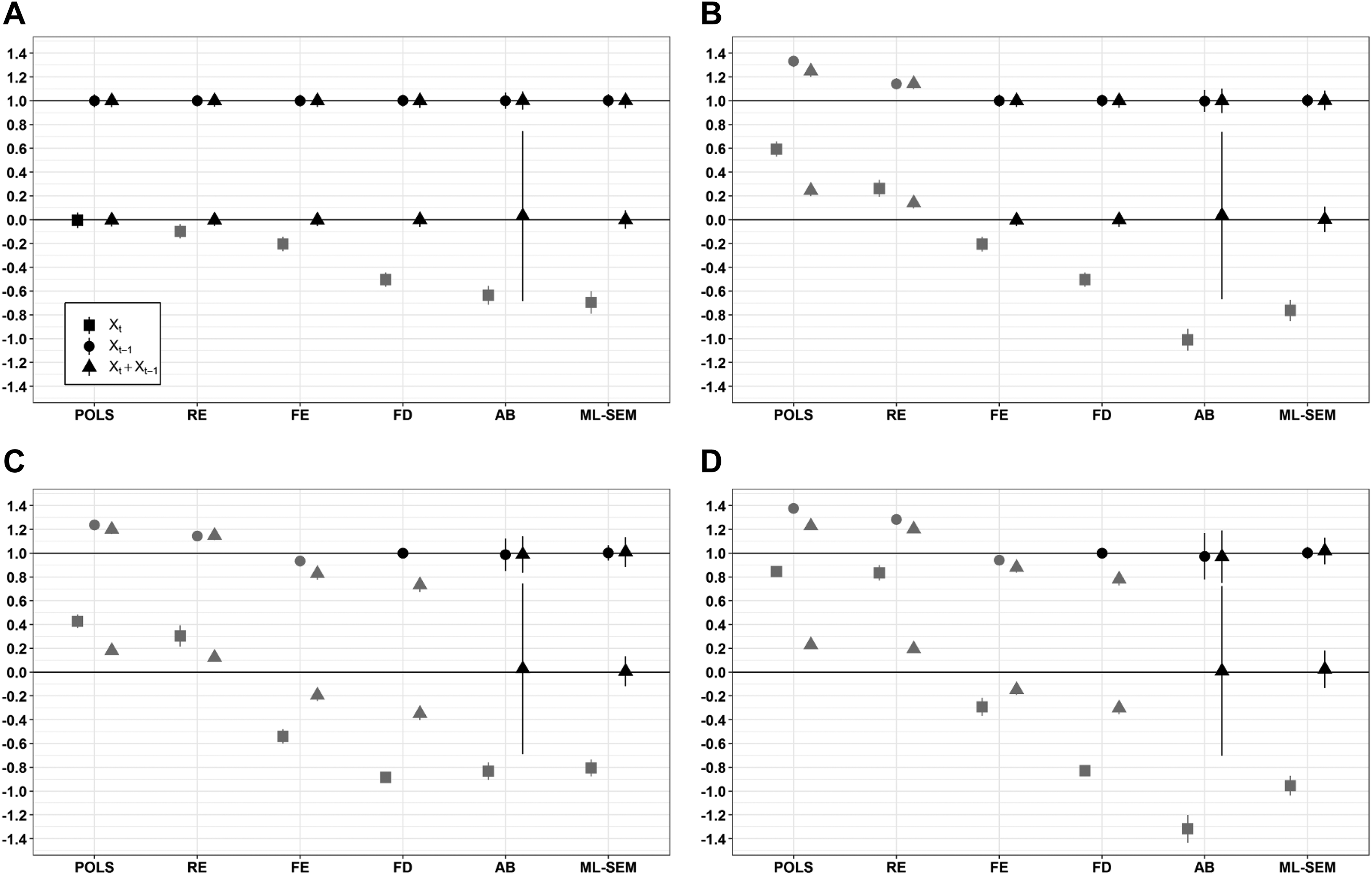
Simulation results for the lagged world (n = 500, t = 5, 500 iterations; 95% confidence intervals). Unbiased estimates are colored in black and biased estimates in gray. The solid horizontal lines represent the true estimates.

In sum, the results confirm that only the AB and ML-SEM model are able to identify the true causal effects of both the lagged and the contemporaneous value of X in all scenarios. Complementing the finding by Vaisey and Miles (2017), the results caution against including (only) a contemporaneous effect in panel models as a default. If the actual causal effect is lagged, only modeling a contemporaneous effect leads to the underestimation of the actual causal effects with coefficients potentially even switching signs.

Mixed World

In the final step, we consider a world in which Y is affected both by the contemporaneous and by the lagged value of X, that is, in which $\lambda =0.5$ and, accordingly, the effects of both $x_{it}$ and $x_{it-1}$ are 0.5. The performance of the different models under such circumstances is important because in many empirical applications both past and current values of X might affect the current outcome. For example, both past and current pay might affect how attractive an occupation is to males and females and thus the current rate of female employees.

Figure 4 shows the results for such a mixed world. In contrast to the previous figures, the graphs include only one horizontal line, at which both effects of 0.5 should be located in case of unbiased estimation. We again address the four different scenarios, in turn, beginning with the simplest one in which neither time-invariant unobserved heterogeneity nor reverse causality are present.

Figure 4.

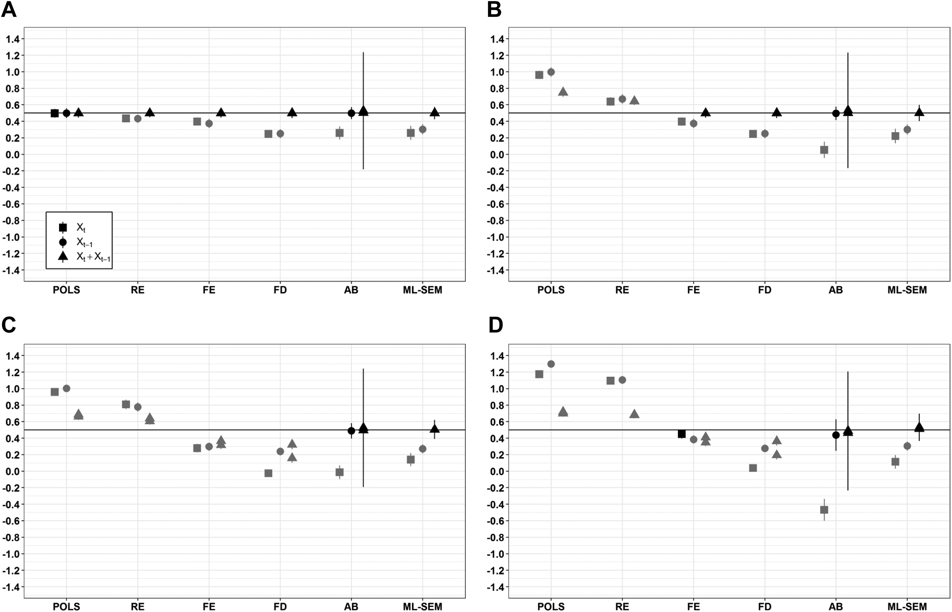
Simulation results for the mixed world (n = 500, t = 5, 500 iterations; 95% confidence intervals). Unbiased estimates are colored in black and biased estimates in gray. The solid horizontal lines represent the true estimates.

Panel A in Figure 4 shows that all six models correctly identify both the contemporaneous and the lagged effect of X, but only if both of them are included in the model. The exception from this pattern is the POLS model, which always correctly identifies the respective effect because of its weaker requirement of contemporaneous exogeneity. In contrast, due to their more demanding assumptions of strict or sequential exogeneity, most other models underestimate the respective effect if only either one of the two effects is included.

Panel B in Figure 4 shows once again that entering time-invariant unobserved heterogeneity induces bias in estimates from POLS and RE models. The pattern mirrors the one of the scenario with a fully contemporaneous effect that we described above, so we do not reiterate it here. Likewise, panels C and D in Figure 4 show that, irrespective of whether or not time-invariant unobserved heterogeneity is present, reverse causality again biases the results not only of the POLS and RE model but also of the FD and FE model. In contrast, both AB and ML-SEM yield unbiased estimates. However, as before, the former model is much less efficient than the latter one.

Robustness Checks

To examine whether our findings are sensitive to sample size, we ran all simulations with n = 100. As the results in Section C of the Online Supplementary show, reduced sample size has little implications for our findings; all results described above hold. Reflecting the loss of statistical power, the only notable yet entirely expectable differences are increased standard errors. This holds true for all models, but especially for ML-SEM.

As a further robustness check, returning to a sample size of n = 500, we varied the length of the panel, considering both less (t = 3) and more (t = 10) points in time. Section D in the Online Supplementary shows that with t = 10—besides more precise estimates—the results are again very similar to those obtained for t = 5.

Section E in the Online Supplementary shows that with t = 3, the results also are very similar to those obtained for t = 5. Again, only the AB model with one effect and the ML-SEM that include both the contemporaneous and the lagged effect of X on Y identify the actual effects in all different scenarios. However, in the most complex scenario that entails both time-invariant unobserved heterogeneity and reverse causality, losses in efficiency are so huge that point estimates are neither significantly different from zero nor from one in most cases. This serves as a note of caution that dynamic panel models might be the right choice in face of reverse causality but are pretty demanding regarding the data. As these robustness checks illustrate, the length of the panel appears to be more important than the number of observations in this regard.

In a final robustness check, we introduced serial correlation by simulating a first-order autoregressive process: ${\epsilon }_{it}=0.2{\epsilon }_{it-1}+{\mu }_{it}$ with ${\mu }_{it}\sim N(0;{\sigma }_{\mu }^2)$ . While previous simulations by Brüderl and Ludwig (2015) highlight that this setup causes severe problems for AB estimators, little is known about how ML-SEM performs under serial correlation. Since ML-SEM also assumes no serial correlation of the errors (see Dynamic Panel Models Allowing for Both Strict and Sequential Exogeneity subsection), it is likely that serial correlation causes problems for this model, too. The results depicted in Section F in the Online Supplementary corroborate this concern, showing that the presence of serial correlation biases results from ML-SEM.

Conclusions and Recommendations for Researchers

This simulation study aimed to provide guidance on how to deal with reverse causality using panel data. After reviewing existing panel models and their key assumptions regarding reverse causality, we assessed their performance under different specifications and a wide range of conditions. Our results demonstrate that frequently used panel models, such as RE or FE models, suffer from biases due to reverse causality, thus being hardly a silver bullet if causal inference is threatened by reverse causality. As also shown, and consistent with Vaisey and Miles (2017), the LFD model is generally better suited to handle reverse causality, but only if the effect of X on Y is indeed fully lagged.

Extending the findings by Vaisey and Miles (2017), we further showed that not only the LFD model, but all considered panel models except for POLS are very sensitive to the correct specification of temporal lags. Our simulation thus reveals that the problem of misspecified lags is rather general, as it also applies to the RE model, the FE model, the AB estimator, and the cross-lagged panel model with FE (ML-SEM). If the effect of X on Y is fully contemporaneous and no lagged effect contributed to the data generating process, all of these models, except for AB, nevertheless yield a statistically significant lagged effect. On the other hand, if the actual causal effect is fully lagged, only modeling a contemporaneous effect all models, including AB, underestimated the actual causal effect with coefficients even switching signs. These findings caution against an unreflected specification of contemporaneous effects in panel models without knowledge about the actual causal process at work. The same holds for using lagged effects as a default.

Our simulation results also show that ML-SEM may help researchers to overcome the problem of misspecified temporal lags. Whereas ML-SEM falls prey to precisely the same lag specification problem as other models, our simulations show that this problem only occurs if ML-SEM includes either a contemporaneous or a lagged effect of X on Y. If both effects are specified, by contrast, ML-SEM provides correct estimates of both effects in all scenarios.

While earlier work has warned researchers what not to do in order to deal with reverse causality (e.g., Brüderl and Ludwig 2015; Vaisey and Miles 2017), our simulation study thus offers guidance on what researchers can do with (at least) three waves of panel data. In short, ML-SEM including both a contemporaneous and a lagged effect of X on Y provides correct estimates of both effects, even in case of reverse causality. If the contemporaneous effect in ML-SEM is negligible, this approach can also serve to justify the application of the LFD model or the AB estimator.

While our simulation results indicate that researchers can rely on ML-SEM to address reverse causality, the method is no panacea either. First of all, it is important to note that our simulation only generated scenarios in which the correct lags are available in the data. While applied empirical research has to make this assumption, more research is needed to explore how ML-SEM and other models perform in cases in which the timing of panel waves does not match the true causal process under investigation. In any case, addressing reverse causality imposes high requirements on the data. Like other panel models, ML-SEM requires a sufficient amount of within variation and at least three panel waves if a lagged effect is included. In addition, ML-SEM contains more parameters to estimate than standard panel models, especially if—as we recommend—both the contemporaneous and the lagged effect of X are specified. While our simulations showed that point estimates are still correct in a setting with three waves and 500 observations, standard errors become so large that it became hard to derive any meaningful substantive conclusions from the empirical results.

Using ML-SEM, further problems can arise that are not directly related to reverse causality but might still limit its usefulness in empirical applications. First, as shown in a robustness check, ML-SEM provides biased estimates in case of serial correlation. Given that serial correlation is rather common using panel data, researchers must be aware of this issue and pay special attention to serial correlation, for example, by directly modeling persistence of variables over time and controlling for variables causing it. Second, ML-SEM requires an iterative algorithm that can fail to converge or can be slow to run (Williams et al. [2018] provide tips for dealing with convergence problems). As shown in Section G in the Online Supplementary, convergence of ML-SEM is not a major issue in simulations with five waves, but it proved to be problematic in shorter panels with only three waves. Furthermore, longer panels (t >10) and unbalanced panels can cause estimation problems; sometimes, switching the software (e.g., to MPlus or R’s lavaan package) might help. Finally, given the rather favorable conditions in our simulation of a simple and systematic data generating process, complete data, and the exclusion of time-varying covariates, additional challenges may also arise in real-world data that contain missing values, nonnormally distributed variables, and interaction effects. Although Moral-Benito et al. (2018) and Williams, Allison, and Moral-Benito (2018) highlight that ML-SEM can use full information maximum likelihood to deal with missing data and also give recommendations on how to deal with nonnormality, it remains open to future research whether our simulation results also hold for such more complex scenarios.

These practical issues aside, our recommendation for researchers facing reverse causality with panel data is straightforward: use ML-SEM to estimate both the contemporaneous and the lagged effect of X on Y. Only this approach yields unbiased estimates of both effects even if reverse causality is present, and it allows solving the problem of misspecified lags that plagues other panel models.

Supplemental Material

Online_Appendix - How to Deal With Reverse Causality Using Panel Data? Recommendations for Researchers Based on a Simulation Study

Online_Appendix for How to Deal With Reverse Causality Using Panel Data? Recommendations for Researchers Based on a Simulation Study by Lars Leszczensky and Tobias Wolbring in Sociological Methods & Research