A Primer on MIMIC Models and Critical Quantitative Methods to Increase Their Use

Abstract

MIMIC (Multiple Indicator and MultIple Causes) models afford powerful claims about measurement—particularly in identifying biased items—and are relatively simple to specify and test. Therefore, we argue that MIMIC models are sorely underutilized and serve important roles in ensuring sound and fair measurement in educational scholarship. When viewed from the perspective of critical quantitative (CritQuant) methodology, MIMICs hold promise in fostering equity-oriented and anti-racist measurement. The MIMIC strategy, employed from a CritQuant perspective, may also reveal how bias in measurement may lead to underestimating the impacts of racism on educational and related outcomes. To increase their use, this primer aims to explain how to specify and evaluate MIMIC models and provides sample code in R (lavaan) and MPlus. The paper concludes by articulating the advantages and disadvantages of MIMICs, from both CritQuant and technical perspectives, to inform educational research.

Introduction

MIMIC (Multiple Indicator and MultIple Causes) models, within a latent variable modeling perspective, afford powerful claims about measurement—particularly in identifying biased items—and are relatively simple to specify and test. It is for these reasons that MIMIC models could play important roles in ensuring sound and fair measurement, particularly in educational scholarship. Given their advantages, we believe that MIMIC models are not utilized as often as they should be. Notably, the aims of MIMIC models often align with a critical quantitative (CritQuant) perspective (delineated from quantitative critical race theory, or QuantCrit; see Fong & Irizarry, 2025; Gilborn et al., 2018) and provide several affordances for critical, anti-racist, and/or equity-oriented measurement. As a brief introduction, CritQuant represents an equity-informed and justice-oriented perspective to quantitative methodology, integrating critical theory(ies) with quantitative methods to advance theory and methodology (e.g., Tabron & Thomas, 2023) that was inspired by Stage’s (2007) perspective of “quantitative criticalism.” (Both CritQuant and QuantCrit are more thoroughly explained later in this paper.) To increase their use and help develop critical quantitative literacy (M. B. Frisby, 2024), this manuscript explains how to specify and evaluate MIMIC models from a technical and critical perspective, as well as provides sample code in R (lavaan) and MPlus. This paper concludes by articulating future directions, from technical and CritQuant perspectives, for MIMIC models to wrestle with.

Simple Model, Complex Claims

Measurement invariance encompasses a broad set of latent variable modeling techniques that probe whether measures function similarly and mean the same thing across groups of interest (Putnick & Bornstein, 2016). Measurement invariance is an important precursor to comparing means, regression coefficients, or other estimates across groups—because unbiased measures are the foundation of fair and precise comparisons of those estimates (Kaplan, 2008; White et al., 2025).

MIMIC models are an approach to measurement invariance, and one that we argue—here and elsewhere (Diemer, Frisby, Marchand & Bardelli, 2025)—is underutilized. MIMIC models are an efficient and powerful way to detect bias in how observed indicators measure latent constructs across groups of interest, or to test for one form of measurement invariance. (We will briefly explain MIMIC models here, and provide much more thorough descriptions later in this paper.) These groups of interest are often social identity groups. For example, MIMIC models can be utilized to examine whether a measure of school engagement functions similarly across adolescent boys and girls. MIMIC models combine aspects of confirmatory factor analyses (CFA) and structural equation modeling (SEM) to test whether groups of interest have (a) similar latent means and (b) similar responses to items, after adjusting for any latent mean differences (Gallo et al., 1994; Kaplan, 2008). Formally, MIMICs test for scalar invariance—whether item intercepts are equivalent across groups when the latent means of those groups have been adjusted for (Gallo et al., 1994). (Scalar invariance is a more rigorous aspect of measurement invariance testing that examines item intercepts, or item means; Putnick & Bornstein, 2016.) Stated another way, after adjustment of latent mean differences, groups should have similar responses to the items that comprise that latent construct (e.g., adolescent boys and girls with comparable latent means on a measure of school engagement should give similar responses to each item assessing how emotionally connected they feel to school ¹ ).

Scalar invariance is considered a “strong” form of measurement invariance that establishes whether the scaling of responses is measured similarly and means the same thing across groups (Putnick & Bornstein, 2016). Following the previous example, if adolescent boys and girls have similar latent means for a school engagement measure, then they should provide a similar response (e.g., 3 = agree) on an item assessing emotional connection to school (see Diemer, Frisby, Marchand & Bardelli, 2025). On the other hand, if responses to items systematically vary across groups, while adjusting for latent mean differences between those groups, then we have evidence of what is known as differential item functioning, or DIF (Kaplan, 2008). To return to the previous example, if gender contributes construct-irrelevant variance to the measurement of school engagement, girls and boys with similar latent means would provide different responses to item(s) measuring emotional connection to school.

In fact, group differences in item means after adjusting for group differences in the corresponding means of the latent variable(s) are precisely how DIF is defined. That is, DIF is an indication of “construct-irrelevant variance” in how an item (or items) measures the latent construct of interest (Finch, 2005). This construct-irrelevant variance is “random error variance or factors that are wholly unrelated to individual differences in the trait measured by the test” (C. L. Frisby, 1999, p. 264). Although DIF is often examined in the item response theory (IRT) tradition (Stark et al., 2006), DIF can more easily be tested in MIMIC models. We therefore focus on the MIMIC approach here.

In a MIMIC specification, this construct-irrelevant variance, or construct bias, predicted by group membership, is evidence that average item responses (either one item or a set of items) vary across the groups of interest being compared. This bias may be systematic and may function to further marginalize or disempower social identity groups if not accounted for. The relatively simple MIMIC specification yields complex claims about group bias in measurement, which makes their underutilization surprising and easily addressable (Diemer, Frisby, Marchand & Bardelli, 2025). The first aim of this paper is to increase the use of MIMICs by providing a primer on their specification and interpretation, as well as noting limitations and future directions for MIMICs to resolve—for the more advanced user—to guide educational research.

Three Steps in Specifying and Testing MIMIC Models

The specification and testing of MIMIC models is relatively simple and can be partitioned into three sequential steps (see also Diemer, Frisby, Marchand & Bardelli, 2025). MIMIC models can be examined in several software packages (e.g., R/lavaan, Stata, MPlus, SAS), with results obtained from different packages highly convergent (Chang et al., 2020; Diemer, Frisby, Marchand & Bardelli, 2025). These three steps are visually represented in Figure 1; a visual representation of a sample MIMIC model is included in Figure 2, and both will be more thoroughly explained later.

Figure 1.

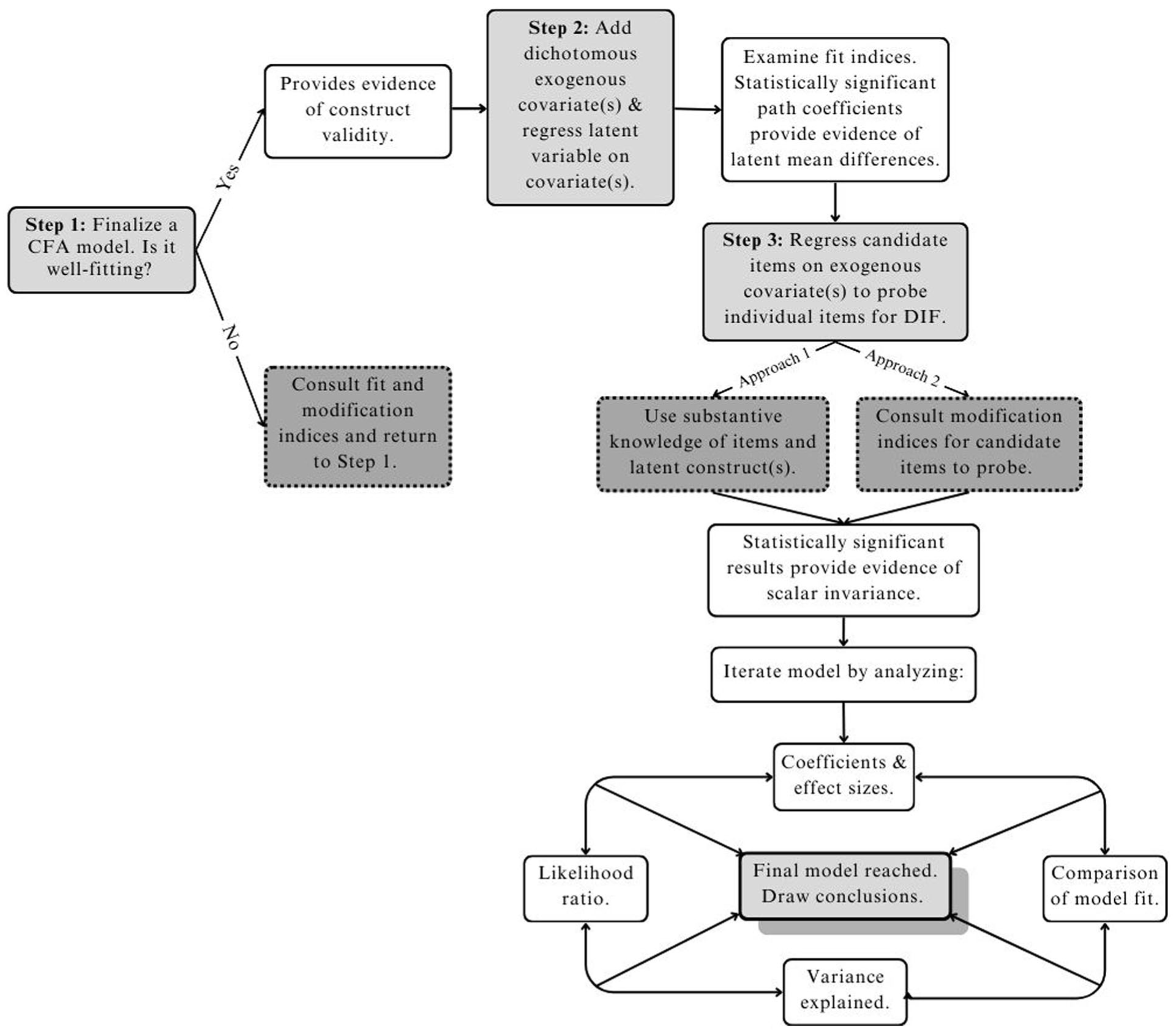
MIMIC Model Flowchart.

Figure 2.

Measuring Tallness and Testing for DIF with a MIMIC Model.

The first step requires a well-fitting CFA model, which allows for the confirmation of a hypothesized factor structure. Stated another way, CFA models serve as a rigorous test of a factor structure to ensure that observed items measure the proposed latent construct well (Kline, 2016). Fit indices such as RMSEA, CFI, TLI, and SRMR are reported and compared to commonly agreed cutoffs to determine if the data are a good fit to the model and if items load significantly and with sufficient magnitude onto their specified latent construct. It is important to ensure at this initial step that observed indicators are normally distributed. This can be done by examining levels of skewness and kurtosis (Kline, 2016). If it is revealed that the data are non-normal, there are options on how to proceed. Depending on the extent of non-normality, an alternative estimator such as MLR (maximum likelihood with robustness to non-independence and non-normality) can be specified in the CFA model, and/or non-normal variables may need to be transformed (Kline, 2016, pp. 77–81). During the CFA, modification indices may be reviewed to determine if any error covariances are related. These error covariances may be modeled in the CFA to improve fit if they can be substantively justified. For further approachable treatments of CFA analyses, see Kline (2016) and Furr (2021). ²

The second step of MIMIC modeling incorporates aspects of structural equation modeling in that an exogenous covariate is specified as a predictor of the latent mean of the latent variable. Groups to be compared are traditionally specified as dichotomous contrasts in the exogenous covariate (e.g., following the example from earlier, boys = 0 and girls = 1). The 0 group in the covariate serves as the comparison or reference group in the interpretation of parameter estimates; the 1 group is the focal group that is “in comparison” to the 0 group (Chang et al., 2020; Ro & Bergom, 2020). This covariate is exogenous in that it is “on the outside”—nothing else in the model predicts it (represented in a figure, no arrows go into the exogenous covariate, yet arrows originate from the covariate into other parts of the figural model—see Figure 2 for an example that will be more thoroughly explained later). The covariate itself predicts the latent mean (as noted previously) and individual items (to be reviewed later). The analyst takes note of any significant latent mean differences (i.e., does the exogenous covariate significantly predict the latent mean?) and whether model fit increases, or decreases, via the variance explained by the path from the covariate to the latent variable. (Note: a significant latent mean difference is not required for model fit to increase or decrease). A statistically significant latent mean difference provides evidence of a difference in latent means across the two groups that comprise the exogenous covariate. A nonsignificant latent mean difference indicates there is no evidence of a significant latent mean difference across the two groups that comprise the exogenous covariate. Independent of whether this path is significant or not, one would proceed to the next step of MIMIC modeling.

Importantly, this path from the exogenous covariate to the latent mean from step two must be retained in the subsequent third step. This path has the effect of adjusting for or “controlling away” (similar to adjusting for other variables in a multiple regression analysis) latent mean differences across the groups of interest; adjusting the means of groups is required to test whether individual items differ. Otherwise, any detected differences in the items may simply reflect unadjusted latent mean differences that are manifesting in the observed items (Kaplan, 2008). This is an important component of the MIMIC modeling process, and we elaborate with an illustrative example later in this primer.

The third step retains the regression of the latent variable onto the exogenous covariate while also regressing individual items onto the covariate. This step tests scalar invariance (i.e., item intercepts in the case of continuous variables or thresholds in the case of categorical variables are invariant across groups in the exogenous covariate). Item(s) that are significantly predicted by the exogenous covariate, while adjusting for latent mean differences, demonstrate non-invariance (i.e., difference or heterogeneity) in their item intercepts at the scalar level. Stated another way, this third step tests for DIF, or differential item functioning, which indicates biased items (in that biased items suggest group differences in responses even when latent mean differences have been adjusted for; see Finch, 2005). Scalar non-invariance entails that the response scaling of items functions differently across groups. In practical terms, groups with a similar latent mean should provide a similar response to an observed item. In contrast, when DIF is present (or in this case, scalar non-invariance), one group systematically endorses items at a higher level than the other group, even when those groups have similar latent means.

This third step begs a procedural question: Which observed items should be regressed onto the exogenous covariate? This can be a thorny decision, particularly when many observed items can be tested. Testing too many items inflates the risk of “false positive” Type I errors and/or risks model under-identification. Two approaches, which are not mutually exclusive, guide the selection of observed items to probe for DIF. First, substantive considerations may suggest item candidates. For example, knowledge of gendered differences in inhibition may suggest testing for DIF in items that measure inhibition on an executive function scale.

The second approach uses candidate items generated by modification indices (MI), provided by many software packages. MIs use Lagrange multipliers to identify empirical modifications to a model to reduce overall chi-square value (scaled such that larger values suggest worse fit) and thereby improve model fit (Muthén & Muthén, 1998-2017). Yet, this stands at odds with a canonical idea in latent variable modeling: Avoid only using empirical criteria to guide post-hoc model modifications, without attending to substantive theory (Kline, 2016).

There is one notable exception: Experts argue for using MIs to identify candidate items to test for DIF in MIMIC modeling (e.g., Gallo et al., 1994; Kaplan, 2008; Muthén & Muthén, 1998-2017). This is standard practice in the MIMIC modeling tradition (e.g., Chang et al., 2020; Diemer, Frisby, Marchand & Bardelli, 2025; Montoya & Jeon, 2020). Practically, this entails scrutinizing the MI section of software output and taking note of items that are associated with the exogenous covariate. For example, the MIs may suggest regressing an item about emotional connection to school on the exogenous gender covariate. (Alternatively, the MIs may suggest a correlation between an item and the covariate or instead regressing the covariate on the item; any meaningful such “signal” in the MIs merits testing for DIF). The analyst would then make the post-hoc model modification(s) suggested by the MIs to probe for DIF. If multiple items are implicated by the MIs, we would suggest testing for DIF sequentially, one item at a time, for simplicity and clarity. The utility of MIs is underscored by item impact examinations in large-scale achievement tests, where items may demonstrate adverse (empirical) impact across racial groups despite seemingly benign item content with no readily apparent bias (Kidder & Rosner, 2002). From a CritQuant perspective, fully explained later in this paper, there are important equity implications for testing for DIF.

Readers may wonder whether it’s necessary to explore DIF if they have a well-fitting CFA model. To address this, we note that the goal of a latent variable model, like other regression-based methods, is to explain variance among the observed variables. A key aspect of how model fit indices are calculated is how well the specified model explains variance, in comparison to other plausible models (Hu & Bentler, 1999). The introduction of exogenous variables presents new candidate variables to explain the variance in the latent variable(s) and corresponding items. Accordingly, model fit may change when these variables are introduced.

Note that relationships between exogenous covariates and items are assumed to be zero unless explicitly modeled otherwise. However, MIs may detect exogenous covariates that can account for item-level variance beyond what variance is already accounted for by the latent variable. If covariate-item relationships exist but are unmodeled, fit indices will generally decrease—because they are based on maximizing the variance accounted for. Said another way, if there is any meaningful amount of variance “left on the table” that could be explained by adding relationships between the newly included covariate(s) and observed items, fit indices will decrease accordingly. (Technically, the amount of variance explained must be of sufficient magnitude to merit the degree(s) of freedom each path requires from the covariate to an item(s).)

In this way, the well-fitting model established in the first CFA step may not extend to the second and third steps, once covariates are included. Further, the change in model fit will be determined by how much additional item-level variance is explained by the covariates, over and above mean differences in the latent construct. If, however, the model fit remains satisfactory after including covariates in the model, substantive considerations to probe for DIF should be used in place of modification indices. One caution is in order here: very well-fitting models may have a chi-square value small enough that modification indices cannot suggest how to improve the model by estimating relationships between the covariate and observed items.

Practically, the analyst would add the tests for DIF to their code file, reanalyze the model, and take note of changes in model fit (e.g., does fit improve as new variance in the items is accounted for by the covariate? Or is the new variance accounted for outweighed by the loss in degrees of freedom additional paths entail?) as well as the significance of paths from the covariate to the observed item(s). Again, significant regression(s) of the observed item(s) onto the covariate, after adjusting for latent mean differences, is evidence of DIF or scalar non-invariance.

Addressing DIF

Identifying DIF begs the question of how to address DIF. The magnitude of DIF is an important consideration in determining how to address it. However, the psychometric literature does not provide clearly agreed upon standards for judging the magnitude of DIF, in contrast to Cohen’s (2013) classification of generally agreed upon effect size estimates for multiple regression (e.g., small effects where β = .10, medium where β = .30, and large where β = .50). Kraft’s (2020) updated classification for educational research are more informative, wherein effect size estimates are often smaller than those obtained by Cohen in social psychological and highly controlled lab studies—and thus updated so that less than .05 (in SD units) is small, .05 to less than .20 is medium, and .20 or greater is large.

Absent those standards for MIMIC models, estimating the amount of variance explained in an item intercept provides one way to understand the magnitude of DIF. Squaring the standardized regression coefficient between an exogenous covariate and an observed item yields an estimate of variance explained in the item intercept by the exogenous covariate, after adjusting for latent mean differences. For example, a γ of .30 between an exogenous covariate and an observed item yields an estimate of 9% of variance explained in the item intercept by that exogenous covariate. While this may seem like a relatively modest amount of variance, γ = .30 is understood as a “large” effect in the Kraft (2020) classification, and 9% of variance can have important practical or clinical implications. A related concern is that tests for DIF can be substantially overpowered with very large samples, obtaining statistical significance for tests for DIF that are not meaningful or practically significant, as is broadly true in other tests of statistical significance (Cohen, 2013; Kraft, 2020).

After considering the magnitude of DIF, three approaches to addressing DIF can be taken. The first option would be to revise an item or items that exhibit DIF. These revisions would be taken with a substantive understanding of how the exogenous covariate may relate to the item content. For example, if gender serves as the exogenous covariate in a MIMIC model, and the item content contains gendered processes, sexism, or related substantive content, then the item content could be revised to attempt to mitigate or remove that gender-based DIF. After revising the item or items exhibiting DIF, those items could be administered to a new sample, and whether the revised items also exhibit DIF would be empirically examined in a new MIMIC model.

The second approach to addressing DIF is to simply remove the offending item or items exhibiting DIF. From an equity perspective, this would provide a fairer measure and is the most straightforward way to address DIF. On the other hand, it may be difficult to remove items from short measures because a shorter measure generally provides less coverage of key facets and content of the latent construct of interest (Furr, 2021).

The third approach to addressing DIF is only available in a structural equation modeling (SEM) specification. As noted in the previous review of the steps of MIMIC modeling, retaining the path from the exogenous covariate to the latent variable (step two) has the effect of adjusting for or “controlling away” any latent mean differences between the groups in the covariate. Similarly, retaining the path from the exogenous covariate to the latent variable and to the observed item (step three) has the effect of controlling away latent mean differences as well as item mean differences (i.e., item intercepts), or DIF. In a SEM model, retaining these paths would adjust for DIF in item intercepts while estimating the role of that latent variable as a predictor and/or outcome in a full SEM model (Gallo et al., 1994). Stated another way, this approach would provide estimates of how latent variables relate to each other, with the impact of item-level DIF mitigated in those estimates.

Given these options, the user can now recursively refine the model shown in Figure 1. This can be done by analyzing likelihood ratios, comparing the model fit of various iterations of the model, scrutinizing coefficients to characterize the magnitude of DIF, and obtaining variance explained by squaring standardized coefficients between the exogenous covariate and observed item(s) as a way to calculate r-squared values. This step must be done with caution and guided by substantive knowledge of the constructs in order to avoid p-hacking (e.g., re-running analyses until a desired relationship is detected). Upon completing these analyses, a final model will be obtained, and appropriate conclusions can be made.

This capacity to detect item bias is a powerful feature of MIMIC models, and one with important equity implications, which are more thoroughly considered later in this paper from a critical quantitative perspective. Before doing so, we provide a simplified example of this process to better illustrate the three steps in MIMIC models.

Simplified Example of the Three Steps: Tallness

We turn to examine hypothetical gender differences in sixth-grade “tallness” measures to illustrate the three steps in testing a MIMIC model; please see Figure 2. In this (artificial) example, the iPhone measure app, wall chart, tape measure, and self-reported height of four observed measures of the latent variable tallness. Standardized factor loadings for these four observed indicators—.68, .85, .79, .74, respectively, often notated as lambda, or λ₁, λ₂, λ₃, λ₄—represent how well each indicator measures the latent construct of tallness. Assuming satisfactory model fit, this achieves step one, establishing a well-fitting CFA model. If model fit is not satisfactory, the CFA model should be modified until satisfactory—or abandoned.

Step two in the MIMIC process regresses the latent variable onto the exogenous covariate. As depicted in Figure 2, the .23 standardized regression coefficient (often notated as gamma, γ) from the exogenous covariate, gender, to the tallness latent variable reflects a significant latent mean difference. Girls are on average taller than boys in sixth grade, which would correspond to a latent mean difference in tallness (the latent variable here). In this case, girls, who are the 1 group or focal group in the covariate, have a significantly higher latent mean for tallness than boys, who are the 0 or comparison group in the covariate.

From an equity perspective, we would not problematize these latent mean differences, in that they simply reflect differential rates of maturation and growth. If we adjust for the latent mean differences in tallness for boys and girls, our four observed measures should yield (on average) similar measurements of height for girls and boys—because we’ve adjusted for the latent mean of tallness, the observed instruments should yield similar measurements of height. At the very least, after adjusting for latent mean differences, our observed measures should be unrelated to the exogenous covariate. On the other hand, if we adjust for the latent mean of tallness for girls and boys, but the observed measures consistently yield (on average) measurements of height that are significantly different for girls (or boys), then we would have an example of a biased observed indicator; in our example, it is self-reported height. It stands to reason that boys might overreport their height. In this example, either substantive considerations (e.g., boys might be motivated to overreport their height and/or girls might underreport their height) or model modification indices could identify candidate items to test for DIF in the subsequent step three of the MIMIC modeling process, to which we now turn our attention.

Step three of the MIMIC modeling process regresses candidate observed items onto the covariate, while retaining the regression of the latent variable onto the covariate from step two. This is reflected in Figure 2 by the −.30 standardized regression coefficient, which again is often notated by gamma (γ), from the exogenous covariate (gender) to the self-reported height observed indicator. This coefficient is interpreted in comparison to the 0 or comparison group in the exogenous covariate; in this case, girls are the 1 or focal group, so the coefficient is interpreted for girls in comparison to boys (Ro & Bergom, 2020). Interpretively, the −.30 value entails that tallness is over-measuring self-reported height for girls, or that after adjusting for the latent mean of tallness for boys and girls, girls have systematically higher scores on the self-reported height item than boys do. Informed by the above, squaring this coefficient indicates that 9% of the variance in the self-reported height item intercept is explained by the gender exogenous covariate. The addition of the statistically significant and negative DIF path downwardly adjusts for this overmeasurement. This is evidence of scalar non-invariance (i.e., intercepts) or that the scaling of the self-reported height item varies between girls and boys. This scalar non-invariance is evidence of DIF in the self-reported height item.

To address DIF in this item, it may be possible to revise the item and readminister it, in an attempt to remove DIF from the item. In this case, however, it appears simpler to remove the self-reported height item and only use the other three items with no indication of DIF. If the tallness latent variable was used as a predictor or outcome variable in a SEM specification, then retaining the paths from the gender exogenous covariate to the tallness latent variable and from the exogenous covariate to the self-reported item would have the effect of “controlling away” or adjusting for item-level DIF in SEM models.

Importantly, if we did not adjust for latent mean differences in tallness between boys and girls in step two, our four observed measures would yield (on average) under-measurements of height for girls, in comparison to boys. This is because all items are positively adjusted by a factor of .23—the positive latent mean adjustment in tallness for girls, given by γ —multiplied by each item’s factor loading (see Figure 2). We would not consider self-reported height to be producing biased measurements of height in this example—self-reported height might be simply capturing overall, unadjusted differences in the tallness latent variable, yet manifesting in the observed items. This illustrates, hopefully, the importance of adjusting for latent mean differences when evaluating group differences in the observed items within MIMIC models.

Mathematical Representation of MIMIC Models

Having aimed to make the process, specification, and interpretation of MIMIC models more straightforward by walking through the three steps and a figural example, we pivot now to the mathematics and notation underlying MIMIC models. The mathematical machinery of MIMIC models can be illustrated through expressions for measurement and structural equation models for latent variables (Kline, 2016). The measurement model, as evaluated by CFA, for an endogenous latent variable η can be written as

$$y={\mathrm{\Lambda }}_y\eta +ϵ$$

where y is a vector of indicators (e.g., self-reported height, tape measure, wall chart, and measure app), Λ_y is a matrix of factor loadings for each indicator (e.g., .68, .85, .79, .74), η is vector of latent endogenous variables (e.g., tallness), and ∈ is a vector of residual terms for each indicator in y. We can express each indicator y_k in terms of simple linear regression equations

$$\begin{array}{c}{y}_{1i}={\lambda }_1{\eta }_i+{ϵ}_{1i}\hfill \\ y_{2i}={\lambda }_2{\eta }_i+{ϵ}_{2i}\hfill \\ y_{ki}={\lambda }_k{\eta }_i+{ϵ}_{ki}\hfill \end{array}$$

where k is the number of observed indicators for the endogenous latent variable η, and i refers to the response from individual i in the overall sample size n. In the previous example, k = 4 indicators (self-reported height, tape measure, wall chart, and measure app). Important to DIF, each y_k is modeled exclusively by its relationship to η in the measurement model, when conducting CFA. In other words, there are no covariates in the measurement model. For notational ease, we assume each y_k is mean-centered and therefore takes zero for its intercept. Accordingly, it is not explicitly written above, but implicitly present as γ₀ = 0.

Covariates such as gender are added after obtaining a satisfactory CFA model. However, adding covariates changes the measurement model to a structural model and is written as

$$\eta =\mathrm{B}\eta +\mathrm{\Gamma }\xi +\zeta$$

where η is the same vector of endogenous latent variables as in the measurement model, Β is a matrix of regression coefficients relating the endogenous latent variables in η to one another, ξ is a vector of exogenous variables (e.g., gender), Γ is a matrix of regression coefficients relating the exogenous and endogenous variables (e.g., γ = .23), and ζ is a vector of residuals for the endogenous variables in η. For simplicity, we assume a model such as the one shown in Figure 2 that has no structural paths (regressions) between multiple endogenous variables, though the previous equation can accommodate more complicated models in the assessment of DIF. This assumption allows the matrix Β to be zero and leaves only the $\mathrm{\Gamma }\xi +\zeta$ part of the structural equation. For the sake of generality, we take an arbitrary ξ₁ as our exogenous covariate, but the reader can mentally substitute something more concrete, such as gender or age. Combined with the structural model, this results in a simple regression model for predicting an arbitrary endogenous latent variable η₁

$${\eta }_{1i}={\mathrm{\gamma }}_1{\xi }_i+{\zeta }_{1i}$$

Now suppose, without loss of generality, that y₁ is the indicator we wish to evaluate for DIF. Substituting the equation above for η₁ into the equation for y₁, we get that

$$\begin{array}{c}{y}_{1i}={\lambda }_1{\eta }_i+{ϵ}_{1i}\hfill \\ ={\lambda }_1\left({\mathrm{\gamma }}_1{\xi }_{1i}+{\zeta }_{1i}\right)+{ϵ}_{1i}\hfill \\ ={\lambda }_1{\mathrm{\gamma }}_1{\xi }_{1i}+{\lambda }_1{\zeta }_{1i}+{ϵ}_{1i}\hfill \end{array}$$

In this expression, the indicator y₁ is affected by ${\xi }_1$ indirectly and solely through the relationship between ${\xi }_1$ and η₁. Said another way, the observed indicator (y₁) is predicted by the endogenous latent variable (η₁), which is predicted by an exogenous covariate $({\xi }_1).$ This is similar to a mediation model in which the direct effect—the DIF path—is fixed to zero. Expressed this way, we implicitly assume that after controlling for the relationship between ${\xi }_1$ and η₁, the relationship between ${\xi }_1$ and y₁ is nil. Analogous to the “tallness” example mentioned earlier, this assumes the relationship between gender and self-reported height equals zero. It is precisely when this relationship is significant and nonzero that we have evidence of DIF. We write this relationship as

$$\begin{array}{c}{y}_{1i}={\lambda }_1{\eta }_{1i}+{\mathrm{\gamma }}_2{\xi }_{1i}+{ϵ}_{1i}\hfill \\ ={\lambda }_1\left({\mathrm{\gamma }}_1{\xi }_{1i}+{\zeta }_{1i}\right)+{\mathrm{\gamma }}_2{\xi }_{1i}+{ϵ}_{1i}\hfill \\ ={\lambda }_1{\mathrm{\gamma }}_1{\xi }_{1i}+{\lambda }_1{\zeta }_{1i}+{\mathrm{\gamma }}_2{\xi }_{1i}+{ϵ}_{1i}\hfill \end{array}$$

This final equation is identical to the equation without DIF, but with the addition of the ${\mathrm{\gamma }}_2{\xi }_{1i}$ term (which is the only term pertinent to our discussion of DIF). Whenever γ₂ is nonzero, this term adjusts the intercept of y₁ by a factor of ${\mathrm{\gamma }}_2{\xi }_1$ . Whenever this term is nonzero and statistically significant, we say that we have evidence of DIF. Thus, whenever ${\xi }_1$ is a dichotomous variable, ³ such as the binary boy/girl used in our example, the value γ₂ is added to the intercept whenever ${\xi }_1$ takes the value of 1. In both cases, however, the statistical significance of γ₂ is what constitutes DIF, and its impact on the intercept of the regression model is what corresponds to “strong” or “scalar” non-invariance from a measurement invariance perspective.

Having established the procedural, notational, mathematical, and graphical basis for MIMIC model specification and interpretation, we pivot toward an empirical example of MIMIC models, using the National Longitudinal Study of Adolescent to Adult Health study, more commonly known as Add Health (Harris, 2013).

Empirical MIMIC Example: Everyday Discrimination Scale

We apply MIMIC modeling to Add Health study data (Harris, 2013) to further illustrate the “how to” of MIMICs. Wave V of Add Health surveyed a longitudinal panel of adults between the ages of 32–42 during the years 2016–2018; from this larger data collection, we focus on the widely used Everyday Discrimination Scale (EDS, Sternthal et al., 2011). We examine a subsample of (N = 3,660) Wave V respondents who identified as Black (N = 863, 23.57%) or as white (N = 2,797, 76.42%). This focus on two specific ethnic/racial groups is motivated by an interest in using MIMIC modeling to examine racial differences in how people who self-identify with different ethnic/racial groups respond to items assessing racialized experiences, consistent with a CritQuant perspective, which will be carefully considered.

Following the three-step approach, we first fit a CFA to these data (step one), and then probe whether white and Black participants had different latent means on this Everyday Discrimination Scale (step two), and finally probe for items exhibiting DIF (step three), detailed next. (These data, along with accompanying code in Mplus and R (lavaan package), are available as supplementary material, via the OSF link (https://osf.io/ncbuw/files?view_only=53068840ba3941cfb0b84744066a704a), as well as via the ICPSR repository (https://doi.org/10.3886/E238041V1) (Diemer, Frisby, & Marchand, 2025). Please also see the annotated output file in Supplementary Materials, which is intended to explain and elaborate on the MIMIC modeling process.

Everyday discrimination refers to the daily hassles, microaggressions, and interpersonal discrimination that people of color face and is distinct from structural- and historical-level forms of racism, such as redlining and racialized wealth disparities. This conceptualization is consistent with Helms’s (2006) Individual Differences and other critical perspectives (e.g., White et al., 2025) that interrogate the manifestation of structural racism and anti-Blackness in everyday interactions. This harmonization of critical theory and quantitative methodology reflects critical quantitative principle #1, a foundation of critical theory and quantitative methodology (Diemer, Frisby, Marchand & Bardelli, 2025).

The five-item short version of the Everyday Discrimination Scale (EDS) has been widely used and assesses the frequency of discriminatory experiences in day-to-day life (Sternthal et al., 2011). All items were on a four-point Likert scale ranging from (1) never to (4) often. Items were coded such that higher scores correspond to more frequent discrimination. A sample item reads “You receive poorer service than other people at restaurants or stores.” Estimates of internal consistency with the original sample were α = .77; we obtained estimates of α = .74 and a mean inter-item correlation of .37 with this Add Health subsample.

Following step one, we first subjected these five items to a CFA, using maximum likelihood (ML) estimation. The first item loading was freely estimated, and the latent variance was fixed to one for model identification purposes. This CFA provided a good fit to the data (CFI = .99, TLI = .97, RMSEA = .05, SRMR = .02; Hu & Bentler, 1999); the magnitude of item loadings was strong, and all items loaded significantly. Item stems, internal consistency estimates, and factor loadings are included in Table 1.

Table 1

Confirmatory Factor Analysis: Everyday Discrimination

Factor and Items	Standardized Loadings
Factor 1: “Everyday Discrimination” (α = .74; mean inter-item correlation = .37)
In your day-to-day life, how often have any of the following things happened to you?
1. You are treated with less courtesy or respect than other people.	.69*
2. You receive poorer service than other people at restaurants or stores.	.65*
3. People act as if they think you are not smart.	.72*
4. People act as if they are afraid of you.	.45*
5. You are threatened or harassed.	.52*

Model fit indices: CFI = .99, TLI = .97, SRMR = .02, RMSEA = .05.

Note. *denotes statistical significance at p < .05.

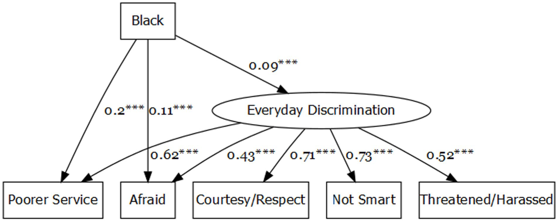
In step two, an exogenous covariate was added to the existing CFA model. White respondents served as the 0 or “reference” group and Black respondents as the 1 or “focal” group in the exogenous covariate, which is labeled Black in Figure 3. The path from the Black covariate (the topmost square in Figure 3) to the everyday discrimination latent variable (circle) was statistically significant, such that Black respondents were more likely than white respondents to report everyday discrimination (β = .09, p < .001). In other words, the everyday discrimination latent construct exhibited statistically significant mean differences by respondent racial/ethnic identity, in expected directions. However, we would have expected a larger difference in the latent mean, given that white people do not experience racialized everyday discrimination. Importantly, if we did not adjust for differences between Black and white respondents in the latent mean of the Everyday Discrimination Scale (EDS), the five EDS items would yield (on average) under-measurements of everyday discrimination for Black respondents, in comparison to white respondents. This is because all items are positively adjusted by a factor of .09—the positive latent mean adjustment in everyday discrimination for Black respondents, given by γ—multiplied by each item’s factor loading (as depicted in Figure 3).

Figure 3.

MIMIC Model, Everyday Discrimination Scale.

In step three, observed indicators that measure the latent construct are regressed onto (or are predicted by) the exogenous covariate. In Figure 3, these are the paths from the Black exogenous covariate to the “poorer service” and “afraid” observed items. These two items were selected based on substantive theory, as we expected these two items may function differently for people who identify as white than for people who identify as Black, given the histories of racialized daily hassles, microaggressions, and stereotyping that Black people encounter (e.g., Helms, 2006; Randall, 2021). Each of these paths represents a formal test for DIF, or whether the intercepts of these items are equivalent across the groups in the exogenous covariate, after adjusting for latent mean differences in the previous step two.

Black respondents reported experiencing poorer service in restaurants or stores more frequently (β = .20, p < .001), and Black respondents reported that other people more frequently act afraid of them (β = .11, p < .001), even after adjusting for the greater latent mean level of everyday discrimination of Black respondents. According to Kraft’s (2020) updated effect size taxonomy for educational research, these would correspond to “medium” effect sizes. However, we note that these effect size estimates were derived from observational data, rather than a fully randomized RCT, and thus these estimates of effect size are likely biased upward (i.e., inflated; see Kraft, 2020).

Each of these statistically significant paths provides evidence of DIF—in other words, they do not meet the criteria for scalar invariance (i.e., are non-invariant). Stated another way, scalar invariance indicates that the intercepts are similar across groups or that the scaling of items is measured in the same way and means the same thing across groups of interest (Putnick & Bornstein, 2016). In this case, after adjusting the latent means to be similar for Black and white respondents, the item intercepts (i.e., item means) should also be similar. Further, we see that Black respondents report higher levels of racist experiences in these two items (as evidenced by the .20 and .11 coefficients), even after adjusting the EDS latent means to be similar (by .09) for Black and white respondents. The EDS items are keyed such that higher responses indicate more everyday discrimination experiences. This indicates these two items are biased in that they under-measure everyday discrimination for Black respondents—surprising in a measure explicitly developed to capture discrimination, particularly the discriminatory experiences that Black people face (Sternthal et al., 2011). The MIMIC of the Everyday Discrimination Scale showed the promise of this approach in that it identified items that under-estimate discrimination for people who identify as Black. (The positive coefficients make interpretation a little more complex, but in this case, they indicate that these two items under-measure the degree of discrimination Black respondents experience and thus need to be increased, because the EDS items are keyed such that higher scores represent more discrimination). From a substantive perspective, this is important because of well-established links between racialized discrimination and educational as well as other outcomes among people of color (see Sternthal et al., 2011). For example, it is well-established that racial discrimination from teachers and school personnel is negatively associated with Black students’ motivation and achievement (Castillo & Strunk, 2025; Randall, 2021). Alternatively, it is established that Black women educators with similar effectiveness ratings as white women will nevertheless be rated lower (Campbell, 2023). More specifically, the under-measurement of racialized discrimination in the Everyday Discrimination Scale may lead to downward bias in estimates of the relations between discrimination and outcomes among Black respondents.

This empirical example also illustrates the three steps of MIMIC modeling depicted in Figure 1 and reviewed previously, intending to clarify how educational researchers can employ MIMIC modeling. It also reveals how bias in measurement may lead to underestimating the impacts of racism on educational outcomes. Both are pertinent for using MIMIC models with the aim of developing critical quantitative literacy (M. B. Frisby, 2024). To this end, we now more fully explain the critical quantitative (CritQuant) perspective to further illustrate the affordances of MIMIC modeling and its limitations, from critical quantitative and technical perspectives.

Critical Quantitative Methodology

CritQuant is a critical approach to quantitative methodology and the research enterprise. That is, what research questions are asked and how those questions are pursued is what characterizes CritQuant (Tabron & Thomas, 2023). For example, quantitative studies of critical consciousness (e.g., Bañales et al., 2020; Diemer & Blustein, 2006) and analyses of administrative data in support of the Mexican-American studies program (Cabrera et al., 2014) represent enactments of CritQuant by “calling out and challenging racist systems with rigorous quantitative research design and application,” which can enhance the ability of educational research to be anti-racist (Diemer, Frisby, Marchand & Bardelli, 2025, p. 372). Garvey et al. (2019) illustrate applications of CritQuant to examine how gender is conceptualized and measured in survey research, grounding their work in critical feminist and queer theories.

Recent work (Diemer, Frisby, Marchand & Bardelli, 2025) articulates five guiding principles of CritQuant, integrating ideas from scholarship variously labeled as “quantitative criticalism” (Arellano, 2022; Hernández, 2015; Stage, 2007; Stage & Wells, 2014), “social justice-oriented methodology” (Cabrera & Chang, 2019; Cokley & Awad, 2013), “critical quantitative intersectionality” (Jang, 2018), and ideas from quantitative crit (QuantCrit; Castillo & Gillborn, 2023; Gilborn et al., 2018). Before more fully elaborating CritQuant, it is important to first delineate CritQuant from QuantCrit; the latter being a more formalized and paradigmatic instantiation of critical race theory with quantitative methodologies.

Delineating CritQuant from QuantCRiT

Castillo and Gillborn (2023) define quantitative critical race theory (QuantCrit) as “a rapidly developing approach that seeks to challenge and improve the use of statistical data in social research by applying the insights of Critical Race Theory (CRT)” (p. 1). QuantCrit is a specific enactment of the five central tenets of critical race theory (e.g., whiteness as property, the endurance of racism) via quantitative methodology (Fong & Irizarry, 2025; Gilborn et al., 2018). QuantCrit can be illustrated by a sample enactment of the research process, reframing the research question of “Why are Black boys expelled from our schools at a higher rate than other boys?” to instead be “Why do schools expel disproportionate numbers of Black boys?” (Castillo & Gillborn, 2023, p. 5). A systematic review of QuantCrit research can be found in Castillo and Babb (2023), and its implications for educational psychology were recently delineated in Fong and Irizarry (2025).

The specific alignment of CRT with quantitative methodology is a core strength of QuantCrit (Castillo & Strunk, 2025; Gilborn et al., 2018). It differs from CritQuant in important ways. One of these ways is the alignment with a specific critical theory—CRT—whereas CritQuant takes its inspiration from quantitative criticalism (Stage, 2007). Although quantitative criticalism is specifically rooted in critical theory derived from the Frankfurt School, CritQuant is not rooted in one specific critical theory. Instead, CritQuant is guided by the notion that different research questions (e.g., What are the impacts of ethnic studies curricula on minoritized students?) are best animated by critical theories that align tightly with those substantive questions and/or identities. For example, Garvey et al. (2019) interrogate how gender is conceptualized and measured in survey research, animated by critical feminist and queer theories, which would be less theoretically compatible with the CRT theory guiding QuantCrit. We refer the reader to a recent work by Tabron and Thomas (2023) for a more comprehensive delineation between these frameworks.

CritQuant: Guiding Principles

Diemer, Frisby, Marchand & Bardelli (2025) articulated five guiding principles of CritQuant. In short, these principles are: (i) foundation: CritQuant scholarship should be thoroughly grounded in both critical theor(y)ies and quantitative methodologies, at each phase of the research process; (ii) goals: CritQuant aims to advance critical theories and quantitative methodologies; (iii) parity: qualitative methods and quantitative methods provide equivalent “truth” and rigor; (iv) subjectivity: research enterprise and quantitative methods are suffused with political and subjective considerations, and value-free or objective inquiry does not exist; and (v) self-reflexivity: intentional researcher self-reflexivity is important across the research process. Self-reflexivity can be made concrete via researcher positionality statements. Not every research project is intended to enact all five principles or to weight each of the five principles equally. Further, these five principles are intended not to be prescriptive but to guide researchers (and to be improved upon) over time.

MIMICs: Disadvantages and Advantages

From a CritQuant perspective, the unique affordances and limitations of MIMIC models become clearer. (Note: MIMIC models could also be used from a QuantCrit or other perspectives.) The capacity to detect biased items, particularly in comparing social identity axes, aligns MIMIC models with the first “foundation” and fourth “subjectivity” principles of CritQuant. If approached with the principles of parity (#3), subjectivity (#4), and self-reflexivity (#5), researchers using MIMIC models can advance CritQuant goals of identifying racism and other forms of inequity in measurement. For instance, researchers using MIMICs can mitigate the racial/ethnic and/or gender biases, along social identity axes, that permeate measurement (see Helms, 2006; Randall, 2021; White et al., 2025) by identifying items that demonstrate DIF and either removing them or revising them for subsequent use. We want to illustrate that MIMIC models are not a “silver bullet” in that someone could use MIMIC models for racist purposes, and thus we emphasize the role of the researcher being animated by critical theory(ies) in using MIMICs to identify and address racism, and other forms of oppression, in measurement (this also illustrates CritQuant principles 1, 2, 4, and 5).

The following section outlines the disadvantages and advantages of using MIMIC models, separating out CritQuant and technical sections for ease of discussion and clarity of presentation.

Critical Quantitative Disadvantages of MIMICs

From a CritQuant perspective, representing social identities as a dichotomy (i.e., the tradition of dichotomous exogenous covariate(s) in MIMIC models) is problematic. As Suzuki et al. (2021) write, “only addressing race through the inclusion of racial categories without explicit discussions of racism may suggest racial inequities are natural” (p. 539). First, there is a discrepancy between the nuance, heterogeneity, and richness by which social identity and equity-oriented theories conceptualize an identity axis and the specification of that identity axis as a dichotomous variable in a traditional MIMIC (illustrating CritQuant principles 1 and 2, foundation and goals). As is true for quantitative methodology writ large (White et al., 2025), MIMIC models (specifically) do not afford testing the full complexity of and nuances within how social identities are conceptualized in extant theory. Stated another way, there is a significant disconnect between how social identities are conceptualized and our capacity to test for measurement differences across social identity groups in a MIMIC (it should be said, as well as in other quantitative approaches).

The researcher interested in studying this theoretical paradigm with a MIMIC model is forced to decide between a few options. First, the researcher could simply specify ethnic racial identity (ERI) as a binary of Black or white (or another ERI group) racial identification, which has the limitation of measuring racism and racial factors by the proxy of racial identity category (Helms, 2006). Second, the researcher could instead coarsen, for example, one of the continuous Multidimensional Inventory of Black Identity (MIBI) subscales (Sellers et al., 1997), perhaps using a mean or median split to create a dichotomous grouping of each dimension (e.g., private regard subscale scores are split at the mean to create groupings of people with “low” and “high” private regard; illustrating CritQuant principles 4, subjectivity, and 5, self-reflexivity). The researcher could specify each of these dichotomized subscale groupings as an exogenous covariate in order to assess whether a measure of interest functions similarly or differently across different dimensions of ERI. The obvious limitation in this strategy is that more precise information about each dimension of ERI is sacrificed in order to specify a MIBI subscale score as a dichotomous exogenous covariate. To give a practical example, those people scoring just below vs just above the mean are placed into distinct (and dichotomous) groupings—yet their values on the continuous measure are nearly adjacent.

A second key limitation in dichotomizing social identities is by essentializing complex, multifaceted, and nuanced constructs (Suzuki et al., 2021). Essentialism entails that the “essence” of a group is reduced to a simple binary instead of capturing and attuning to the heterogeneity and within-group diversity of a group (Tabron & Thomas, 2023). Stated another way, dichotomizing assumes that a given identity axis (e.g., race) can be measured as a binary and that all members on each side of that dichotomy are homogeneous. To offer a grounding example, Helms (2006) argues that race represents several facets, such as stereotype threat, racial identity, racial phenotype, experiences of interpersonal discrimination, racialized familial histories, etc., that are each much more complex and nuanced—yet the modal practice is to simply dichotomize race (see also White et al., 2025). Similarly, Sen and Wasow (2016) offer a metaphor of “race as a bundle of sticks” to conceptualize race as a multifaceted and complex phenomenon, where each “stick” in this metaphor represents one facet of race that can be measured. While all quantitative approaches entail simplifying complex realities, sacrificing so much substantive sophistication regarding social identities (or a round peg) in order to fit within the conventions and confines of quantitative methods (or a square hole) entails gaps between theory and method (illustrating CritQuant principles 1, 2, 4, and 5).

Third, by specifying given identity axes, such as Latinx youth living in poverty, one assumes that they all experience similar levels and forms of discrimination and marginalization. By simply representing these identities as binaries, we do not understand (a) how different people within a given identity constellation experience different and intersecting forms and levels of marginalization, as well as (b) how different people within a given identity constellation interpret, respond to, and challenge different forms of marginalization. Again, representing identities as a binary oversimplifies and loses some of these key nuances.

In short, these disconnects between substantive theory and quantitative practices adopted by MIMIC models are key future directions for the enactment of CritQuant and other equity-oriented quantitative perspectives. The broad disconnect between the sophistication and nuance by which social theory conceptualizes race (and other identity axes) and how race (or other identity axes) can be examined in quantitative methods ought to be elaborated in other innovative ways, such as qualitative inquiry, mixed methodology approaches, or latent profile modeling (illustrating all five CritQuant principles).

Critical Quantitative Advantages of MIMICs

On the other hand, exogenous covariates in a MIMIC model can be continuous, as opposed to dichotomous, as further detailed in the “Technical Advantages of MIMICs” section that follows. For example, instead of using a dichotomous racial classification (e.g., Black vs white) in the exogenous covariate, it is mathematically permissible to use a continuous variable (e.g., degree of stereotype threat experienced or score on the private regard subscale of the Multidimensional Inventory of Black Identity; Sellers et al., 1997) as the exogenous covariate (Bauer, 2017; Chang et al., 2020). A continuous variable in the exogenous covariate would be more consistent with a CritQuant perspective and would avoid problems with dichotomous racial classifications (illustrating CritQuant principles 1, 2, 4, and 5), along with the problem of coarsening continuous measures into a dichotomous measure (Diemer, Frisby, Marchand & Bardelli, 2025). Continuous covariates would also heed the advice of Helms (2006), who argued that researchers are often interested in nuanced and racialized processes (e.g., racial identity, interpersonal discrimination) but instead specify overly simplistic dichotomous categories (e.g., Black vs white racial classification) to study them. Future work should strongly consider using continuous covariates, which would only entail changes in interpretation for a MIMIC (e.g., from a dichotomy to a continuum) but would better align with the complex social phenomena often being studied. This last point underscores CritQuant principle 2, goals, in that knowledge of both quantitative methods and critical theories is required to enact CritQuant; in this case, this knowledge is used to advance quantitative practices (i.e., by specifying the continuous exogenous covariates that are mathematically possible and more advantageous from the perspective of critical theory).

From a CritQuant perspective, consequential validity, or the societal consequences of the use of a given measure(s), is particularly important. From a critical, anti-racist, or equity-oriented perspective, measures that have differential, or unfair, impacts on more marginalized people should not be used, even if those measures purport to be free of bias. In particular, this illustrates CritQuant principle 4, subjectivity, via the cultural, racial, and sociopolitical dimensions of measurement; principle 3, parity, via recognizing that numbers are not more inherently true or rigorous; and principle 2, goals, via applying a critical perspective to advance quantitative methodology—measurement (Diemer, Frisby, Marchand & Bardelli, 2025).

Third, MIMIC models provide the capacity to more simply detect and mitigate racism in measurement, along with other forms of inequality, than IRT and other approaches to DIF. As Hambleton (2006) notes: “I am not a frequent user of IRT for DIF analyses. Other options just seem easier to carry out and with about the same level of validity . . . the IRT-based procedures are very labor-intensive and, in principle, require larger samples of respondents than other procedures.” (p. 187). As we have outlined in this paper, MIMIC models are powerful, yet easy to learn and implement. These models are an extension of fitting a measurement model and, because they do not require subdividing a larger sample into multiple groups, are easier to implement and are more sample size-efficient than multigroup measurement invariance testing (because the multigroup approach entails dividing a total sample into smaller groups of interest), yet they provide similar conclusions about differences in latent means and individual items.

MIMIC models also provide the ability to test for item intercept invariance (i.e., scalar invariance) without needing to split an analytic sample into multiple subgroups to test for multigroup measurement invariance. Recruiting minoritized populations is generally more expensive and time-consuming, often resulting in smaller populations that are insufficient for analyses that require larger samples, such as multigroup measurement invariance. The ability to conduct tests of scalar invariance (as well as examine latent mean differences) with a smaller sample, using the MIMIC strategy, has important equity implications, is consonant with the CritQuant perspective, and illustrates CritQuant principles 4 (subjectivity) and 5 (self-reflexivity).

Broadly, this paper has emphasized the importance of detecting and remediating bias in measurement. MIMIC models, particularly when employed from a CritQuant perspective, hold promise in doing so. This is also relevant because social identity groups often comprise the exogenous covariate(s) in a MIMIC specification, and measures may demonstrate bias or a lack of fairness across social identity groupings, further impacting those groups who are already marginalized (Helms, 2006). The empirical example in this paper illustrates this point. Even in a measure designed to capture interpersonal discrimination, the Everyday Discrimination Scale (Sternthal et al., 2011), this MIMIC model indicated that items were biased in that they underestimated discriminatory experiences among Black respondents. Again, this was surprising in that this measure was designed to capture discrimination, particularly among people who identify as Black. At the risk of belaboring this point, MIMIC models have affordances for scrutinizing fairness in measurement and empirically quantifying how racism, sexism, and other systems of oppression permeate measurement—particularly when framed from a CritQuant perspective (and illustrating all five CritQuant principles).

Technical Disadvantages of MIMICs

The first methodological limitation of MIMICs we note is that they do not examine the full spectrum of parameters as in multigroup measurement invariance testing. That is, measurement invariance testing first examines configural (whether the configuration of items to latent constructs is similar across groups) and metric (whether item loadings are similar across groups) invariance before proceeding to scalar invariance (Putnick & Bornstein, 2016). MIMICs do not traditionally test for configural and metric invariance, thereby assuming both hold in proceeding directly to test for scalar invariance. Without establishing configural and metric invariance, differences in intercepts (scalar invariance) detected in MIMICs may plausibly be due to differences in the configuration of how items measure the latent variable(s) and/or due to differences in factor loadings. Thus, DIF detected in the absence of configural and metric invariance could lead to erroneous conclusions about the nature of measurement bias. Establishing one or both of these may affect latent variables’ values or associations with items, thus altering the magnitude or existence of DIF. While methods that require larger sample sizes, such as multigroup measurement invariance testing, can test for configural invariance, we note that configural invariance often goes untested in practice (Bauer, 2017). From a CritQuant perspective (illustrating principle 2, goals), we believe that establishing configural invariance is an important step to equitable measurement.

This issue is resolved (somewhat) by innovations in testing nonuniform DIF within a MIMIC model. Although this approach is more complex than a standard MIMIC model, Woods and Grimm (2011) illustrate how a MIMIC model can test for metric invariance, or the invariance of factor loadings, via a more computationally intensive specification (i.e., interactions between latent variables and observed indicators) that tests for nonuniform DIF. Moderated nonlinear factor analysis is an extension of the Woods and Grimm (2011) interactive MIMIC approach, which permits the examination of metric invariance, or nonuniform DIF, in a MIMIC specification, among other advantages (Bauer, 2017). Despite the advantages of this approach, “Increased flexibility comes with increased complexity, and the chief challenge in conducting a moderated nonlinear factor analysis is that one must contend with this complexity both in model specification and in the interpretation of results. . . . Interpretation of moderated nonlinear factor analysis results can be somewhat daunting” (Bauer, 2017, pp. 22–23).

A second limitation is the traditional specification of exogenous covariates as dichotomous (discussed here from a more technical and perhaps remedial perspective), which has implications from a measurement perspective and from an equity perspective. As Bauer (2017) argues: “It [multi-group measurement invariance testing] does not, therefore, accommodate possible DIF as a function of continuously distributed individual characteristics, such as age or socioeconomic status” (p. 8). Dichotomous exogenous covariates have been thought necessary, from a technical perspective, to afford formal tests of DIF, or differential item functioning (Gallo et al., 1994; Kaplan, 2008). Broadly, from a measurement perspective, it is anathema to sacrifice the precision and multiple levels of measurement that continuous measures provide via dichotomizing a continuous measure. This illustrates CritQuant principle 2, goals, in that a critical and equity-oriented perspective leads to the insight that modal quantitative practice is less equitable and less precise and thus could be improved, in this case by using continuous exogenous covariates (as opposed to the standard practice of dichotomous exogenous covariates). Stated another way, the additional information that multiple response options and continuous scaling provide about the construct(s) of interest is lost when continuous variables are dichotomized. Bauer (2017) and Chang et al. (2020) note that exogenous covariates in a MIMIC can be continuous, yet tradition is to use dichotomous covariates. Presumably, this tradition is for ease of interpretation and to align more closely with DIF from an IRT specification, instead of a mathematical necessity.

The mathematical models in this manuscript also suggest that covariates in a MIMIC can be continuous, echoing Bauer (2017) and Chang et al. (2020). Indeed, there are no mathematical requirements on how the covariates $(\xi )$ must be specified. Moreover, continuous covariates would afford a closer approximation to the complex realities or social identities that are measured via the covariate. Because continuous exogenous covariates would represent a sharp departure from MIMIC tradition, this is an important direction for future research and an illustration of how a critical theoretical perspective can lead to insights that improve quantitative methodology (CritQuant principles 1, foundation, and 2, goals, in particular). As Hernández (2015) writes, “Mastery is required in order to demolish the rules but keep tradition” (p. 99).

Technical Advantages of MIMICs

The first technical advantage we would like to highlight is the power and simplicity of MIMIC models to test for scalar invariance and probe for DIF. Because MIMIC models are an extension of CFA, it is simple to add an exogenous covariate and proceed to probe for DIF. Analytically, this requires only one or two additional lines of code — see supplementary material, via this OSF link (https://osf.io/ncbuw/files?view_only=53068840ba3941cfb0b84744066a704a) or via this ICPSR repository (https://doi.org/10.3886/E238041V1). Just as it is rather simple to proceed from a CFA to a MIMIC model, it is similarly simple to proceed from a MIMIC model to a full structural equation model. In contrast, IRT and other approaches are more cumbersome ways to probe for DIF (Hambleton, 2006). One interesting direction for future research would be to compare and contrast IRT and MIMIC approaches to testing for DIF to examine if one approach is more sensitive than the other. After completing a MIMIC, the specified paths that control for DIF and mean differences can be retained and considered in a full structural model that contains additional analyses and dependent variables.

A second advantage of MIMICs is their capacity to test for multiple grouping factors, or multiple exogenous covariates, simultaneously and with more power than in the multigroup measurement invariance approach. Multigroup measurement invariance testing can only test for one grouping variable (e.g., time, gender) at a time, proceeding with sequential tests of configural, metric, and scalar invariance across one grouping variable. In contrast, MIMICs afford testing for multiple grouping variables simultaneously (Diemer, Frisby, Marchand & Bardelli, 2025), specified as separate exogenous covariates. For example, a MIMIC could test for DIF across time and gender simultaneously, if each was specified as an exogenous covariate. These covariates could also include interactions among covariates, such as time by gender interactions (Bauer, 2017). The potential to include multiple exogenous covariates offers additional affordances when those covariates are theoretically or empirically correlated. For instance, multiple covariates may find DIF on the same item, or one covariate may be better at identifying DIF than the other, which could advance our understanding of the construct being measured (illustrating principle 2).

Summary and Conclusions

This paper aims to increase the use of MIMIC models by illustrating their use in probing for differences in intercepts (i.e., scalar invariance) in measures. Because MIMIC models typically specify social identity groupings as exogenous covariates, MIMICs have affordances for CritQuant (and illustrate the five principles of CritQuant) via their capacity to rigorously examine whether measures are biased across social identity categories. The empirical MIMIC example in this paper illustrates this by detecting how two items in a measure designed to measure discrimination “under-measured” racism. Beyond measurement accuracy, this is important because under-measuring racism may underestimate associations between racism and educational outcomes, for example. MIMICs also have advantages because of their relative simplicity and because of their sample size efficiency, which have affordances for studies of minoritized populations (which by definition are smaller in number). Despite these affordances, MIMICs have some limitations in their capacity to test for other forms of measurement invariance and in the historical tradition of specifying dichotomous exogenous covariates.

This capacity to test for DIF in MIMIC models raises a philosophical point of tension between universal measures versus specific measures developed for specific social identity groups. Our central aim in this paper is not to argue only for universal measures that function equally across groups or only for measures that are calibrated for particular social identity groups. The former seems impossible to achieve empirically, and the latter, if taken to an extreme, could create a surfeit of specific measures. It seems unnecessary to attempt to resolve this thorny question with one answer, because one can envision assessment situations wherein a more universal measure that works relatively well across groups (e.g., PISA or large-scale achievement testing) is the aim and in other situations, one might very well want to develop measures that have robust validity evidence for use with specific identity groups (e.g., school engagement measures developed for Native American youth attending schools in Indian Country). Instead, our more practical aim in this paper is to give researchers and practitioners a higher-order perspective (CritQuant) and specific analytic approach (MIMIC models) that give them the tools and capacity to interrogate their measures of interest, in the service of either more universal or more specific measures that are more fair, precise, and equitable. Researchers are encouraged to utilize MIMIC models more often, with these affordances and limitations guiding their work, to refine measurement in educational research and beyond.

Supplemental Material

sj-docx-1-ero-10.1177_23328584251388032 – Supplemental material for A Primer on MIMIC Models and Critical Quantitative Methods to Increase Their Use

Supplemental material, sj-docx-1-ero-10.1177_23328584251388032 for A Primer on MIMIC Models and Critical Quantitative Methods to Increase Their Use by Matthew A. Diemer, Michael B. Frisby and Aixa D. Marchand in AERA Open