Sage Journals: Discover world-class research

Abstract

The learning environment is a complex environment for conducting evaluations. Students, teachers, and schools all play a role in shaping the environment, which can lead to differences in student achievement. Hence designing an evaluation with the capacity to detect the effectiveness of an educational intervention on student achievement requires careful planning. A key part of the planning is a statistical power analysis that considers the multilevel nature of the design. This study provides empirical estimates of design parameters necessary for planning adequately powered cluster randomized trials that include the student, teacher, and school level and are focused on reading, mathematics, or science achievement. The sample in our study includes administrative state datasets from Michigan, North Carolina, Kentucky, and Maryland for grades 3 through 8. The results showed that, with few exceptions, the variance in student test scores is larger between teachers within schools than between schools.

Keywords

Achievement design parameters experimental design hierarchical linear modeling intraclass correlation program evaluation teacher research

Introduction

The learning environment is a complex environment for conducting evaluations. It is critical to understand this environment to plan an evaluation that will successfully produce conclusive results. Typically, students are nested within one or more teachers, and teachers are nested within schools (which in turn are nested within districts and states), implying a multilevel structure. This nested structure should be considered when modeling educational outcomes because teachers, schools, and districts contribute to variation in students’ outcomes. When planning evaluation studies of different educational interventions, it is important to think about the learning environment from a multilevel modeling perspective.

Over the past 15 years, researchers have started to assemble a literature base focused on empirically estimating the contribution of these various levels (e.g. students, and schools) to variation in student achievement. For example, we have learned that approximately 20 percent of the variance in student science achievement can be attributed to differences between schools and 80 percent of the variance can be attributed to differences between students within schools (Spybrook et al., 2016a).

While this has been an active area of research, the teacher level has typically been absent from much of the literature, since many of the empirical analyses in the literature did not explicitly model the portion of outcome variance associated with teachers. The exceptions to this state of the literature are four studies (Jacob et al., 2010; Nye et al., 2004; Shen et al., 2023; Xu & Nichols, 2010) that explicitly modeled the teacher level in empirical analyses of student achievement with students nested within teachers nested within schools. These studies suggest that the percentage of variance at the teacher or classroom level can be substantial. Specifically, 5 to 12 percent of the variance in math and reading achievement in elementary grades and as high as 20 percent of the variance in test scores in secondary course subjects such as Algebra II, biology, and chemistry were at the teacher level. These estimates are comparable to the percentage of variance often found at the school level (Hedges & Hedberg, 2007; Spybrook et al., 2016a; Westine et al., 2013). Beyond these studies, many researchers have suggested other conventions to be used, mainly based on rules of thumb, such as dividing the school-level portion of variance between the school and teacher level (Konstantopoulos, 2008a, 2008b; Nye et al., 2000, 2004). In this study, we explore how these patterns may vary in ICC values and provide examples to illustrate the implications. These results are based on models that include the teacher level for several academic achievement outcomes from four different states.

While the data we provide here will not provide all possible information that may be required, our goal is to illustrate the variation in possible design parameters. Moreover, in this paper, our findings suggest that the rule of thumb may not be accurate for all combinations of grade outcomes and subjects. Hence, using these empirical estimates calculated in our present work for conducting power analyses for three-level CRTs in various grades, outcomes, and subjects is critical. Since researchers rely on a small sample of studies from the literature while planning their evaluations, the “supply” of design parameters is rather limited and our present study can contribute to addressing this low supply of local information, which is in contrast to national level studies, such as Shen et al. (2023), that might have a broader inference population relative to the populations for which studies are planned.

The Utility of Teacher Design Parameters

Designing a study with the capacity to detect the effectiveness of an educational program requires careful planning. A key part of the planning is a statistical power analysis that considers the multilevel nature of the design. Statistical power is the probability of correctly rejecting the null hypothesis of no difference between groups. A power analysis depends on the true difference between groups, the variance structure of the outcome, the variance explained by covariates, the study design, and sample sizes (Cohen, 1988). A power analysis can be conducted to determine the necessary sample size for a given level of power and impact, or difference between groups, or the minimum detectable impact, given power and sample size.

Accurate power analyses are critical as an underpowered study may fail to identify an effective intervention and an overpowered study is a poor use of resources. An accurate power analysis depends on reliable estimates of the following: sample size at each level (i.e., number of students per teacher, number of teachers per school, number of schools per condition assuming random assignment is at the school level), percent of the variance in the outcome associated with each level (i.e., students, teachers, and schools), and percent of variance that can be explained by different covariate sets at each level (i.e., students, teachers, and schools). The latter estimates, the variance attributed to the different levels in the study, also known as the intraclass correlation (ICC), and the percent of variance that can be explained by covariates at each level, also known as the R² values, are generally referred to as “design parameters.” It is ideal to use empirically derived estimates of these design parameters to conduct an a priori power analysis.

To situate this work in the larger context, we reviewed studies where the primary goal was to empirically estimate design parameters such as ICCs and R² values. To date, the majority of the studies in the literature that provide empirical estimates for planning multilevel studies utilized two-level models with students nested within schools (Bloom et al., 2007; Brandon et al., 2013; Dong et al., 2016; Hedberg, 2016; Hedges & Hedberg, 2007; Kelcey & Phelps, 2013; Konstantopoulous, 2009; Phelps et al., 2016; Spybrook et al., 2016a; Spybrook et al., 2016b; Stallasch et al., 2021; Unlu et al., 2014; Westine et al., 2013; Xu & Nichols, 2010), and three-level models with students nested within schools within districts (Hedges & Hedberg, 2013; Jacob et al., 2010; Nye et al., 2004; Spybrook et al., 2016b; Stallasch et al., 2021; Westine et al., 2013; Xu & Nichols, 2010). These estimates are useful for planning specific types of studies including, for example, two-level cluster randomized trials (two-level CRT) with students nested within schools and schools as the unit of random assignment and three-level cluster randomized trials (three-level CRT) with students nested within schools nested within districts and districts as the unit of random assignment. However, they do not provide information for planning studies that include teachers—for example, a three-level CRT with students nested within teachers nested within schools and schools as the unit of random assignment—or multi-site cluster randomized trials (MSCRTs), which are a special case of CRTs, where teachers are randomly assigned to conditions within schools and students are nested within teachers. So far, only four studies in the literature (Jacob et al., 2010; Nye et al., 2004; Shen et al., 2023; Xu & Nichols, 2010) include empirical estimates for the teacher level. These studies examined student achievement in reading and mathematics as well as course-specific ICCs from science, such as chemistry and biology, using data from different sources, including two states and three evaluations that used non-random, convenience samples, and from The Early Childhood Longitudinal Study, Kindergarten Class of 1998–1999 (ECLS-K). However, it is not clear to what extent these design parameter estimates apply to other settings and other outcome domains, such as general science achievement.

Moerbeek (2004) shows that skipping the middle level of nesting in a three-level model is acceptable if the variability of the outcome variable of the ignored level is small. However, evidence to date suggests that the teacher-level variance is not always small (Jacob et al., 2010; Nye et al., 2004; Xu & Nichols, 2010). Further, if there is a larger portion of the total variance at the teacher level compared to the school level, then including the teacher-level random effect in the model can lead to more efficiency in CRTs compared to a model that excludes the teacher-level component. As a result, researchers may need fewer schools in their impact studies if teacher identifiers are available, which may reduce project budgets.

To estimate design parameters for studies with three levels of nesting (students in teachers in schools) or four levels of nesting (students in teachers in schools in districts), we need to be able to link students to teachers, teachers to schools, and schools to districts. State education agencies’ databases are a promising resource for providing this type of linked data. However, in the past, the links between teachers and students were not readily available. Fortunately, in the last few years, there has been a concerted effort across states to improve data systems and as such, there are several state administrative databases that now capture links between students and teachers. This is critical as it opens the door to empirical analyses to decompose the variance in student achievement at the student, teacher, and school levels. Using such longitudinal data systems is important as it allows researchers to gain access to information such as student test scores, student and teacher demographics, etc., from trusted sources. In this study, we follow the state dataset approach.

Study Purpose

This study aims to provide teacher-level estimates of intraclass correlations (and contingent school and student values) that will offer empirical evidence for researchers when designing the evaluations of interventions that include the teacher level. To this end, we estimated the proportion of the variance in student achievement for math, reading, and science test scores, associated with the student, teacher, and school levels. In addition, we estimated the proportion of variance explained by covariates—or R² values—associated with variables typically found in administrative datasets, such as pretest scores, and demographic information. The questions guiding this study were the following:

What portion of the variance in student achievement in math, reading, and science can be associated with the student, teacher, and school levels in our example states?

How much of the variance in student achievement in math, reading, and science can be explained by different sets of covariates such as earlier achievement and demographic indicators in our example states?

We begin this paper by first describing our data, analyses, and statistical models. Then we present the results and show some practical applications using the design parameters deriving from our results. Specifically, we examine power calculations for three-level studies using the estimated design parameters. Finally, we close the paper with a discussion of the results and implications for future research.

Method

Sample and Data

The sample in our study includes administrative state datasets from Michigan, North Carolina, Kentucky, and Maryland for grades 3 through 8. We acknowledge that these states represent a convenience sample, as many states declined to participate (an unfortunate norm following the InBloom student data use controversy which led many states to seldom share data with researchers; see Bulger et al., 2017). The total number of students included in our analysis across outcome years, grades, and subjects is 1,348,186 in Michigan, 1,350,936 in North Carolina, 653,999 in Kentucky, and 854,080 in Maryland. The academic years included in our analysis were the following: for Michigan, academic years 2012–2013 and 2013–2014, for North Carolina, Kentucky, and Maryland academic years 2017–2018 and 2018–2019. While for the latter states we were provided data of their most recent academic years at the time of our data request in 2020, Michigan was not able to share newer data beyond 2013–2014. This is because of a change in the states’ administrative datasets; hence the 2013–2014 data represented the most accurate teacher-student links. While some policies have changed in the intervening years, these values still present the best evidence to date about the plausible variation in teacher associated portions of total student achievement variance. Tables 1 and 2 provide descriptions of the data, including state tests and sample sizes, and the percentage of data removed for each state during the cleaning process. For consistency, the data cleaning and preparation process was similar in nature across all states as described below. We linked the students to teachers and schools within each state using their unique student, teacher, and school IDs through enrollment records.

Table 1

Counts of Schools, Teachers, and Students Unconditional Models by Grade in Michigan and North Carolina

Grade	Michigan				North Carolina
Grade	% Data removed by cleaning	Total schools	Total teachers	Total students	% Data removed by cleaning	Total schools	Total teachers	Total students
Reading
3	0.20%	1752	4360	98149	13.54%	1350	5338	101403
4	13.74%	1907	3577	108454	13.21%	1333	4222	104409
5	6.25%	1962	3340	98770	11.89%	1315	3654	107380
6	5.46%	2138	3435	101157	13.14%	656	2127	105701
7	6.23%	1475	4022	106883	11.49%	638	2076	104873
8	5.97%	1224	4044	109195	11.33%	629	1995	102602
Mathematics
3	0.14%	1944	3766	99777	13.34%	1351	5358	100555
4	6.29%	1912	3586	100700	12.64%	1342	4272	105084
5	6.22%	1960	3338	99563	11.46%	1303	3503	107793
6	5.46%	2134	3434	101573	13.44%	647	1987	105242
7	6.23%	1477	4036	107247	11.62%	624	2005	104656
8	6.07%	1222	4033	109301	12.02%	635	1,815	98832
Science
8	6.49%	1195	2859	107417	11.34%	622	1420	102406

Table 2

Counts of Schools, Teacher, and Students Unconditional Models by Grade in Kentucky and Maryland

Grade	Kentucky				Maryland
Grade	% Data removed by cleaning	Total schools	Total teachers	Total students	% Data removed by cleaning	Total schools	Total teachers	Total students
Reading	1.00%	717	2505	50691	1.00%	2943	868	65417
3	0.71%	717	2275	51661	0.84%	2772	870	67385
4	0.69%	711	2104	51941	0.87%	28698	866	68813
5	0.24%	461	1862	50158	3.02%	1253	386	65710
6	0.26%	424	1784	49295	1.89%	1212	348	64411
7	0.26%	444	1925	49170	1.95%	1141	350	62716
8
Mathematics	1.03%	717	2686	49869	1.80%	2844	868	65485
3	0.75%	717	2385	51579	8.18%	2572	870	63028
4	0.69%	711	2218	51870	0.80%	2633	866	69434
5	0.26%	461	1736	50130	0.45%	1300	387	67867
6	0.29%	423	1596	49293	0.47%	1370	348	65808
7	0.27%	444	1754	49148	0.62%	1178	348	64024
8	0.28%	423	1427	49194	2.67%	1431	352	63982
Science
7 or 8	1.00%	717	2505	50691	1.00%	2943	868	65417

Not every student who attended public schools in these states was recorded in the administrative data, and we purposely omitted a small percentage of students. To be consistent with previous studies (e.g., Hedges & Hedberg, 2013), we omitted students with cognitive-related individualized education programs (IEPs) from our analysis, which typically includes 10 percent of students. While it is often the case that students with IEPs are included in cluster randomized trials, the relationship between students and teachers is complex and differs across grades and state contexts. Since our focus is on teacher associated variance components, and how these relative variance components differ across grades and contexts, our choice here is to maintain comparability in our results so that observed differences are not confounded with state and grade-specific dynamics for this population, therefore students with IEPs were not included. To assess the quality of our remaining sample, we ensured that there was at least a count greater than or equal to 85.5 percent of students recorded by the Common Core of Data (see, e.g., Glander, 2016) associated with the students represented in our analysis. Our logic for the 85.5 percent threshold is that states are mandated to test at least 95 percent of their students, and students without cognitive-related IEPs represent around 90 percent of the student population. The product of these two proportions is the point probability of .95*.9 = .855. To ensure the maximum use of the remaining data, students without information for gender, race, or other demographic covariates were coded with missing indicators. While using missing indicators is not suitable for causal studies, the purpose of this analysis is to measure the reduction in variance associated with these factors. Data cleaning and analysis were conducted using R and Stata, with ICCs and R² values, and associated standard errors estimated from the output of mixed models using derivations found in Hedges et al. (2012).

In some cases, the state did not nominate a specific teacher for a particular test subject, and so we used enrollment data to select the most likely course and the associated teacher for each subject. For example, in departmentalized elementary schools, students were enrolled in a course “math instruction” and so the associated teacher was selected for our mathematics achievement models. In other elementary schools, students were only enrolled in a “homeroom” or “elementary instruction” course, and so the associated teacher was used for all outcomes. In a small fraction of cases (less than 5 percent of courses statewide), an obvious choice was not available, so we used teachers from courses with the highest frequency to be associated with students and their test outcomes, which were often homeroom or advisor teachers. Courses that were not plausibly associated with reading, mathematics, or science achievement, such as “physical education,” were excluded from this process. We did this to allow the data to inform plausible teachers who would be assigned interventions and avoid researcher choice to further contaminate the statistical model.

The schools associated with each student were based on the schools associated with the test scores for each student. In cases in which students had multiple test results recorded, we picked the most recent test, and the teachers selected were from the same schools for each student. In some cases, students were associated with a different school for different subjects, but this was a small fraction of the observations. In most cases, the link between students and schools was straightforward, which also explains the frequency of use of two-level designs with students nested in schools. In Tables 1 and 2, we present counts of schools, teachers, and students by grade in all states. Note that in North Carolina (Table 1), the percentage of data removed was higher compared to the rest of the state’s due to the number of students who were not matched to teachers in the administrative data.

Analysis

The outcomes of interest for this study include the end-of-grade state assessments in Mathematics, English Learning Arts (hereinafter: Reading), and Science. The assessments were independently administered in each state, so the grades in which a subject test was administered varied across states. Mathematics and reading were tested more frequently, whereas science was tested much less frequently. For example, the state of Kentucky administers science assessment in grade 7, whereas Michigan, North Carolina, and Maryland administer it in grades 5 and 8. We estimated ICCs for the three-level models for each grade in each state. Within each state and grade, we performed a simple average on the ICC estimates and standard errors across the academic years noted in Table 3.

Table 3

Covariate Model Estimations by State and Grade Across States

Grade	Most recent school and student-level pretest
Grade	Demographics	Reading	Mathematics	Science
3	0 years MI, NC, KY, MD	1 year MI, NC, KY, MD	1 year MI, NC, KY, MD
4	0 years MI, NC, KY, MD	1 year MI, NC, KY, MD	1 year MI, NC, KY, MD
5	0 years MI, NC, KY, MD	1 year MI, NC, KY, MD	1 year MI, NC, KY, MD
6	0 years MI, NC, KY, MD	1 year MI, NC, KY, MD	1 year MI, NC, KY, MD
7	0 years MI, NC, KY, MD	1 year MI, NC, KY, MD	1 year MI, NC, KY, MD	3 years KY
8	0 years MI, NC, KY, MD	1 year MI, NC, KY, MD	1 year MI, NC, KY, MD	3 years MI, NC, MD

Note. MI = Michigan; NC = North Carolina; KY = Kentucky; MD = Maryland. In MI, data available for the outcome year 2013–2014. In NC, KY, MD, data available for the outcome year 2018–2019. Pretest year for MI is 2012–2013 and for NC, KY, MD is 2017–2018. For grade 3 there was no pretest available.

To estimate the $R^{2}$ values for common covariates, we used prior year test scores in math and reading for fourth to eighth grade and school-level demographic information. Since science is tested in only a subset of grades, we used the student-level mathematics pretest from the earlier academic grade, which is recognized in the literature to be less powerful than using pretests from the same subject (Bloom et al., 2007; Spybrook et al., 2016a). However, using math as a pretest from an adjacent year is likely preferable to a science test from several grades in the past as the literature also suggests that the strength of the covariates decreases over time. Estimates of $R^{2}$ values associated with demographic covariates such as race/ethnicity, gender, and lunch status (as an indicator of socioeconomic status; SES) were also produced. We received the information on the lunch status from the Common Core of Data (Glander, 2016).

To estimate the $R^{2}$ values, we used the student-level covariates and the averages of the student-level covariates at the teacher and school levels, to fit conditional models (defined below). As with other design parameter studies (Hedges & Hedberg, 2013; Spybrook et al., 2016a; Westine et al., 2013), we examined three covariate set models: (1) baseline version of the outcome (i.e., pretest) only; (2) student and school demographic characteristics and other baseline attributes only; and (3) full covariate set including the pretest and all other student and school-level baseline characteristics. Table 3 provides a summary of covariate measures. Our reason for not estimating $R^{2}$ values is associated with other, arguably interesting, teacher-level demographic covariates as they are often more difficult to obtain, and our focus is on producing $R^{2}$ value estimates for the most commonly available information.

Models

To empirically estimate ICCs and R² values, we used a three-level hierarchical linear model where students are nested within teachers nested within schools. The estimates can inform the design of a schoolwide intervention study with students nested within teachers within schools, and schools are randomly assigned to treatment. In addition, these estimates can also inform the design of an intervention study with students nested within teachers within schools, and teachers are randomly assigned to treatment within schools. We use unconditional models without covariances with our data to estimate the ICC values and utilize models with covariates to estimate the R² values.

Unconditional Three-Level Model

To answer our first research question, we examined the following three-level unconditional model:

Level 1 (student):

Y_{i j k} = α_{0 j k} + e_{i j k}, e_{i j k} ~ N (0, σ^{2})

[1]

Level 2 (teacher):

α_{0 j k} = β_{00 k} + r_{0 j k}, u_{0 j k} ~ N (0, τ^{2})

[2]

Level 3 (school):

β_{00 k} = γ_{000} + r_{00 k}, r_{00 k} ~ N (0, υ^{2})

[3]

In this model, the i subscript denotes each student, j denotes each teacher, and k denotes each school. The model is then for, Y_ijk, the outcome (e.g., math test score) for student i taught by teacher j in school k is a function of, γ₀₀₀, the grand mean, e _ijk, the error associated with each student with a mean of 0 and variance σ², u_0jk, the error associated with each teacher with a mean of 0 and variance τ², and r_00k, the error associated with each school with a mean of 0 and variance ʋ².

This model allowed us to define two ICC parameters: ICC_L2 captures the proportion of the outcome variance that lies between teachers within schools (i.e., teacher-level ICC) and ICC_L3 captures the proportion of the outcome variance that lies between schools (i.e., school-level ICC). Specifically, the two ICC coefficients and their associated standard errors are defined as:

\begin{array}{l} I C C_{L 2} = \frac{τ^{2}}{σ^{2} + τ^{2} + υ^{2}}, \\ S E_{L 2} = \sqrt{\frac{\begin{array}{l} [J {(1 - I C C_{L 2})}^{2} + 2 I C C_{L 2} (1 - I C C_{L 2})] ν_{2} \\ + J I C C_{L 2} ν_{3} \end{array}}{J {(σ^{2} + τ^{2} + υ^{2})}^{2}}} \end{array}

[4]

\begin{array}{l} I C C_{L 3} = \frac{υ^{2}}{σ^{2} + τ^{2} + υ^{2}}, \\ S E_{L 2} = \sqrt{\frac{\begin{array}{l} [J I C C_{L 3}^{2} + 2 I C C_{L 3} (1 - I C C_{L 3})] \\ ν_{2} + J {(1 - I C C_{L 3})}^{2} ν_{3} \end{array}}{J {(σ^{2} + τ^{2} + υ^{2})}^{2}}} \end{array}

[5]

A Note about Cross-Classified Models

In some elementary schools but typically in later grades, students’ instruction for various subjects is departmentalized, with students interacting with a variety of teachers. This is a typically cross-classified variance structure, not dissimilar to a longitudinal complex variance structure (see, e.g., Chan et al., 2022). Suppose a student $i$ attends a school and interacts with four teachers for each of four subjects, $j$ , $k$ , $l$ , and $m$ . The general linear model for a student’s score on some outcome $y$ would be

\begin{array}{l} y_{ijklm} = μ + e_{ijklm} + u_{j} + u_{k} + u_{l} + u_{m} + z_{jk} + z_{jl} + z_{jm} + z_{kl} \\ + z_{km} + z_{lm} + w_{jkl} + w_{jkm} + w_{jlm} + w_{klm} + q_{jklm} \end{array}

[6]

Which is equal to a grand mean, a student residual, the “main” effect of each teacher, the $(\begin{matrix} 4 \\ 2 \end{matrix}) = 6$ two-way interactions of each of the 4 teachers, the $(\begin{matrix} 4 \\ 3 \end{matrix}) = 4$ three-way interactions with each of the 4 teachers, and the one four-way interaction. Each of the Roman letters in the above model is associated with a variance component. The variance of $e_{ijklm}$ is $σ_{ijklm}^{2}$ , the variance of $u_{j}$ is $τ_{j}^{2}$ , the variance of $u_{l}$ is $τ_{l}^{2}$ , etc., the variance of $v_{jm}$ is $ζ_{jm}^{2}$ , etc., the variance of $w_{jkl}$ is $ξ_{jkl}^{2}$ , etc., and the variance of $q_{jklm}$ is $η_{jklm}^{2}$ .

The correlation of two students with the same teacher for subject $j$ , but different teachers otherwise is (see, e.g., Chapter 12 in Raudenbush & Bryk, 2002)

ρ_{j} = \frac{τ_{j}^{2}}{\begin{array}{l} τ_{j}^{2} + τ_{k}^{2} + τ_{l}^{2} + τ_{m}^{2} + ζ_{jk}^{2} + ζ_{jl}^{2} + ζ_{jm}^{2} + ζ_{kl}^{2} + ζ_{km}^{2} + ζ_{lm}^{2} \\ + ξ_{jkl}^{2} + ξ_{jkm}^{2} + ξ_{jlm}^{2} + ξ_{klm}^{2} + η_{jklm}^{2} + σ_{ijklm}^{2} \end{array}}

[7]

or the unique teacher variance component over the total variance.

In completely balanced cases in which there are an equal number of students assigned to each unique combination of teachers within a school, this expression would be the same value as the ICCs computed here from the simpler models. While the ICCs in practical imbalanced situations will differ, we remind the reader that the values we present here are to inform typical designs of evaluations, which usually involve assigning subject-specific teachers to a treatment arm, which typically do not use cross-classified models, involving random effects for teachers of other subjects for which treatment is unlikely assigned, to estimate treatment effect standard errors. Thus, the ICC values reported here are applicable for the common evaluation designs which are planned.

Moreover, if researchers did randomly assign a set of teachers of different subjects to treatment or control, then each student in that school would likely receive one of a larger number of treatment/control teacher combinations, and so a complex cross classified models such as [6] would be require to appropriately estimate all the necessary random effects, and the results of this paper would not be informative, as researchers would need a standardized variance component for each of the main and interaction error terms, which would then depend on the number of school sessions, the number of teachers per subject, and the number of students for each unique combination of possible teachers, which would itself likely vary across schools and districts, making such a model impractical to implement. How the values reported here would relate to the set of standardized variance components for each unique teacher effect is difficult to anticipate as the magnitude of the interaction variances would determine how much of the variance associated with any one teacher would be transferred from the numerator or denominator of the ICC. However, it is plausible that our teacher ICCs are likely overestimates of the truly unique variance associated with any one teacher for a given subject. However, if in an experiment in which all students are associated with a single teacher from the study pool, the ICCs reported here, even though they also include the interaction variances, are still appropriate representations of the variance components that would be used for the treatment effect hypothesis tests.

Conditional Model

To calculate the variance explained by covariates, the unconditional model shown above was modified to include student and school-level covariates including the (1) baseline version of the outcome (i.e., pretest) only; (2) student and school demographic characteristics and other baseline attributes only; and (3) full covariate set including the pretest and all other student and school-level baseline characteristics. All student-level covariates were aggregated to the higher levels and included in the models in addition to the individual-level covariates. The use of various covariate combinations provides a set of values for different scenarios which researchers may encounter with different sets of covariates. Formally, the three-level model that includes all available covariates was specified as follows:

Level 1 (student):

Y_{i j k} = α_{0 j k} + \sum_{n} α_{n j k} X_{n i j k} + e_{i j k}, e_{i j k} ~ N (0, {σ 2}_{| X})

[8]

Level 2 (teacher):

α_{0 j k} = β_{00 k} + \sum_{m} β_{0 m k} W_{m j k} + u_{0 j k}, u_{0 j k} ~ N (0, {τ 2}_{| X, W})

[9]

α_{n j k} = β_{n 0 k}

[10]

Level 3 (school):

β_{00 k} = γ_{000} + \sum_{p} γ_{00 p} Z_{p k} + λ_{00 k} λ_{00 k} ~ N (0, {υ 2}_{| X, W, Z})

[11]

β_{n 0 k} = γ_{n 00}

[12]

β_{0 m k} = γ_{0 m 0}

[13]

where X_nijk, W_mjk, and Z_pk are the student, teacher, and school-level covariates and σ σ²_|x, τ²_|x,w, and ʋ²_|x,w,z are the conditional variances at the student, teacher, and school-level levels. Using the unconditional and conditional variance components, we defined three R² values that estimate the proportion of outcome variance at each level explained by the covariates:

\begin{array}{l} R_{L 1}^{2} = \frac{σ^{2} - σ_{| X}^{2}}{σ^{2}}, R_{L 2}^{2} = \frac{τ^{2} - τ_{| X, W}^{2}}{τ^{2}}, \\ a n d R_{L 3}^{2} = \frac{υ^{2} - υ_{| X, W, Z}^{2}}{υ^{2}} \end{array}

[14]

While earlier work in this field would often “center” covariates to aid in maximum likelihood estimation (see, e.g., Hedges & Hedberg, 2007), we do not center our covariates as the means are included in each of the higher levels, which results in the same variance component estimation values no matter what the centering approach. This is because holding constant the aggregate means leads to “de-meaning” or centering of predictors naturally through the cross-product matrices used in estimation.

Results

We first present the ICCs for the three-level unconditional model, and then the R² values for the selected covariate sets. For comparison purposes, Appendix A provides tables with results of ICCs for two-level unconditional model with students nested in schools, and corresponding R² values for the three covariate sets.

Intraclass Correlations

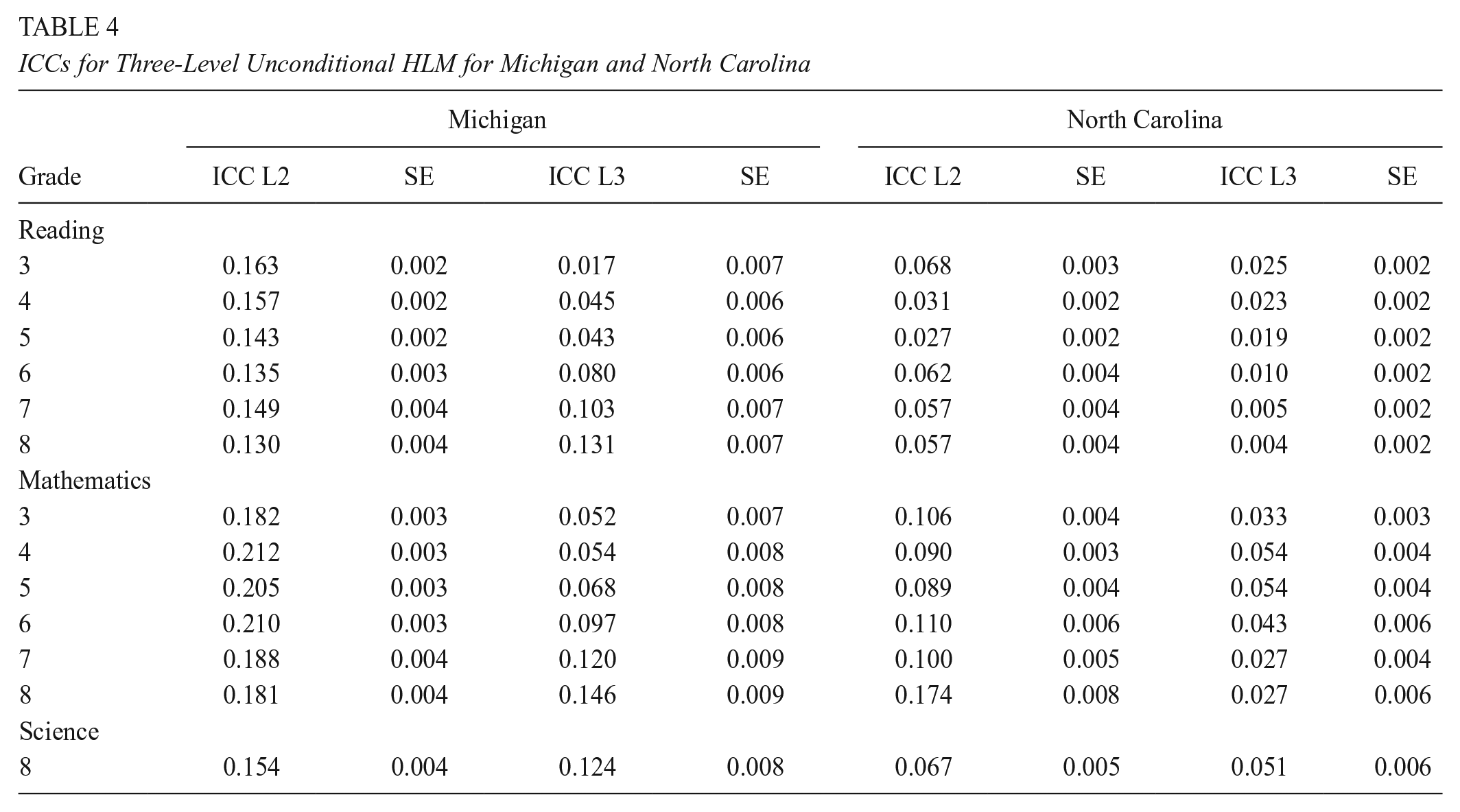
Tables 4 and 5 present the unconditional ICCs for the three-level models, with students nested in teachers nested in schools. These results reveal key patterns and differences in ICCs, including distinctions between elementary and middle school ICCs, variations across reading, mathematics, and science ICCs, differences between teacher and school ICCs, all while comparing across different states. To aid with the interpretation of the tables below, we will use the ICCs for Michigan grade 5 in reading as an example (see Table 4), where teacher-level ICC is .143 and school-level ICC is .043. This means that, in Michigan grade 5, 14.3% of the variance in student reading test scores is between teachers within schools, and 4.3% is between schools.

Table 4

ICCs for Three-Level Unconditional HLM for Michigan and North Carolina

Grade	Michigan				North Carolina
Grade	ICC L2	SE	ICC L3	SE	ICC L2	SE	ICC L3	SE
Reading
3	0.163	0.002	0.017	0.007	0.068	0.003	0.025	0.002
4	0.157	0.002	0.045	0.006	0.031	0.002	0.023	0.002
5	0.143	0.002	0.043	0.006	0.027	0.002	0.019	0.002
6	0.135	0.003	0.080	0.006	0.062	0.004	0.010	0.002
7	0.149	0.004	0.103	0.007	0.057	0.004	0.005	0.002
8	0.130	0.004	0.131	0.007	0.057	0.004	0.004	0.002
Mathematics
3	0.182	0.003	0.052	0.007	0.106	0.004	0.033	0.003
4	0.212	0.003	0.054	0.008	0.090	0.003	0.054	0.004
5	0.205	0.003	0.068	0.008	0.089	0.004	0.054	0.004
6	0.210	0.003	0.097	0.008	0.110	0.006	0.043	0.006
7	0.188	0.004	0.120	0.009	0.100	0.005	0.027	0.004
8	0.181	0.004	0.146	0.009	0.174	0.008	0.027	0.006
Science
8	0.154	0.004	0.124	0.008	0.067	0.005	0.051	0.006

Table 5

ICCs for Three-Level Unconditional HLM for Kentucky and Maryland

Grade	Kentucky				Maryland
Grade	ICC L2	SE	ICC L3	SE	ICC L2	SE	ICC L3	SE
Reading
3	0.054	0.004	0.113	0.007	0.121	0.005	0.196	0.010
4	0.061	0.004	0.096	0.007	0.167	0.006	0.185	0.010
5	0.082	0.005	0.088	0.007	0.146	0.006	0.205	0.011
6	0.214	0.011	0.079	0.012	0.278	0.013	0.170	0.018
7	0.300	0.014	0.070	0.013	0.301	0.013	0.157	0.018
8	0.317	0.014	0.091	0.015	0.284	0.014	0.163	0.018
Mathematics
3	0.071	0.004	0.128	0.008	0.177	0.006	0.191	0.011
4	0.075	0.005	0.134	0.009	0.236	0.008	0.177	0.012
5	0.096	0.006	0.125	0.009	0.297	0.009	0.170	0.012
6	0.192	0.010	0.124	0.014	0.398	0.016	0.176	0.020
7	0.234	0.012	0.078	0.012	0.391	0.015	0.186	0.020
8	0.248	0.012	0.130	0.016	0.352	0.015	0.186	0.020
Science
7	0.134	0.011	0.109	0.015
8					0.160	0.009	0.264	0.019

In terms of patterns, Table 4 reveals a similar pattern across Michigan and North Carolina, where the teacher-level variance is larger than the school-level variance. For example, in Michigan, in grade 3, about 2% of the variance in reading test scores is between schools, 16% is between teachers within schools, and the remaining 82% is between students within teachers. This means that there is more variability in math achievement between teachers within a school than between schools. Kentucky and Maryland in Table 5, however, show a different pattern, where for elementary school grades, the teacher-level variance is smaller than the school-level variance, meaning there is more variability between schools in Kentucky and Maryland than within schools. While in Kentucky this pattern is visible in both reading and mathematics, in Maryland, however, the school-level variance is larger than the teacher-level variance in reading only, and in third-grade math. In general, North Carolina had the smallest estimates in both teacher and school level across the grades and subjects, compared to Michigan, Kentucky, and Maryland. Finally, as seen in Tables 4 and 5, the results showed larger teacher- and school-level ICCs in mathematics, compared to reading and science.

Percentage of Variance Explained

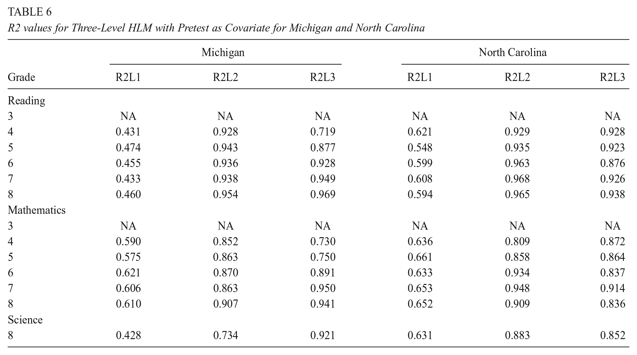
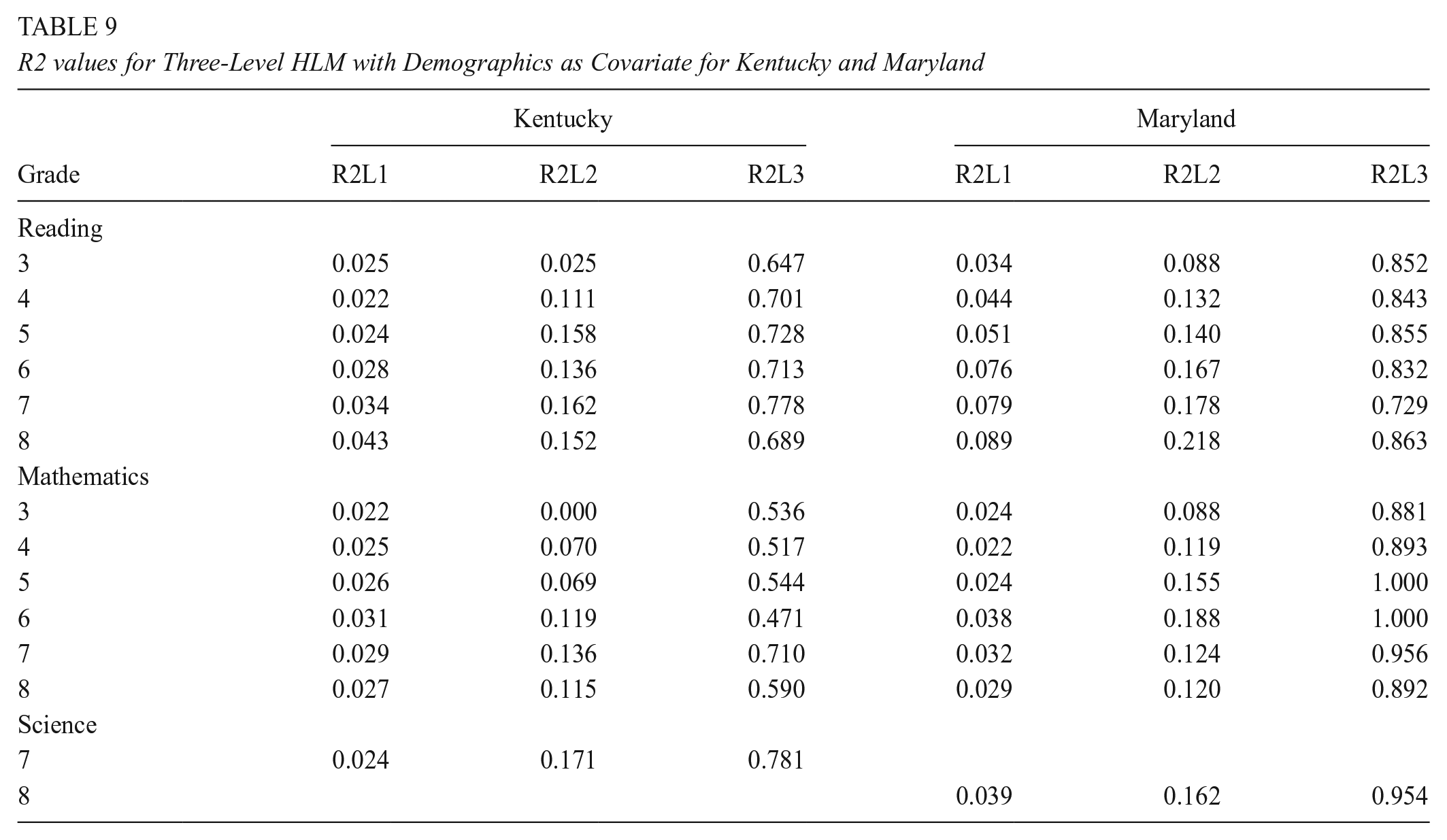
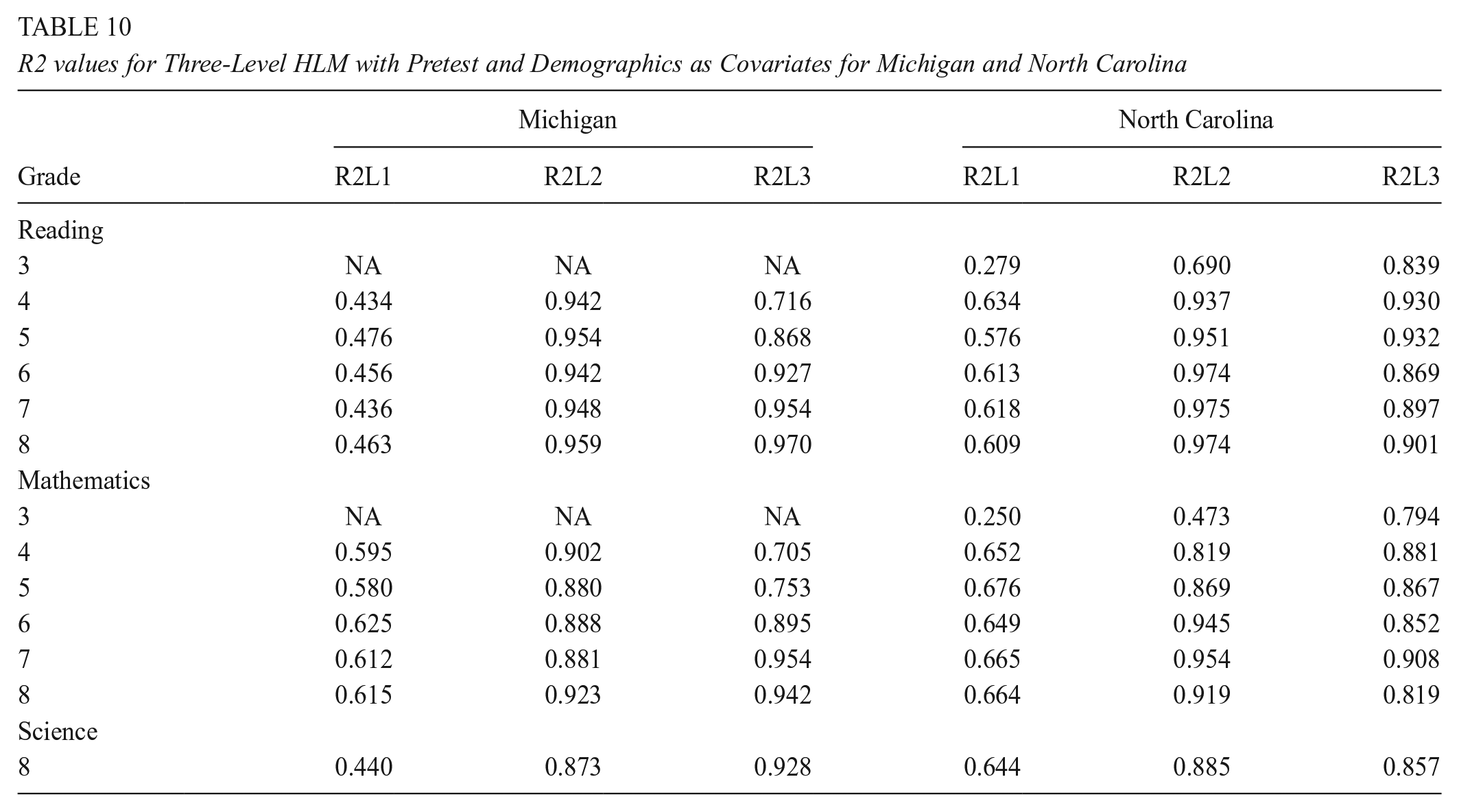
In this section, we present the results for the three-level model where student-level pretests and demographics were examined as covariates. First, in Tables 6 and 7, we present the results where the student-level pretest was examined as a covariate, including student-level individual scores in reading, mathematics, and science, and teacher- and school-level averages of the student-level. These results explain the variation at the student-, teacher- and school level. Note that the only exception to this is for grade 3, which is the first year that students are tested, thus there was no pretest data available. In Tables 8 and 9, we present the results where demographic variables were examined as covariates, including race, gender, and lunch status. Lastly, in Tables 10 and 11, we present the results where both student-level pretest and demographics were examined as covariates.

Table 6

R2 values for Three-Level HLM with Pretest as Covariate for Michigan and North Carolina

Grade	Michigan			North Carolina
Grade	R2L1	R2L2	R2L3	R2L1	R2L2	R2L3
Reading
3	NA	NA	NA	NA	NA	NA
4	0.431	0.928	0.719	0.621	0.929	0.928
5	0.474	0.943	0.877	0.548	0.935	0.923
6	0.455	0.936	0.928	0.599	0.963	0.876
7	0.433	0.938	0.949	0.608	0.968	0.926
8	0.460	0.954	0.969	0.594	0.965	0.938
Mathematics
3	NA	NA	NA	NA	NA	NA
4	0.590	0.852	0.730	0.636	0.809	0.872
5	0.575	0.863	0.750	0.661	0.858	0.864
6	0.621	0.870	0.891	0.633	0.934	0.837
7	0.606	0.863	0.950	0.653	0.948	0.914
8	0.610	0.907	0.941	0.652	0.909	0.836
Science
8	0.428	0.734	0.921	0.631	0.883	0.852

Table 7

R2 values for Three-Level HLM with Pretest as Covariate for Kentucky and Maryland

Grade	Kentucky			Maryland
Grade	R2L1	R2L2	R2L3	R2L1	R2L2	R2L3
Reading
3	NA	NA	NA	NA	NA	NA
4	0.507	0.835	0.852	0.634	0.907	0.897
5	0.523	0.934	0.820	0.669	0.908	0.928
6	0.490	0.961	0.691	0.642	0.976	0.847
7	0.511	0.979	0.814	0.663	0.977	0.927
8	0.496	0.987	0.854	0.668	0.973	0.940
Mathematics
3	NA	NA	NA	NA	NA	NA
4	0.579	0.740	0.663	0.680	0.930	0.886
5	0.612	0.845	0.649	0.648	0.948	0.899
6	0.571	0.925	0.494	0.618	0.975	0.907
7	0.587	0.956	0.665	0.615	0.961	0.981
8	0.562	0.957	0.611	0.583	0.911	0.971
Science
7	0.425	0.963	0.586
8				0.571	0.962	0.910

Table 8

R2 values for Three-Level HLM with Demographics as Covariate for Michigan and North Carolina

Grade	Michigan			North Carolina
Grade	R2L1	R2L2	R2L3	R2L1	R2L2	R2L3
Reading
3	0.022	0.785	0.075	0.279	0.690	0.839
4	0.019	0.830	0.160	0.634	0.937	0.930
5	0.019	0.850	0.158	0.576	0.951	0.932
6	0.015	0.844	0.233	0.613	0.974	0.869
7	0.017	0.855	0.197	0.618	0.975	0.897
8	0.016	0.876	0.159	0.609	0.974	0.901
Mathematics
3	0.025	0.738	0.044	0.250	0.473	0.794
4	0.033	0.808	0.075	0.652	0.819	0.881
5	0.028	0.739	0.121	0.676	0.869	0.867
6	0.029	0.734	0.143	0.649	0.945	0.852
7	0.029	0.753	0.144	0.665	0.954	0.908
8	0.031	0.796	0.132	0.664	0.919	0.819
Science
8	0.026	0.874	0.160	0.644	0.885	0.857

Table 9

R2 values for Three-Level HLM with Demographics as Covariate for Kentucky and Maryland

Grade	Kentucky			Maryland
Grade	R2L1	R2L2	R2L3	R2L1	R2L2	R2L3
Reading
3	0.025	0.025	0.647	0.034	0.088	0.852
4	0.022	0.111	0.701	0.044	0.132	0.843
5	0.024	0.158	0.728	0.051	0.140	0.855
6	0.028	0.136	0.713	0.076	0.167	0.832
7	0.034	0.162	0.778	0.079	0.178	0.729
8	0.043	0.152	0.689	0.089	0.218	0.863
Mathematics
3	0.022	0.000	0.536	0.024	0.088	0.881
4	0.025	0.070	0.517	0.022	0.119	0.893
5	0.026	0.069	0.544	0.024	0.155	1.000
6	0.031	0.119	0.471	0.038	0.188	1.000
7	0.029	0.136	0.710	0.032	0.124	0.956
8	0.027	0.115	0.590	0.029	0.120	0.892
Science
7	0.024	0.171	0.781
8				0.039	0.162	0.954

Table 10

R2 values for Three-Level HLM with Pretest and Demographics as Covariates for Michigan and North Carolina

Grade	Michigan			North Carolina
Grade	R2L1	R2L2	R2L3	R2L1	R2L2	R2L3
Reading
3	NA	NA	NA	0.279	0.690	0.839
4	0.434	0.942	0.716	0.634	0.937	0.930
5	0.476	0.954	0.868	0.576	0.951	0.932
6	0.456	0.942	0.927	0.613	0.974	0.869
7	0.436	0.948	0.954	0.618	0.975	0.897
8	0.463	0.959	0.970	0.609	0.974	0.901
Mathematics
3	NA	NA	NA	0.250	0.473	0.794
4	0.595	0.902	0.705	0.652	0.819	0.881
5	0.580	0.880	0.753	0.676	0.869	0.867
6	0.625	0.888	0.895	0.649	0.945	0.852
7	0.612	0.881	0.954	0.665	0.954	0.908
8	0.615	0.923	0.942	0.664	0.919	0.819
Science
8	0.440	0.873	0.928	0.644	0.885	0.857

Table 11

R2 values for Three-Level HLM with Pretest and Demographics as Covariates for Kentucky and Maryland

Grade	Kentucky			Maryland
Grade	R2L1	R2L2	R2L3	R2L1	R2L2	R2L3
Reading
3	NA	NA	NA	NA	NA	NA
4	0.507	0.837	0.865	0.638	0.908	0.907
5	0.523	0.935	0.833	0.674	0.908	0.936
6	0.490	0.963	0.731	0.649	0.976	0.864
7	0.511	0.980	0.842	0.668	0.977	0.933
8	0.497	0.988	0.850	0.673	0.973	0.953
Mathematics
3	NA	NA	NA	NA	NA	NA
4	0.579	0.747	0.681	0.683	0.930	0.914
5	0.612	0.846	0.664	0.650	0.949	0.904
6	0.571	0.927	0.563	0.624	0.975	0.929
7	0.587	0.956	0.717	0.618	0.962	0.987
8	0.562	0.959	0.652	0.585	0.912	0.980
Science
7	0.426	0.962	0.663
8				0.570	0.960	0.910

Unlike our findings for ICCs, a similar pattern emerged across all four states where the percentage of variance explained at the teacher level by pretest was larger than the percentage of variance explained by pretest at the school level, and the percentage explained at student level was smaller than the percentage explained at teacher- and school-level. Moreover, for grade 8 in Michigan, for example, the percentage of variance explained by reading pretest at both teacher and school level is higher than for the mathematics or science pretest. The results showed that across all states, the reading pretest explains more variability than either the mathematics or science pretest.

Tables 8 and 9 where demographic variables were included as covariates in the model, show that, overall, the patterns between elementary and middle-school grades, were similar in Michigan, Kentucky, and Maryland, where demographic variables explained more of the variance at the teacher level. In North Carolina middle schools, however, the differences in student test scores in reading and mathematics are more strongly related to the differences between teachers than they are in elementary schools. This might imply that teacher demographics might affect student outcomes more in middle school compared to elementary school.

Finally, including both student pretest and demographics in the model helps explain slightly more variance in student outcomes. Our results in Tables 10 and 11 showed that for each of the subjects, and at each level, the percentage of the variance explained by our combined set of variables increased. For example, for Michigan grade 4, at the teacher level, while the pretest only explained 93% of the variance, and demographics explained 83% of the variance, both combined explained about 94% of the variance in student reading outcomes. However, the difference in percentage explained between the first model where only the pretest was included as a covariate, and the third model where both the pretest and demographic were included as covariates was negligible, with an average of .007 units difference (not including the teacher level R² value in Michigan, where the difference was .14) so it remains at the researchers’ discretion on which is the most appropriate model to use its estimates.

Applications

Power Analyses for CRTs and MSCRTs

This paper demonstrates how applied researchers could use the design parameters from the tables presented in this study to conduct a power analysis. In this section, we provide examples of how the researchers could use those parameters in different scenarios. In Table 12, we show the parameters necessary in conducting an a priori power analysis for the main effect of treatment for a three-level CRT with students nested in teachers nested in schools and random assignment at the school level, and for an MSCRT with students nested within teachers nested within schools, and random assignment at the teacher level. Note that the same design parameters are necessary for the power analysis for the three-level CRTs and MSCRT, except for an additional parameter for the MSCRT with random effects. In that case, researchers need to estimate the Level 3 treatment effect heterogeneity, or the variance in the treatment effect across Level 3 units, standardized by the Level 3 outcome variation (marked with the Greek letter ω). We assume random effects in this example.

Table 12

Necessary Parameters for Power Analysis for Three-Level CRT and MSCRT

Necessary Parameters
Alpha level (α) – Probability of Type I error
Two-tailed or One-tailed Test Specification
Power (1-β) – Statistical power (1-probability of a Type II error)
g – Number of Level 3 covariates
P – Proportion of Level 3 units randomized to treatment
ICC_L2 – proportion of variance between teachers within schools (Level 2 units)ICC_L3 – proportion of variance between schools (Level 3 units)
R²_L3 – proportion of school-level variance explained by covariatesR²_L2 – proportion of teacher-level variance explained by covariatesR²_L1 – proportion of student-level variance explained by covariates
K – number of schools (sample size, number of Level 3 units)J – average number of teachers per school (average sample size for Level 2)I – average number of students per school (average sample size for Level 1)
* ω₃ – Level 3 treatment effect heterogeneity: variance in treatment effect across Level 3 units, standardized by Level 3 outcome variation.

This parameter is relevant only for MSCRT with random effects.

When conducting power analyses for CRTs and MSCRTs, researchers often approach it from the perspective of determining the minimum detectable effect size (MDES), which represents the smallest true mean program effect or effect size that a study design can detect at a specific level of statistical significance, which is commonly .05 for two-tailed tests, and a specific level of statistical power, which is typically 80% (Bloom, 2005; Bloom & Spybrook, 2017). For three-level CRTs with students nested within teachers nested within schools, the number of schools is the most influential in determining the MDES. In MSCRTs, the number of teachers may play a more important role, particularly when the treatment effect can vary randomly across sites as in the case of an MSCRT with random effects (Bloom & Spybrook, 2017).

The design parameters presented in Tables 4 through 12 can serve in planning reading, mathematics, and science impact studies that use a CRT or MSCRT. We created two research scenarios where these design parameters were used. First, we considered a three-level CRT, with students nested in teachers nested in schools, and randomization at the school level. Second, since the main contribution of this study was around the teacher level, we also considered a three-level MSCRT with teachers randomly assigned to a treatment condition within schools and students nested within teachers. In both scenarios, the power was set to 80%, the significance level at .05, and they had balanced designs with 50% of the schools in CRT and teachers in MSCRT receiving the treatment, and the other 50% serving as a comparison group. All of the calculations were done using PowerUp! (Dong & Maynard, 2013; Dong et al., 2017).

Scenario 1: MDES for Main Effects (3-level CRT)

In this first hypothesized scenario, suppose a team of researchers is designing a study to test the efficacy of a new mathematics curriculum for fourth graders. The researchers will implement the study in Kentucky, where there are approximately 40 participating schools, 4 teachers per school, and 25 students per teacher. The team conducts a power analysis to determine the MDES (Bloom, 1995).

To calculate the MDES, relevant estimates of the ICC will be used from Table 5 where the teacher-level ICC was estimated at .075 in Kentucky and the school-level ICC was estimated at .134. For estimates of R², the researchers want to use only the student pretest (see Table 7) as they are aware that traditionally, demographic covariates explain very little variance (Bloom et al., 2007; Hedges & Hedberg, 2013; Spybrook et al., 2016a; Westine et al., 2013). So, given the provided number of clusters, sample size, and ICC and R² values, the researchers were able to detect an MDES of .210 in Kentucky. The detected effect size is comparable to the range Hill et al. (2008) suggested for educational intervention, which was .20 to .30.

Scenario 2: MDES for Main Effects (3-level MSCRT)

In this second scenario, suppose the same research team designed the study so that only the teachers receiving the treatment are provided with a tablet to prepare their notes and implement the respective math curriculum for grade 4. Due to this intervention’s nature, it is reasonable to conduct an MSCRT with treatment assigned at the teacher level. Like in the previous scenario, the researchers will conduct their study in Kentucky. In this scenario, each participating school is considering assigning teachers to the new curriculum or the business-as-usual condition. As in the previous scenario, there are approximately 40 participating schools, 4 teachers per school, and 25 students per teacher. To determine the MDES, the researchers decided to conduct a power analysis using the MDES calculator for a three-level random effects blocked cluster randomized assignment design, with assignment at level 2.

Also, here, estimates of ICC will be used from Table 5 and estimates or R² values from Table 7 where the model included student pretest as covariate. Consistent with Weiss et al. (2017) study of 16 MSCRTs in education, the Level 3 treatment effect heterogeneity was set at .05 which is operationalized as equivalent to 5 percent of the variance of means at level 3. Power calculations showed the researchers would be able to detect an MDES value of .107.

Comparison of Power Analysis with and without the Teacher Level

For comparison purposes, we ran power analysis using the same assumptions as in the first scenario demonstrated above where we computed the MDES for Main Effects (3-level CRT). However, instead of using the ICC values derived empirically in this study, we used the rule of thumb, where we computed two-level models with students nested in schools, and then we decomposed the school-level ICC from the two-level model, such that two-thirds of the original school-level ICC estimate remained at the school level, and one-third of the original school-level ICC estimate was moved to the teacher level.

In line with the first scenario, for a math curriculum study for fourth graders in Kentucky, we assumed 40 participating schools, 4 teachers per school, and 25 students per teacher. From Table 2 in Appendix A, we decomposed the respective school-level ICC (.12). This led to a teacher-level ICC of .04 and a school-level ICC of .08 (note that using empirical estimates, the teacher-level ICC was .075 and the school-level ICC was .134). We used the same R² values as in the first scenario with only the student pretest (see Table 7). Given the provided number of clusters, sample size, and ICC and R² values, using the rule of thumb, the results indicated that the researcher would be able to detect an MDES of .16, which is smaller than what the MDES value suggested by using empirical ICCs (.21). This demonstration shows that using the rule of thumb ICCs might be misleading for researchers, and in this case, potentially underestimating the MDES they can detect given their sample size.

Implication of Power Analysis for Recruitment Processes

While this paper does not provide all possible design parameter values that any current or future evaluation team may need, this paper does importantly show that evaluators must work with partner schools, districts, and states to obtain information on how student achievement varies by teachers within schools. Such an investigation would not require student data per se, but if teacher-level means, counts, and standard deviations were available from districts and/or potential schools, values for teacher- and school-level ICCs could be computed using variance component formulas based on analysis of variance tables (see, e.g., Searle et al., 2009).

Discussion

This study highlights the importance of considering all levels of the learning environment’s landscape. Students, teachers, and schools all play a role in shaping the environment, which can lead to differences in student achievement. Therefore, we examined the role teachers play in student achievement and the learning environment by calculating empirical estimates of design parameters for the teacher level. We decomposed the variance in mathematics, reading, and science test scores to the student, teacher, and school levels and examined how it varied across states. Lastly, we provided practical applications demonstrating how to calculate power for three-level CRTs and MSCRTs.

The empirical estimates provided in this study regarding the variance in mathematics, reading, and science test scores between teachers and schools showed different patterns across states. On average, North Carolina had the lowest between-teacher variance and between-school variance compared to other states. Furthermore, across all states, there were differences in the variance between teachers and between schools across grades, where middle school grades had higher values of between-teacher variance compared to elementary school grades. One possible explanation for this trend may be the sorting of students across classes within schools that occurs in middle school based on their abilities. For example, schools offer more advanced course pathways in mathematics and readings only for students who are high performers, and thus we might notice such differences in middle school ICCs. However, for this explanation to be conclusive, we would need to conduct further analysis.

This paper showed notable differences in findings across states in terms of ICC values and the relative size of teacher and school ICCs. Some of the reasons for observing such differences across states might be related to states’ population heterogeneity (variations in demographics and socio-economic status); district and state contextual factors and policies regarding student-teacher assignment and organizational influence on teaching practices, economic conditions, and environmental conditions, which individually or in combination may influence the impact of teachers on student achievement. These potential sources of variability across states are important to be explored further in future studies and supplement the analysis with qualitative research methods to better understand contextual factors. Thus, as a major takeaway, this paper shows that there are important contextual factors that must be considered when planning a study in a single state.

As expected, the empirical estimates of the percentage of variance explained by demographics and pretests for all three subjects showed that student pretests explained a higher portion of the variance in student achievement compared to demographics. A similar pattern we noticed across the states was that the percentage of variance explained by teacher- and school-level reading pretests appeared to be higher than for the mathematics pretest, which may indicate that reading relative achievement is more stable from grade to grade than mathematics. Furthermore, teacher-level had the highest explanatory power in middle school grades, compared to the student level or the school level.

Most of the studies in literature examined the domains of reading and mathematics. Empirical evidence suggests that design parameters for one domain may not be the same as another (e.g., Westine et al., 2013). That is, the contribution of teachers and schools plays out differently for science achievement than for reading achievement, as it was suggested by our findings. Hence, in this study, we deemed it was important to consider science in addition to reading and mathematics and analyze the variance the teacher level contributes to each of these subjects. We included the three subjects to help researchers planning CRTs to have subject and grade-specific parameter estimates, as opposed to borrowing estimation from other subjects, which will reduce the precision in power estimations. Given that our study included results from four states only, we recommend that researchers consider state-specific variables that may influence ICC values, such as demographics, regional policies, or socio-economic factors. This ensures that the results are contextualized appropriately. Furthermore, we also recommend small pilot studies from a specific state using similar approaches to those we covered in this paper, to help researchers compare design parameters across different states, as well as contribute to the precision of the parameters when computing statistical power.

While this study excluded students with cognitive-related IEPs, the results of our studies are not likely to negatively impact study planning if such students were to be included. It is likely that including these students would result in slightly smaller ICC values, as students with cognitive-related IEPs are likely to have lower scores on state exams, which given the limited members of this population in the total student population is more likely to add more to the residual variance than any clusters’ variance. This assumes that students with cognitive-related IEPs are integrated in general education classrooms. For example, if we examine earlier results which are stored in online-tables such as Online intraclass correlation database (Institute for Policy Research, n.d), we see that the school ICC for all fifth grade Massachusetts students for math achievement is about .31 (SE = .06), whereas the school ICC for the same grade and subject, but for students with cognitive-related IEPs, is .26 (SE = .02), which is smaller. However, this difference of .05 has a variance of approximately .06 if we assume these are independent estimates or .04 if we assume the sampling correlation of .99, neither of which results in a statistically significant difference.

While studies with teacher ICC values are limited to a few states, our results have indicated that often a majority of the variance associated with the clusters in which students are nested relate to teachers rather than schools. Since we have shown that “rules of thumb” from other scholars did not apply to our limited set of states, we are hesitant to provide another rule of thumb with likely limited utility. We encourage researchers to use this paper in their discussions with the districts and states they work with to encourage sharing data or running analyses on student achievement, with teacher and other applicable random effects, so that appropriate ICC values can be used in study planning. Short of this, a conservative approach would be to use available school ICCs as both the school and teacher ICC and not to split the school ICC into composite school and teacher values. This will result in a much larger MDES or required sample values, of course, but will also avoid underpowering studies.

Limitations and Future Directions

This paper represents an important contribution for researchers interested in planning studies to evaluate the effectiveness of different educational interventions. The availability of design parameters for the teacher level will allow the researchers to conduct more precise power analyses for studies that include the teacher level. While this work is important in its own right, it also lays the foundation for additional extensions that can take place to help the field grow.

One extension of this work might be to further explore ICCs of states by focusing on state demographics, including the locale of their school and districts, the school sizes, and the socio-economic status of the school. Such work is necessary to provide researchers with more specific design parameters so they can use those for their own research context similar to those presented in this potential study.

Second, the current study is focused on grades 3 to 8, thus excluding high school grades. It is important to expand this work to also include the high school grades, and then compare the ICCs between different grades, such as elementary, middle, and high school grades. Such a study is important, especially for the researchers that focus on intervention at the high school level.

Third, the current results from this paper are useful for the main effects. There is more work that needs to be done to also understand and evaluate teacher moderator effects as they play a very important role in delivering educational interventions. The inclusion of the teacher level in empirical estimates of ICCs will allow researchers to conduct power analyses to detect teacher-level moderator effects, which is an important next step in expanding the existing work.

Lastly, while the quantitative methods of research can allow us as researchers to understand variability in student achievement and statistically explain it at different levels of nesting, as shown in this study, differences exist between states. Therefore, it is important in the future to take these results and conduct a study using qualitative methods of inquiry, such as grounded theory (Charmaz, 2006; Corbin & Strauss, 2015), by conducting interviews with representative of states’ educational departments and tap into their experiences, stories, historical development of the education policies, and understanding of their respective states context (Mulolli & Gothberg, 2023). This way, we will be able to have a clearer picture of the reasons we are witnessing such variability in student achievement at different levels of nesting across states.

Some of the limitations of this study include the following: given the use of convenience sampling of our states, the results of this study represent four states in total. In the future, it is important to run similar analyses in other states and compare the findings. In this study, we excluded students with cognitive disabilities. While we provide our reasons for making this decision in this paper, it would be important to add them back to the analytical sample in the future.

Footnotes

Appendix A

Acknowledgements

This research was supported by the Maryland Longitudinal Data System (MLDS) Center. We are grateful for the assistance provided by the MLDS Center. All opinions are the authors’ and do not represent the opinion of the MLDS Center or any of their partner agencies.

This research result used data structured and maintained by the MERI-Michigan Education Data Center (MEDC). MEDC data is modified for analysis purposes using rules governed by

MEDC and are not identical to those data collected and maintained by the Michigan Department of Education (MDE) and/or Michigan’s Center for Educational Performance and Information (CEPI). Results, information and opinions solely represent the analysis, information and opinions of the author(s) and are not endorsed by, or reflect the views or positions of, grantors, MDE and CEPI or any employee thereof.

The information and data presented in this publication were provided by the Kentucky Department of Education (KDE). The opinions, findings, conclusions, and recommendations expressed in this publication are those of the authors and do not necessarily reflect the views or policies of the Kentucky Department of Education.

The data used in this publication were provided by the North Carolina Department of Public Instruction (NCDPI). The opinions, findings, conclusions, and recommendations expressed in this publication are those of the authors and do not necessarily reflect the views or policies of the North Carolina Department of Public Instruction.

Funding

The author(s) disclosed receipt of the following financial support for the research, authorship, and/or publication of this article: This work was funded by the National Science Foundation, Award 2000388.

ORCID iDs

Dea Mulolli

E.C. Hedberg

Megan Bogia

Jessaca Spybrook

Isaac M. Opper

Open Practices Statement

We have deposited the materials for this research to ICPSR to promote transparency and facilitate further research. The process on how to obtain student-level data from states is outlined and the R scripts to conduct analysis are included in our deposit which is publicly accessible for review and reuse, adhering to open science principles. You can access the deposit here: .

Authors

DEA MULOLLI is a research scientist at Human Resources Research Organization (HumRRO), Alexandria, VA; email: dmulolli@humrro.org. Her research is focused on power analysis, student achievement, and improving evaluation of educational research.

ERIC (E. C.) HEDBERG is a principal research associate (Education Studies Practice) at Westat, Rockville, MD; email: erichedberg@westat.com. His research areas include estimating design parameters for planning impact evaluations and creating tools to evaluate the sensitivity of various random and non-random designs.

MEGAN BOGIA is an Associate Director for Academic Programs and Strategic Initiative at Fordham University Center for Ethics Education, New York City, NY. Email: mbogia@fordham.edu. Her research combines empirical and normative analyses to examine problems of postsecondary policy ethics.

JESSACA K. SPYBROOK is a former professor in the Evaluation, Measurement, and Research Program at Western Michigan University and is currently serving as managing director at American Institutes for Research (AIR), Arlington, VA. Email: jspybrook@air.org. Her research interests are in the design and analysis of large-scale impact studies.

TIFFANY BERGLUND is a quantitative analyst at the RAND Corporation, Santa Monica, CA. Email: ttsai@rand.org. Her research addresses college access, school improvement, and military recruiting resource allocation.

FATIH UNLU is a senior manager at Amazon, Santa Monica, CA. Email: fatihunlu@gmail.com. His research interests include evaluations of education and workforce development programs and interventions.

ISAAC M. OPPER is a senior economist at the RAND Corporation and a professor of public policy at the Pardee RAND Graduate School, Santa Monica, CA. Email: isaac_opper@rand.org. His work has studied teacher personnel policies and the measurement of teacher effectiveness, peer effects in the education setting, and the impact of natural disasters on human capital accumulation.

References

Bloom

H. S.

(1995). Minimum detectable effects: A simple way to report the statistical power of experimental designs. Evaluation Review, 19(5), 547–556. https://doi.org/10.1177/0193841x9501900504

Bloom

H. S.

(2005). Randomizing group to evaluate place-based programs. In Bloom

H. S.

(Ed.), Learning more from social experiments: Evolving analytic approaches (pp. 115–172). Russel Sage.

Bloom

H. S.

Spybrook

(2017). Assessing the precision of multisite trials for estimating the parameters of a cross-site population distribution of program effects. Journal of Research on Educational Effectiveness, 10(4), 877–902. https://doi.org/10.1080/19345747.2016.1271069

Bloom

H. S.

Richburg-Hayes

Rebeck-Black

(2007). Using covariates to improve precision for studies that randomize schools to evaluate educational interventions. Educational Evaluation and Policy Analysis, 29(1), 30–59. https://doi.org/10.3102/0162373707299550

Brandon

P. R.

Harrison

G. M.

Lawton

B. E.

(2013). SAS code for calculating intraclass correlation coefficients and effect size benchmarks for site-randomized education experiments. American Journal of Evaluation, 34(1), 85–90. https://doi.org/10.1177/1098214012466453

Bulger

McCormick

Pitcan

(2017). The legacy of inBloom. Data&Society. https://datasociety.net/pubs/ecl/InBloom_feb_2017.pdf

Chan

Hedges

L. V.

Hedberg

E. C.

(2022). The effects of downstream clustering in longitudinal studies. Journal of Experimental Education, 90(3), 731–759. https://doi.org/10.1080/00220973.2020.1783501

Charmaz

(2006). Constructing grounded theory: A practical guide through qualitative analysis. Sage.

Cohen

(1988). Statistical power analysis for the behavioral sciences (2nd ed.). Lawrence Elbraum Associates, Publishers.

10.

Corbin

Strauss

(2015). Basics of qualitative research: Techniques and procedures for developing grounded theory (4th ed.). Sage.

11.

Dong

Maynard

R. A.

(2013). PowerUp!: A tool for calculating minimum detectable effect sizes and sample size requirements for experimental and quasi-experimental designs. Journal of Research on Educational Effectiveness, 6(1), 24–67. https://doi.org/10.1080/19345747.2012.673143

12.

Dong

Reinke

W. M.

Herman

K. C.

Bradshaw

C. P.

Murray

D. W.

(2016). Meaningful effect sizes, intraclass correlations, and proportions of variance explained by covariates for planning two- and three-level cluster randomized trials of social and behavioral outcomes. Evaluation Review, 40(4), 334–377. https://doi.org/10.1177/0193841X16671283

13.

Dong

Kelcey

Spybrook

Maynard

R. A.

(2017). PowerUp!-Moderator: A tool for calculating statistical power and minimum detectable effect size of the moderator effects in cluster randomized trials (Version 1.08) [Computer software]. http://www.causalevaluation.org/

14.

Glander

(2016). Documentation to the NCES Common Core of Data public elementary/secondary school universe survey: School year 2013–14. Provisional Version 2a (NCES 2015-150rev). National Center for Education Statistics.

15.

Hedberg

E. C.

(2016). Academic and behavioral design parameters for cluster randomized trials in kindergarten: An analysis of the early childhood longitudinal study 2011 kindergarten cohort (ECLS-K 2011). Evaluation Review, 40(4), 279–313. https://doi.org/10.1177/0193841X16655657

16.

Hedges

L. V.

Hedberg

E. C.

(2007). Intraclass correlation values for planning group-randomized trials in education. Educational Evaluation and Policy Analysis, 29(1), 60–87. https://doi.org/10.3102/0162373707299706

17.

Hedges

L. V.

Hedberg

E. C.

Kuyper

A. M.

(2012). The variance of intraclass correlations in three-and four-level models. Educational and Psychological Measurement, 72(6), 893–909. https://doi.org/10.1177/0013164412445193

18.

Hedges

L. V.

Hedberg

E. C.

(2013). Power calculation using the online variance almanac (Web VA): A user’s guide. Center for Advancing Research and Communication in Science, Technology, Engineering and Mathematics (ARC). NORC at the University of Chicago, Chicago, IL. Retrieved from https://arc.uchicago.edu/reese/variance-almanac-academic-achievement

19.

Hill

C. J.

Bloom

H. S.

Rebeck-Black

Lipsey

M. W.

(2008). Empirical benchmarks for interpreting effect sizes in research. Child Development Perspectives, 2(3), 172–177. https://doi.org/10.1111/j.1750-8606.2008.00061.x

20.

Gabbin

C. P.

(2020). Teachers’ experiences implementing evidence-based interventions with fidelity for preschool-students with disabilities [Doctoral dissertation, Walden University]. Walden Dissertations and Doctoral Studies Collection at ScholarWorks.

21.

Institute for Policy Research. (n.d.). Online Intraclass correlation database. https://steppcenter.shinyapps.io/ICC_Database_Hedges_Hedberg/

22.

Jacob

Zhu

Bloom

H. S.

(2010). New empirical evidence for the design of group randomized trials in education. Journal of Research on Educational Effectiveness, 3(2), 157–198. https://doi.org/10.1080/19345741003592428

23.

Kelcey

Phelps

(2013). Considerations for designing group randomized trials of professional development with teacher knowledge outcomes. Educational Evaluation and Policy Analysis, 35(3), 370–390. https://doi.org/10.3102/0162373713482766

24.

Konstantopoulos

(2008a). How consistent are class size effects? Evaluation Review, 35(1), 71–92. https://doi.org/10.1177/0193841X11399847

25.

Konstantopoulos

(2008b). The power of the test for treatment effects in three-level cluster randomized designs. Journal of Research Effectiveness, 1(1), 66–88. https://doi.org/10.1080/19345740701692522

26.

Moerbeek

(2004). The consequence of ignoring a level of nesting in multilevel analysis. Multivariate Behavioral Research, 39(1), 129–149. https://doi.org/10.1207/s15327906mbr3901_5

27.

Mulolli

Gothberg

J. E.

(2023). How doctoral students with low GRE scores succeed: A grounded theory study. Qualitative Report, 28(1), 14–32. https://doi.org/10.46743/2160-3715/2023.5672

28.

National Center for Education Statistics (NCES), Institute of Education Sciences (IES), U.S. Department of Education. ElSi Table Generator: Kentucky > Total Enrollment 2018–2019. https://nces.ed.gov/ccd/elsi/tablegenerator.aspx

29.

National Center for Education Statistics (NCES), Institute of Education Sciences (IES), U.S. Department of Education. ElSi Table Generator: Maryland > Total Enrollment 2018–2019. https://nces.ed.gov/ccd/elsi/tablegenerator.aspx

30.

National Center for Education Statistics (NCES), Institute of Education Sciences (IES), U.S. Department of Education. ElSi Table Generator: Michigan > Total Enrollment 2013–2014. https://nces.ed.gov/ccd/elsi/tablegenerator.aspx

31.

National Center for Education Statistics (NCES), Institute of Education Sciences (IES), U.S. Department of Education. ElSi Table Generator: North Carolina > Total Enrollment 2018–2019. https://nces.ed.gov/ccd/elsi/tablegenerator.aspx

32.

Nye

Hedges

L. V.

Konstantopoulos

(2000). The effects of small classes on academic achievement: The results of the Tennessee class size experiment. American Educational Research Journal, 37(1), 123–151. https://doi.org/10.3102/00028312037001123

33.

Nye

Konstantopoulos

Hedges

L. V.

(2004). How large are teacher effects? Educational Evaluation and Policy Analysis, 26(3), 237–257. https://doi.org/10.3102/01623737026003237

34.

Phelps

Kelcey

Jones

Liu

(2016). Informing estimates of program effects for studies of mathematics professional development using teacher content knowledge outcomes. Evaluation Review, 40(5), 383–409. https://doi.org/10.1177/0193841X16665024

35.

Raudenbush

S. W.

Bryk

A. S.

(2002). Hierarchical linear models. Applications and data analysis methods (2nd ed.). Sage Publications.

36.

Searle

S. R.

Casella

McCulloch

C. E.

(2009). Variance components. John Wiley & Sons.

37.

Shen

Curran

F. C.

You

Splett

J. W.

Zhang

(2023). Intraclass correlations for evaluating the effects of teacher empowerment programs on student educational outcomes. Educational Evaluation and Policy Analysis, 45(1), 134–156. https://doi.org/10.3102/01623737221111400

38.

Spybrook

Kelcey

Dong

(2016b). Power for detecting treatment by moderator effects in two and three-level cluster randomized trials. Journal of Educational and Behavioral Statistics, 2(1), 1–15. https://doi.org/10.3102/1076998616655442

39.

Spybrook

Westine

C. D.

Taylor

J. A.

(2016a). Design parameters for impact research in science education: A multistate analysis. AERA Open, 2(1), 1–15. https://doi.org/10.1177/2332858415625975

40.

Stallasch

E. S.

Ludtke

Artelt

Brunner

(2021). Multilevel design parameters to plan cluster-randomized intervention studies on student achievement in elementary and secondary school. Journal of Research on Educational Effectiveness, 14(1), 172–206. https://doi.org/10.1080/19345747.2020.1823539

41.

Weiss

M. J.

Bloom

H. S.

Verbitsky-Savitz

Gupta

Vigil

A. E.

Cullinan

D. N.

(2017). How much do the effects of education and training programs vary across sites? Evidence from past multisite randomized trials. Journal of Research on Educational Effectiveness, 10(4), 843–876. https://doi.org/10.1080/19345747.2017.1300719

42.

Westine

C. D.

Spybrook

Taylor

J. A.

(2013). An empirical investigation of variance design parameters for planning cluster-randomized trials of science achievement. Evaluation Review, 37(6), 490–519. https://doi.org/10.1177/0193841X14531584

43.

Unlu

Fesler

Edmunds

Schwartz

Glennie

(2014, November). Design parameters for commonly used outcome measures in research on high schools and postsecondary institutions [Presentation]. Association for Public Policy Analysis and Management, Albuquerque, NM.

44.

Nichols

(2010). New estimates of design parameters for clustered randomization studies: Findings from North Carolina and Florida. Urban Institute, National Center for Analysis of Longitudinal Data in Education Research.

Improving the Design of Evaluations that Include Students,Teachers,and Schools: An Empirical Investigation of Key Design Parameters

Abstract

Keywords

Introduction

The Utility of Teacher Design Parameters

Study Purpose

Method

Sample and Data

Analysis

Models

Unconditional Three-Level Model

A Note about Cross-Classified Models

Conditional Model

Results

Intraclass Correlations

Percentage of Variance Explained

Applications

Power Analyses for CRTs and MSCRTs

Scenario 1: MDES for Main Effects (3-level CRT)

Scenario 2: MDES for Main Effects (3-level MSCRT)

Comparison of Power Analysis with and without the Teacher Level

Implication of Power Analysis for Recruitment Processes

Discussion

Limitations and Future Directions

Footnotes

Appendix A

Acknowledgements

Funding

ORCID iDs

Open Practices Statement

Authors

References