Sage Journals: Discover world-class research

Abstract

The Common Guidelines for Education Research and Development were created as a joint effort between the Institute of Education Science and the National Science Foundation in an effort to streamline education research and contribute to an accumulation of knowledge that will lead to improved student outcomes. One type of research that emerged in the guidelines is impact research. In order to achieve the level of rigor expected for an impact study, it is common that a research team will employ a cluster randomized trial (CRT). This article provides empirical estimates of design parameters necessary for planning adequately powered CRTs focused on science achievement. Examples of how to use these parameters to improve the design of science impact studies are discussed.

Keywords

program evaluation science education evaluation experimental design hierarchical linear modeling

In 2011, the Institute of Education Sciences (IES), the research branch of the U.S. Department of Education, and the National Science Foundation (NSF) came together to create a joint committee to “establish cross-agency guidelines for improving the quality, coherence, and pace of knowledge development in science, technology, engineering and mathematics (STEM) education” (IES & NSF, 2011, p. 4). Two years later, the Common Guidelines for Education Research and Development were released, hereafter referred to as simply the Guidelines. Overall, the ultimate goal of the Guidelines is to create a common set of expectations for studies that will help streamline education research and development and contribute to an accumulation of knowledge that will ultimately improve student outcomes (IES & NSF, 2011).

The Guidelines identify six types of research, including (a) foundational research, (b) early-stage or exploratory research, (c) design and development research, (d) efficacy research, (e) effectiveness research, and (f) scale-up research. These six types are combined into three categories of research: research aimed at contributing to core knowledge (types [a] and [b]), research aimed at developing solutions to improve learning (type [c]), and research aimed at contributing to evidence of impact (types [d], [e], and [f]). Each category of studies is critical to knowledge generation, from basic research to the development of interventions to testing the effectiveness of these interventions for improving student outcomes. However, the focus of this article is on the third category, impact research.

According to the Guidelines, the goal of impact research is to generate “reliable estimates of the ability of a fully-developed intervention or strategy to achieve its intended outcomes” (IES & NSF, 2011, p. 9). Stated differently, the goal is to identify “what works” or what interventions improve student outcomes. The three types of impact research differ in terms of “the conditions under which the intervention is implemented and the populations to which the findings generalize” (IES & NSF, 2011, p. 9). Efficacy research focuses on testing an intervention under ideal conditions, often in one population, and may include higher-than-normal levels of support from the program developers. Effectiveness research focuses on testing an intervention under typical conditions, often in a limited number of populations, and with normal levels of support from the program developers. Scale-up research focuses on testing an intervention across a broad array of contexts, in multiple populations, and “without substantial developer involvement in implementation or evaluation” (IES & NSF, 2011, p. 9). In short, these types of impact studies differ in their intent to generalize effects across populations, contexts, and levels of authenticity in the implementation conditions. Across all three types of impact studies, the most common designs are the randomized control trial (RCT) and the quasiexperimental design (QED).

In the past decade, we have seen an increase in the number of impact studies that utilize RCTs and QEDs across the field of education. For example, since 2002, IES has funded over 175 impact studies that employ RCTs (www.ies.gov). The majority of these studies focus on reading and mathematics interventions, with only a small percentage focused on science interventions. However, a recent systematic review by Slavin, Lake, Hanley, and Thurston (2014) provides evidence that there has been a shift in recent years toward more impact studies in science education. Slavin et al. found in their review of studies starting in 1980 that only 23 of the 332 identified studies met inclusion criteria for rigorous designs, which included strong QEDs and RCTs, and that most qualifying studies were published in 2006 or later. More specifically, one qualifying study was published in 2006, five in 2007, and 11 in 2009 or later, for a total of 17 of the 23 studies being published in 2006 or later and only six studies being published between 1980 and 2005.

The role of large-scale impact studies in science education research has generated a lot of attention in the past few years. In 2012, the Journal of Research in Science Teaching dedicated a special issue to the topic, raising awareness within the science education research community about the issues associated with large-scale impact studies and the importance of addressing these issues as more of these studies are conducted. The articles included in the special issue focused on challenges associated with implementing impact studies (Lee & Krajcik, 2012; Lynch, Pyke, & Grafton, 2012), limitations of these studies (Penuel & Fishman, 2012), and results from impact studies (Heller, Daehler, Wong, Shinohara, & Miratrix 2012; Plass et al. 2012). In 2013, Taylor, Kowalski, Wilson, Getty, and Carlson added to this dialogue by discussing the specific methodological trade-offs to conducting large-scale impact studies in science education. They pointed out the importance of balancing rigorous research designs with the interests and needs of the districts and schools to implement high-quality impact studies. As the field expands to include more impact studies of science interventions, it is important to be aware of these challenges and trade-offs in the design and implementation of these studies. Although design and implementation are both critical, in this article we focus on the design of impact studies.

In order for these impact studies to generate high-quality and rigorous evidence of the effectiveness of the intervention, the study must have a strong research design. According to the Guidelines, this means a research plan that provides detailed discussion of the following six components: (a) the study design, (b) outcomes of interest and size of impact that is important for each outcome, (c) setting and population of interest, (d) sample and statistical power associated with the sample and design, (e) plan for data collection, and (f) plan for analyses and reporting. All six of these components are crucial to planning a rigorous impact study. However, in this article we focus on the sample and statistical power associated with impact studies of science interventions.

As noted above, the most common designs in impact studies are RCTs and QEDs. Although the statistical power considerations for QEDs are the same as those of RCT, we frame our presentation from the perspective of designing RCTs as this preference is consistent with the Guidelines document, which in referring to researchers indicates that “generally and when feasible, they should use designs in which treatment and comparison groups are randomly assigned” (IES & NSF, 2011, p. 21). This preference is rooted in a specific threat to the internal validity of a QED—selection bias (Shadish, Cook, & Campbell, 2002). That is, QEDs are faced with the increased likelihood that the groups being compared will be more different on observed and unobserved variables than had the groups been formed randomly. Moreover, we focus on improving the a priori statistical power calculations for impact studies that utilize a specific type of RCT design, the cluster randomized trial (CRT) or, synonymously, the group randomized trial (GRT). In a CRT, entire clusters, such as schools, are assigned to a condition. Given the nested structure of schools, with students nested within teachers nested within schools, and the fact that educational programs and interventions are often delivered at the school level, CRTs are common in education impact studies (Spybrook & Raudenbush, 2009). The results from the Slavin et al. (2014) review also suggest CRTs are more common than RCTs that randomly assign individuals to groups for studies of science interventions. Of the seven studies in the review that are RCTs, all of them used clusters as the unit of random assignment and thus are categorized as CRTs.

Statistical Power for CRTs

The nested structure of the data in a CRT necessarily makes the a priori power analysis more complex. The power for a two-level CRT with randomization at the school level depends on the following: the alpha level, the number of students per school, the total number of schools, the effect size, the intraclass correlation (ICC), and the percentage of variance explained by the covariate(s) (R²). The ICC is the percentage of total variance in the outcome, science test scores, that is between schools. For example, if the ICC is 0.15, then 15% of the variance in science test scores is between schools and 85% of the variance in science test scores is within schools. Higher values of the ICC suggest more variance between schools, which leads to a need for a larger number of schools in order to be able to detect the effect if it is present. For example, holding all other parameters constant, if 25% of the variance in science test scores is between schools, more schools will be required to detect the same size effect than if only 15% of the variance is between schools. We discuss how to estimate values for the ICC in the next section. The R² is the percentage of the variance in the outcome, science test scores, that is explained by a covariate or covariates. The stronger the relationship between the covariate(s) and the outcome, the greater the R². Inclusion of a covariate with a larger R² value serves to reduce the unexplained variance in student outcomes and thereby reduce the total number of schools necessary to power a study, holding all other parameters constant.

Conducting an a priori power analysis is critical because it allows the researcher to determine the necessary sample size to detect an effect of a particular magnitude. If there are too few schools, an effective intervention may be deemed as having no effect when in reality the study was simply underpowered to detect the effect. If there are too many schools, the study may be overpowered, which means more money was spent than necessary. Because impact studies with schools as the unit of assignment tend to be large and very costly, from a financial perspective, it is critical to use accurate estimates of design parameters for planning science education CRTs.

Design Parameters for Science CRTs

ICCs and R²s are context specific and vary from study to study, which makes them challenging to estimate (Westine, Spybrook, & Taylor, 2013). There are three common strategies for estimating ICCs and R²s for planning CRTs. One strategy is to conduct a pilot study with a similar set of schools and estimate the design parameters from the pilot data. A second strategy is to consult the literature for similar studies that report design parameters. A third strategy is using large databases to estimate the design parameters. This is a more recent development that has emerged as a result of the increase in CRTs in educational impact studies, particularly around reading and mathematics achievement. For example, research teams have started to compile empirical estimates of ICCs and R² values for two- and three-level models using individual districts’ databases (Bloom, Bos, & Lee, 1999; Bloom, Richburg-Hayes, & Black; 2007), study databases (Jacob, Zhu, & Bloom, 2010; Schochet, 2008; Zhu, Jacob, Bloom, & Xu; 2012), national databases (Hedges & Hedberg, 2007), and state databases (Brandon, Harrison, & Lawton, 2013; Hedberg & Hedges, 2014; Hedges & Hedberg, 2013; Westine et al., 2013; Xu & Nichols, 2010; Zhu et al., 2012). These studies are an excellent resource for teams planning CRTs.

However, the challenge for teams designing impact studies focused on science outcomes is that the majority of the studies providing empirical estimates are focused on mathematics and reading outcomes. This leaves science education researchers with few options but to borrow ICC and R² estimates from those associated with reading and mathematics outcomes. However, this is problematic for several reasons. First, ICCs for reading and mathematics outcomes are not identical (Westine et al., 2013). For example, Hedges and Hedberg (2007) reported ICCs for fifth graders using the National Educational Longitudinal Study 1988. For mathematics, they reported an ICC of 0.216, and for reading, they reported an ICC of 0.263. Even this difference could have a significant influence on study size, and it is unclear which value is more closely associated with the ICC for science outcomes.

Second, unlike reading and mathematics, science is not tested annually in most states. Hence the set of covariates available for reading and mathematics outcomes is not necessarily the same for science outcomes (Westine et al., 2013). For example, for reading and mathematics outcomes, the covariate set that yields the greatest explanatory power is the student-level pretest in the same subject (Bloom et al., 2007) lagged just 1 year before the posttest. Given that in science, students are not typically tested in consecutive years, a science student-level pretest lagged just 1 year is not an option, and the explanatory power of other covariate sets must be explored.

Finally, it is uncertain to what extent science design parameters vary depending on location. Although recently a small number of empirical investigations of design parameters for science outcomes have emerged (Westine et al., 2013; Xu & Nichols, 2010, Zhu et al., 2012), these studies have not considered the variability across location (e.g., across state boundaries). The findings we present in this article represent the largest cross-state compilation and comparison of ICCs and R²s specifically for science outcomes.

This comparative work functions as a critical next step toward building a comprehensive resource of empirical estimates of design parameters for science education outcomes that we anticipate will help improve the quality of power analyses for CRTs of science education impact studies so that these studies have the capacity to provide rigorous evidence of impact. Specifically, the purpose of this article is to provide and compare empirical estimates of the following:

Intraclass correlations for science outcomes from three states for

Elementary, middle, and high school grades and

Two- and three-level nested (hierarchical) designs.

Percentage of variance explained in science outcomes for

Individual-level covariates and

Cluster-level covariates.

The remainder of this article is organized as follows. First we describe the data, models, and analyses. Then, we present the results, followed by several applications of the empirically estimated design parameters. We conclude with a discussion and suggestions for future research.

Data

The data for this study come from three states: Texas, Wisconsin, and Michigan. In each state, we obtained data for multiple academic years: 5 years for Texas starting in the 2006-2007 academic year, 6 years for Wisconsin starting in the 2005-2006 academic year, and 4 years for Michigan starting in the 2007-2008 academic year. In each state, the data included student-level achievement data from the state test for science, mathematics, and reading. The state tests include the Texas Assessment of Knowledge and Skills (TAKS), the Wisconsin Knowledge and Concepts Examination (WKCE), and the Michigan Educational Assessment Program (MEAP) for Grades 3 through 8 and Michigan Merit Exam (MME) for Grades 9 through 12. Students were linked to schools and districts within each state. The grade in which a subject was tested varies across states and is displayed in Table 1. Note that as expected, across the three states, science is tested much less frequently than mathematics and reading.

Table 1

Grades in Which Assessments Are Conducted, by Subject and State

			Achievement outcome
			Science										Reading										Math
Region	Assessment	Timing	3	4	5	6	7	8	9	10	11	12	3	4	5	6	7	8	9	10	11	12	3	4	5	6	7	8	9	10	11	12
MI	MEAP	Fall			X			X					X	X	X	X	X	X					X	X	X	X	X	X
	MME	Spring									X										X										X
TX	TAKS	Spring			X			X		X	X		X	X	X	X	X	X	X	X	X		X	X	X	X	X	X	X	X	X
WI	WKCE	Fall		X				X		X			X	X	X	X	X	X		X			X	X	X	X	X	X		X

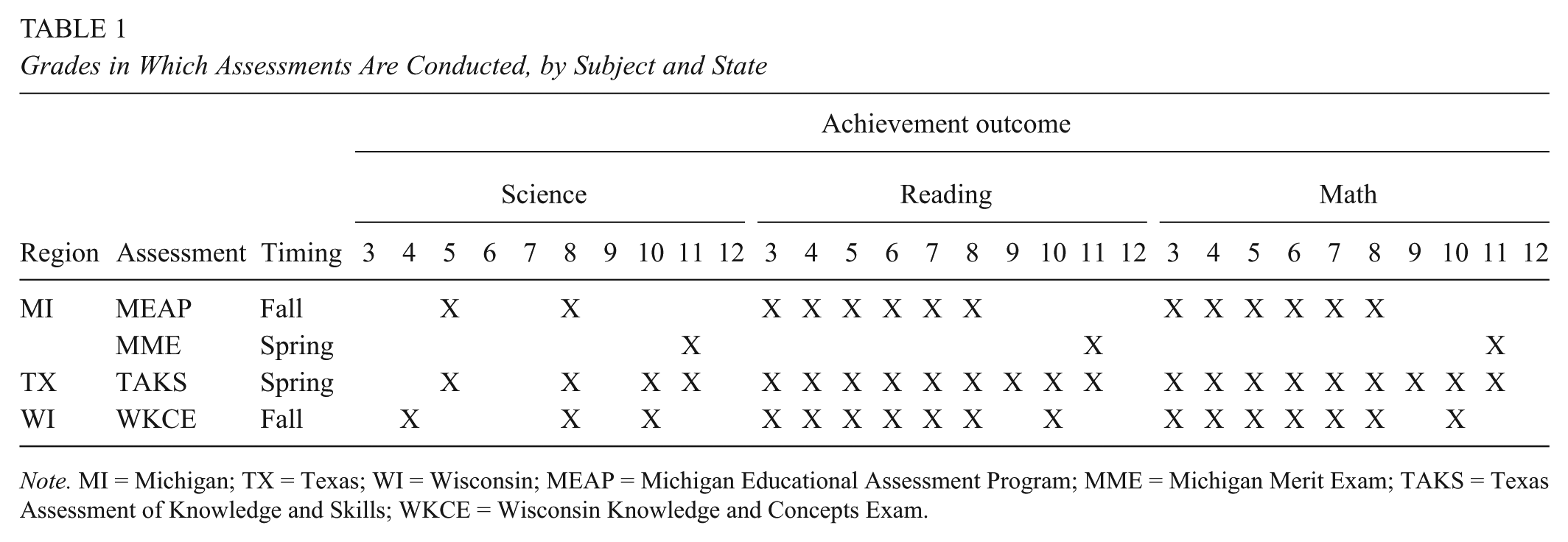
Note. MI = Michigan; TX = Texas; WI = Wisconsin; MEAP = Michigan Educational Assessment Program; MME = Michigan Merit Exam; TAKS = Texas Assessment of Knowledge and Skills; WKCE = Wisconsin Knowledge and Concepts Exam.

We prepared each state data set following a similar protocol in order to obtain a consistent set of usable data across years and states. In each state, and for all years of data, we generated indicator variables from a set of demographic variables, including gender, ethnicity, free or reduced-price lunch as a proxy for socioeconomic status (SES), and limited English proficiency (LEP) status. Collectively, the indicator variables for gender, ethnicity, SES, and LEP make up the set of demographic covariates. Students with nonvalid or duplicate student identification numbers, as well as students requiring a testing accommodation (standard or nonstandard) or that were marked as unethical, were removed from the sample. Students with disabilities or identified as receiving special education were also removed. The percentage of data removed for each state during this cleaning process is provided in Table 2. Note that in Texas, the sample size was also reduced by the masking process. In schools with fewer than five individuals in any single demographic group, achievement scores were masked for all students in that group.

Table 2

Counts of Students, Schools, and Districts for Science Achievement Unconditional Models, by Grade, State, and Year

	Michigan				Wisconsin				Texas
Year	% Data removed by cleaning	Total students	Total schools	Total districts	% Data removed by cleaning	Total students	Total schools	Total districts	% Data removed by cleaning	% Cleaned data that is masked	Total students	Total schools	Total districts
Grade 4
2005-2006					16.0	50,502	1,127	426
2006-2007					15.6	50,173	1,114	424	16.4	22.5	215,443	3,414	932
2007-2008					15.5	50,894	1,114	426	20.2	22	216,480	3,497	947
2008-2009					15.4	51,174	1,115	427	20.1	21.7	221,713	3,581	955
2009-2010					15.5	52,025	1,110	427	19	28.1	210,770	3,625	954
2010-2011					15.4	51,928	1,098	427	20	26.7	218,712	3,681	952
Grade 5
2005-2006									15.8	13.2	247,800	1,601	934
2006-2007	15.0	100,319	2,105	735					16.8	12.9	241,312	1,610	926
2007-2008	15.0	99,553	2,063	735					16.5	12.4	252,122	1,646	943
2008-2009	14.9	98,478	2,188	750					15.3	17.4	242,141	1,664	937
2009-2010	13.1	101,640	2,121	746					15.9	16.2	249,608	1,704	942
Grade 8
2005-2006					16.2	56,217	633	426
2006-2007					16.0	55,180	620	422	16.8	11.5	235,828	1,279	931
2007-2008	14.0	108,046	1,166	721	15.9	54,100	622	424	17.2	11.7	236,411	1,312	944
2008-2009	14.5	105,034	1,127	722	15.0	53,095	624	426	16.3	11.3	241,548	1,324	941
2009-2010	13.9	102,497	1,592	731	15.1	52,572	632	428	15.7	15.9	231,799	1,329	923
2010-2011	12.6	104,679	1,219	736	14.4	52,683	628	429	16.8	14.3	239,716	1,348	925
Grade 10
2005-2006					14.8	60,908	541	386
2006-2007					16.9	60,196	520	382	15.9	11.4	206,076	1,229	894
2007-2008					16.7	59,148	534	383	15.6	11.5	208,188	1,254	908
2008-2009					16.2	58,288	537	383	14.8	11.2	218,876	1,307	930
2009-2010					16.0	57,533	535	382	14.2	15.4	216,260	1,321	917
2010-2011					15.2	56,610	531	381	15.9	14.3	217,526	1,326	899
Grade 11
2007-2008	16.6	104,236	949	614
2008-2009	16.2	102,396	954	622
2009-2010	16.1	99,946	950	629
2010-2011	13.4	102,944	1,044	625

Models

We empirically estimate ICCs and R²s using two models. First, we use a two-level hierarchical model with students nested within schools. Next, we use a three-level hierarchical model with students nested within schools nested within districts.

The design parameter estimates from the two models serve to inform different designs. Estimates from the two-level model directly inform the design of a schoolwide intervention study where students are nested within schools and whole schools are randomly assigned to treatment conditions. Estimates from the three-level model directly inform the design of a districtwide intervention study where students are nested within schools that are nested within districts and whole districts are randomly assigned.

We first present the unconditional two- and three-level models, which do not include covariates, to show the ICC calculations. This is followed by an example of the two-level conditional models, which include covariates, to show the calculations for the R²s. The three-level model with covariates is a direct extension of the two-level model and is therefore not included.

Two-Level Unconditional Model

For each grade and data set, we begin with an unconditional model. Following the Raudenbush and Bryk (2002) notation, the Level 1 model is

Y_{i j} = β_{0 j} + r_{i j}, r_{i j} ~ N (0, σ^{2}),

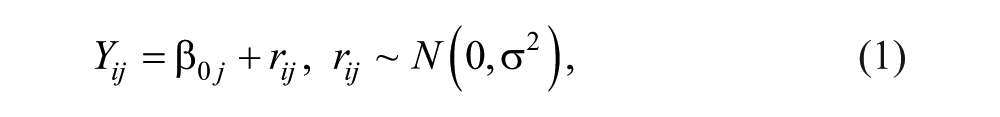
for i ∈ {1, 2, . . . , n} persons per cluster j ∈ {1, 2, . . . , J} clusters, where Y_ij is the outcome for person i in cluster j, β_0j is the mean for cluster j, r_ij is the error associated with each person, and σ² is the within-cluster variance. The Level 2 model, or cluster-level model, is

β_{0 j} = γ_{00} + u_{0 j}, u_{0 j} ~ N (0, τ_{00}),

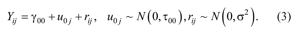
where γ₀₀ is the grand mean, u_0j is the random effect associated with each cluster, and τ₀₀ is the variance between clusters. The mixed model is

Y_{i j} = γ_{00} + u_{0 j} + r_{i j}, u_{0 j} ~ N (0, τ_{00}), r_{i j} ~ N (0, σ^{2}) .

The ICC (ρ) and corresponding standard error for a large, balanced (i.e., an equal number of students per school) sample are

ρ = \frac{τ_{00}}{τ_{00} + σ^{2}} S E (ρ) = \sqrt{\frac{{(1 - ρ)}^{2} v_{2}}{{(σ^{2} + τ_{00})}^{2}}}

where v₂ is the variance of the estimate of τ₀₀ (Donner & Koval, 1982; Hedges, Hedberg, & Kuyper, 2012).

Three-Level Unconditional Model

The three-level model is a natural extension of the two-level model; hence, we omit the presentation of each level individually and present only the mixed model. The unconditional mixed model is

\begin{array}{l} Y_{i j k} = γ_{000} + u_{00 k} + r_{0 j k} + e_{i j k}, \\ u_{00 k} ~ N (0, τ_{β}), r_{0 j k} ~ N (0, τ_{π}), e_{i j k} ~ N (0, σ^{2}) . \end{array}

Note that in a three-level model, there are two ICCs because there are three variance components. Following Hedges et al. (2012), the Level 2 and Level 3 ICC and corresponding standard error—assuming a large, balanced (i.e., an equal number of students per school) sample—are

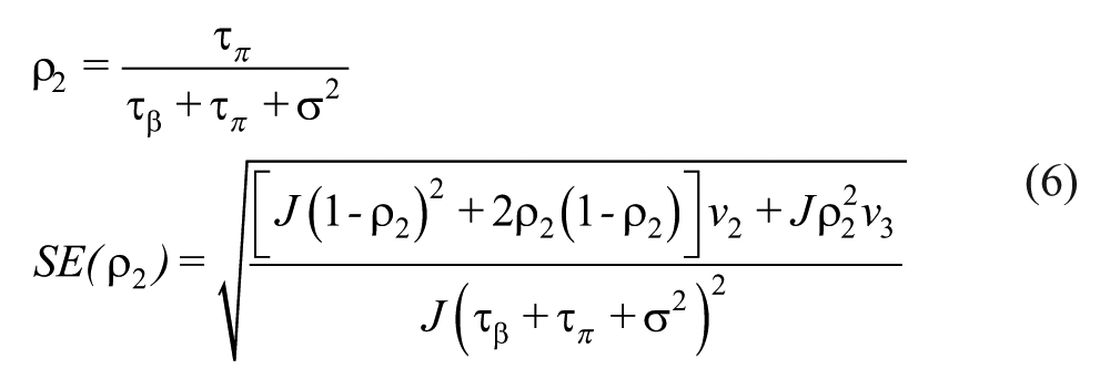
\begin{array}{l} ρ_{2} = \frac{τ_{π}}{τ_{β} + τ_{π} + σ^{2}} \\ S E (ρ_{2}) = \sqrt{\frac{[J {(1 - ρ_{2})}^{2} + 2 ρ_{2} (1 - ρ_{2})] v_{2} + J ρ_{2}^{2} v_{3}}{J {(τ_{β} + τ_{π} + σ^{2})}^{2}}} \end{array}

\begin{array}{l} ρ_{3} = \frac{τ_{β}}{τ_{β} + τ_{π} + σ^{2}} \\ S E (ρ_{3}) = \sqrt{\frac{[J ρ_{3}^{2} + 2 ρ_{3} (1 - ρ_{3})] v_{2} + J {(1 - ρ_{3})}^{2} v_{3}}{J {(τ_{β} + τ_{π} + σ^{2})}^{2}}} \end{array}

where v₂ and v₃ are the variances of the estimate of τ_π and τ_β, respectively, and J is the harmonic mean number of schools per district.

Two-Level Conditional Models

In order to explain the variance in the outcome and obtain a more precise estimate of the treatment effect, we include covariates. Depending on the availability of data, covariates can occur at Level 1 or Level 2. In this study we consider covariates at both Level 1 and Level 2. We do not center the covariates in our models as the choice of centering will not impact the estimates of the variance components in the models we consider. However, it is important to note that in analyses that seek to estimate the effect of an intervention, centering does impact the coefficients and interpretation of these estimates. In cases when we use a student-level covariate, the aggregated covariate at the school level (school mean) is also included. The Level 1 covariates we consider include student-level pretests and student-level demographics, such as gender or free/reduced-price lunch status. We also explored cases with no Level 1 covariate and only a Level 2 covariate, such as school mean scores from the previous year, as a previous year’s school mean is a common covariate used in the design of CRTs (Bloom, Richburg-Hayes, & Rebeck-Black, 2007).

For illustration purposes, we provide the models that include both student-level covariates at Level 1 and the corresponding aggregate school-level covariates at Level 2. The models easily extend to cases with covariates at only higher levels and to three-level models. Building from Equation (1), the Level 1 model with student-level covariates can be written as

Y_{i j} = β_{0 j} + \sum {{}_{q}β}_{q j} X_{q i j} + r_{i j}, r_{i j} ~ N (0, σ_{| X_{Q}}^{2})

for i ∈ {1, 2, . . . , n} persons per cluster j ∈ {1, 2, . . . , J}, clusters, where Y_ij is the outcome for person i in cluster j, β_0j is the adjusted mean for cluster j, X_qij is the value of the q^th student-level covariate for student i in school j, β_qj is the coefficient associated with the q^th covariate for school j, r_ij is the residual error associated with each person conditional on the Q covariates, and $σ_{| X_{Q}}^{2}$ is the residual within-cluster variance.

The new Level 2 model, or cluster-level model, is

β_{0 j} = γ_{00} + \sum {{}_{s}γ}_{0 s} W_{s j} + u_{0 j} u_{0 j} ~ N (0, τ_{| W_{s}})

β_{q j} = γ_{q 0}

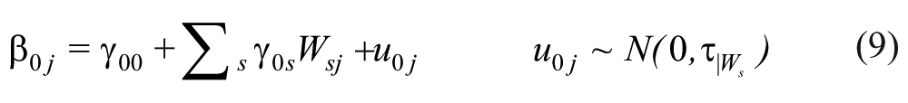
where γ₀₀ is the adjusted grand mean, W_sj is the value of the s^th school-level covariate for school j, γ_0s is the coefficient associated with the s^th school-level covariate; u_0j is the residual error associated with each cluster conditional on the S covariates, and $τ_{| W_{s}}$ is the residual variance between clusters. Note that we assume the Level 1 covariates are fixed and γ_q0 represents the mean coefficient associated with the q^th covariate.

We calculate the proportion of variance explained at Level 1 (R²_L1) and at Level 2 (R²_L2). The R² values are estimated following the procedure of Hedges and Hedberg (2007):

R_{L 1}^{2} = \frac{σ^{2} - σ_{| X_{Q}}^{2}}{σ^{2}} a n d R_{L 2}^{2} = \frac{τ_{00} - τ_{| W_{S}}}{τ_{00}}

Note that if a covariate is included only at Level 2, for example, last year’s school mean, there is no R²_L1 because the Level 1 variance will not be reduced if there is only a Level 2 covariate.

Analyses

As noted in Table 1, each state has its own pattern for testing science. Wisconsin is the only state in our data set that tested in Grade 4. For all other grades, there are a minimum of two states represented, with the exception of Grade 8, in which all three states are applicable. We estimate ICCs for the two-level and three-level models for each data set in each grade. Within each state and grade, we perform a simple average on the ICC estimates and standard errors across the number of years available in the state database.

The R²s we are able to estimate are partially dependent on the specific testing pattern within a state. Table 3 displays the potential covariate sets we explore and identifies the specific data sets that are applicable in each case. For each grade and data set in which we have science test scores, we examine the explanatory power of the set of student demographics, the 1-year lag school-level science scores, the 1-year lag school-level reading scores, and the 1-year lag school-level mathematics scores. Although we could also access the 2- or 3-year school-level lag scores, we do not go beyond the 1-year lag scores since recent work suggests that the strength of the covariates decreases over time (Bloom et al., 2007). Thus, if the 1-year lag school-level scores are available, we do not proceed to the 2-year lag scores. However, for the student-level lag scores, we do not always have a 1-year lag score available and, thus, opt for the most recent student-level lag scores. For the student-level lag scores in a different subject, reading or mathematics, 1-year lag scores are available for Grades 4, 5, and 8 for the states that test in these grades. This is because students are tested in reading and mathematics in the previous grade in each of these cases. However, for the upper grades, 10 and 11, this is not always the case. In Grade 10, the most recent student-level mathematics or reading pretest is a 2-year lag. In Texas, for Grade 11, there is a 1-year student-level lag available in reading and mathematics, since each subject is also tested in Grade 10. In Michigan, the most recent student-level lag using reading or mathematics is a 3-year lag.

Table 3

States in Which Covariate Models for Science Achievement Are Estimated by Grade

		Grade
Covariate	Years lagged	4	5	8	10	11
Demographics	0	WI^f	MI^d, TX^e	MI^d, TX^e, WI^f	TX^e, WI^f	MI^d, TX^e
Most recent school-level pretest
Science	1	WI^e	MI^c, TX^d	MI^c, TX^d, WI^e	TX^d, WI^e	MI^c, TX^d
Reading	1	WI^e	MI^c, TX^d	MI^c, TX^d, WI^e	TX^d, WI^e	MI^c, TX^d
Math	1	WI^e	MI^c, TX^d	MI^c, TX^d, WI^e	TX^d, WI^e	MI^c, TX^d
Most recent student-level pretest
Science	1					TX^d
	2				TX^c, WI^d
	3			MI^a, TX^b		MI^a
	4			WI^b
Reading	1	WI^e	MI^c, TX^d	MI^c, TX^d, WI^e	TX^d	TX^d
	2				WI^d
	3					MI^a
Math	1	WI^e	MI^c, TX^d	MI^c, TX^d, WI^e	TX^d	TX^d
	2				WI^d
	3					MI^a

Note. MI = Michigan; TX = Texas; WI = Wisconsin.

Available for the outcome year 2010-2011.

Available for the two outcome years 2009-2010 and 2010-2011.

Available for the three outcome years 2008-2009 to 2010-2011.

Available for the four outcome years 2007-2008 to 2010-2011.

Available for the five outcome years 2006-2007 to 2010-2011.

Available for the six outcome years 2005-2006 to 2010-2011.

Similar to the ICC analyses, we present a simple average on the R² estimates across the years of data available within each data set. From other empirical work, we would imagine that the 1-year lagged student-level science score would be the strongest covariate (Hedges & Hedberg, 2007). However, this option is available only for Texas at Grade 11. In all other combinations of grades and data sets, the most recent lag science scores is either 2 years (Texas and Wisconsin), 3 years (Michigan and Texas Grade 8), or 4 years (Wisconsin Grade 8) or does not exist (Grades 4 and 5 for any state). Although we considered the model with both demographics and pretests, the additional value of having both was minimal, so in the interest of space, we do not present these results.

Results

We begin with the ICCs for the two- and three-level unconditional models followed by the R² for the different covariate sets.

Intraclass Correlations

Table 4 reports the ICCs for the two-level models for science outcomes. The ICC ranges from a low of 0.172 (Texas Grade 8) to a high of 0.312 (Michigan Grade 11). In other words, in Texas Grade 8, 17% of the variance in science test scores is between schools, whereas it is much higher in Michigan Grade 11, at 31%. In general, the ICC is lower in Texas than in Michigan and Wisconsin for grades in which the three states tested science. Another way of stating this is that there is less variability in science achievement between schools in Texas. We can also look for trends across the grades. In Michigan and Wisconsin, there appears to be more variance between schools (higher ICC estimates) for middle and high school grades than for the elementary grades. However, for Texas, the ICCs were similar across all grades.

Table 4

Unconditional School-Level ICC Averages for Science Achievement Outcomes by Grade and State: Two-Level Model

	Michigan^a		Texas^b		Wisconsin^c
Grade	ICC	SE	ICC	SE	ICC	SE
4					.190	.007
5	.261	.007	.191	.004
8	.261	.009	.172	.005	.256	.012
10			.196	.007	.251	.013
11	.312	.011	.191	.007

Note. ICC = intraclass correlation.

Unconditional ICCs for Michigan are averages across 4 years of data (2007-2008 through 2010-2011).

Unconditional ICCs for Texas are averages across 5 years of data (2006-2007 through 2010-2011).

Unconditional ICCs for Wisconsin are averages across 6 years of data (2005-2006 through 2010-2011).

The unconditional ICCs for the three-level models, students nested in schools nested in districts, are reported in Table 5. The pattern in the ICCs for Texas and Wisconsin is similar. In both states, the school-level variance is always larger than the district-level variance, ranging from almost twice as large to nearly 3 times as large. For example, in Texas in Grade 5, the results suggest that approximately 8% of the variance in science test scores is between districts, 12% is between schools within districts, and the remaining 80% is between students within schools. That is, there is more variability in science achievement between schools within a district than between districts. However, the pattern differs in Michigan. In Grade 5, the ICC at the district level is nearly twice as large as that at the school level, suggesting there is more variability between districts in Michigan than within districts. In Grade 8, the school-level variance and the district-level variance are very similar. And at Grade 11, similar to the other states, there is more variance at the school level than at the district level. However, the order of magnitude is much larger than in other states.

Table 5

Unconditional School-Level and District-Level ICC Averages for Science Achievement Outcomes by Grade and State: Three-Level Model

	Michigan^a				Texas^b				Wisconsin^c
Grade	ICC_L2	SE	ICC_L3	SE	ICC_L2	SE	ICC_L3	SE	ICC_L2	SE	ICC_L3	SE
4									.095	.005	.037	.005
5	.076	.004	.146	.010	.118	.003	.079	.007
8	.102	.009	.117	.011	.104	.005	.060	.007	.107	.008	.036	.006
10					.136	.008	.055	.008	.079	.008	.042	.006
11	.270	.013	.031	.008	.127	.008	.059	.008

Note. ICC = intraclass correlation.

Unconditional ICCs for Michigan are averages across 4 years of data (2007-2008 through 2010-2011).

Unconditional ICCs for Texas are averages across 5 years of data (2006-2007 through 2010-2011).

Unconditional ICCs for Wisconsin are averages across 6 years of data (2005-2006 through 2010-2011).

Percentage of Variance Explained

As identified in Table 3, we examined the strength of the following three sets of covariates: demographics, school-level pretests, and student-level pretests. We present the results in this order since demographics are available for all grades and data sets, school-level pretests are available for all grades, and student-level pretests are less available across the grades and states. The results for the two-level and three-level models are presented in this section.

Table 6 presents the R² values for the set of demographic covariates. Across all grades, databases, and both models, less than 15% of the variance in students’ science test scores within schools is explained by the demographics. In essence, student demographics do not explain a large percentage of the variation in student outcomes within a school. In the two-level model, the explanatory power of the demographics is much larger at the school level. However, the magnitude of the variance explained at the school level seems to vary across states. In Michigan and Wisconsin, the percentage of variance explained by demographics is generally larger than in Texas. In general, within each state, the explanatory power of the demographic covariates does not vary much across grades. A similar pattern holds for the results from the three-level model. In general, there appears to be more consistency across grades within a state and more variability across states with respect to the explanatory power of demographics at the school and district levels.

Table 6

Average R² Values for Demographics Covariates in Two-Level and Three-Level Models by Grade and State

	Two-level HLM^d						Three-level HLM^e
	Michigan^a		Texas^b		Wisconsin^c		Michigan^a			Texas^b			Wisconsin^c
Grade	R ² _L1	R ² _L2	R ² _L1	R ² _L2	R ² _L1	R ² _L2	R ² _L1	R ² _L2	R ² _L3	R ² _L1	R ² _L2	R ² _L3	R ² _L1	R ² _L2	R ² _L3
4					.079	.798							.079	.638	.815
5	.068	.799	.103	.527			.069	.499	.883	.103	.507	.498
8	.073	.782	.134	.615	.106	.842	.073	.554	.885	.134	.663	.458	.107	.625	.889
10			.128	.615	.117	.856				.128	.609	.665	.118	.559	.875
11	.069	.645	.130	.598			.069	.635	.950	.130	.616	.618

Note. HLM = hierarchical linear model.

R² for demographics covariates for Michigan are averages across 4 years of data (2007-2008 through 2010-2011).

R² for demographics covariates for Texas are averages across 5 years of data (2006-2007 through 2010-2011).

R² for demographics covariates for Wisconsin are averages across 6 years of data (2005-2006 through 2010-2011).

The two-level model refers to a conditional HLM with students nested in schools. Student demographic covariate variable set is included at Level 1 and aggregated at Level 2.

The three-level model refers to a conditional HLM with students nested in schools nested in districts. Student demographic covariate variable set is included at Level 1 and aggregated at Level 2 and Level 3.

We present the results for the school-level pretests for science, reading, and mathematics in Table 7. Note that because these are school-level covariates, variation at the student level cannot be explained. We begin by comparing the results by subject of the pretest for the two-level model. For example, in Grade 5 in Michigan, the percentage of variance explained by the school-level science pretest is higher than for the reading or mathematics pretest. In fact, in every grade within each of the three states, the science pretest explains more variability than either the reading or mathematics pretest. This holds in the three-level model as well, where the explanatory power of the school-level science pretest exceeds any other subject pretest at both the school and district level. These findings are similar to recent work that found that same-subject pretests are more powerful than pretests from another subject (Bloom et al., 2007). There also appear to be some trends by state. In each within-grade comparison, the explanatory power of the school-level pretest in Texas, regardless of subject, is less than that of Michigan or Wisconsin, although the magnitude of the difference is small in some cases (i.e., Grade 8 Michigan and Texas.)

Table 7

Average R² Values for Most Recent School-Level Pretest Covariates in Two-Level and Three-Level Models by Subject, Grade, and State

	Two-level HLM^d			Three-level HLM^e
	Michigan^a	Texas^b	Wisconsin^c	Michigan^a		Texas^b		Wisconsin^c
Grade	R ² _L2	R ² _L2	R ² _L2	R ² _L2	R ² _L3	R ² _L2	R ² _L3	R ² _L2	R ² _L3
Science
4			.821					.682	.880
5	.832	.675		.541	.971	.546	.917
8	.837	.802	.908	.642	.946	.739	.856	.817	.844
10		.868	.916			.858	.859	.818	.798
11	.934	.866		.942	.844	.865	.836
Reading
4			.770					.619	.818
5	.764	.582		.416	.918	.472	.713
8	.693	.658	.843	.467	.857	.619	.623	.749	.688
10		.629	.850			.634	.525	.753	.639
11	.876	.584		.893	.743	.583	.586
Mathematics
4			.699					.575	.609
5	.622	.569		.396	.657	.440	.755
8	.717	.671	.782	.509	.780	.630	.617	.682	.567
10		.761	.859			.797	.581	.789	.632
11	.904	.783		.928	.692	.803	.679

Note. HLM = hierarchical linear model

R² for 1-year lagged school-level pretest covariates for Michigan are averages across 3 years of data (2008-2009 through 2010-2011).

R² for 1-year lagged school-level pretest covariates for Texas are averages across 4 years of data (2007-2008 through 2010-2011).

R² for 1-year lagged school-level pretest covariates for Wisconsin are averages across 5 years of data (2006-2007 through 2010-2011).

The two-level model refers to a conditional HLM with students nested in schools. School mean pretest covariates are included at Level 2.

The three-level model refers to a conditional HLM with students nested in schools nested in districts. School mean pretest covariates are included at Level 2 and aggregated at Level 3.

The results for the most recent student-level pretest from each of the three subjects are in Table 8. It is important to keep in mind that the lag on the pretest may be 1, 2, 3, or even 4 years depending upon the specific state, grade, and pretest of interest. Thus, we cannot do a simple comparison within each state or within a grade, as we did in previous tables. However, there are several comparisons to consider. First, we can examine the R² for the different subjects with the same-length lag. For example, in Michigan in Grade 11, a 3-year lag is the first available student-level lag for science, reading, and mathematics. For each subject in the two- and three-level models, the science pretest explains more variability than the reading or mathematics pretest at the student, school, and district levels. The pattern can also be tested by examining the 1-year lag for Texas at Grade 11, which is available for all subject areas, as well as the 2-year lag for Wisconsin at Grade 10. In each of these cases, the science pretest explains more variance at the top level of the model than the pretest in any other subject. It is also important to note that for the first grade science is tested, typically Grade 4 or 5, a student-level science pretest will not be available.

Table 8

R² Values for Most Recent Student-Level Pretest Covariates in Two-Level and Three-Level Models by Subject, Grade, and State

	Two-level HLM^d						Three-level HLM^e
	Michigan^a		Texas^b		Wisconsin^c		Michigan^a			Texas^b			Wisconsin^c
Grade	R ² _L1	R ² _L2	R ² _L1	R ² _L2	R ² _L1	R ² _L2	R ² _L1	R ² _L2	R ² _L3	R ² _L1	R ² _L2	R ² _L3	R ² _L1	R ² _L2	R ² _L3
Science
4
5
8	.413	.797	.297	.640	.418	.868	.413	.693	.783	.297	.630	.565	.418	.789	.744
10			.470	.806	.537	.899				.470	.817	.740	.537	.803	.777
11	.450	.881	.505	.912			.450	.904	.774	.505	.903	.922
Reading
4					.526	.836							.527	.727	.875
5	.429	.846	.268	.634			.429	.598	.944	.268	.558	.713
8	.419	.835	.319	.745	.515	.911	.419	.677	.895	.319	.758	.605	.515	.829	.830
10			.167	.664	.377	.682				.167	.688	.550	.446	.804	.634
11	.273	.815	.191	.707			.273	.825	.761	.191	.678	.729
Mathematics
4					.453	.760							.453	.662	.676
5	.400	.736	.270	.628			.400	.529	.789	.270	.522	.747
8	.441	.761	.413	.754	.436	.828	.441	.580	.784	.413	.714	.741	.436	.763	.560
10			.439	.839	.368	.643				.439	.865	.718	.462	.758	.532
11	.419	.832	.445	.817			.419	.873	.654	.445	.827	.758

Note. HLM = hierarchical linear model.

Most recent student-level science pretest covariate for science achievement outcome in Grades 8 and 11 for Michigan is a 3-year lag; R² represents 1 year of data (2010-2011). Most recent student-level reading and mathematics pretest covariates for science achievement outcomes in Grades 5 and 8 for Michigan are a 1-year lag; R² represents an average of 3 years of data (2008-2009 through 2010-2011). Most recent student-level reading and mathematics pretest covariates for science achievement outcome in Grade 11 for Michigan are a 2-year lag; R² represents an average of 2 years of data (2009-2010 through 2010-2011).

Most recent student-level science pretest covariate for science achievement outcome in Grade 8 for Texas is a 3-year lag; R² represents average across 2 years of data (2009-2010 through 2010-2011). Most recent student-level science pretest covariate for science achievement outcome in Grade 10 for Texas is a 2-year lag; R² represents average across 3 years of data (2008-2009 through 2010-2011). Most recent student-level science pretest covariate for science achievement outcome in Grade 11 for Texas is a 1-year lag; R² represents average across 4 years of data (2007-2008 through 2010-2011). Most recent student-level reading and mathematics pretest covariates for science achievement outcomes in Grades 5, 8, and 11 for Texas are a 1-year lag; R² represents average across 4 years of data (2007-2008 through 2010-2011).

Most recent student-level science pretest covariate for science achievement outcomes in Grade 8 for Wisconsin is a 4-year lag; R² represents average across 3 years of data (2008-2009 through 2010-2011). Most recent student-level science pretest covariate for science achievement outcome in Grade 10 for Wisconsin is a 2-year lag; R² represents averages across 5 years of data (2007-2008 through 2010-2011). Most recent student-level reading and mathematics pretest covariates for science achievement outcomes in Grades 5 and 8 for Wisconsin are a 1-year lag; R² represents averages across 6 years of data (2006-2007 through 2010-2011). Most recent student-level reading and mathematics pretest covariates for science achievement outcome in Grade 10 for Wisconsin is a 2-year lag; R² represents averages across 5 years of data (2007-2008 through 2010-2011).

The two-level model refers to a conditional HLM with students nested in schools. Student-level pretest covariate is included at Level 1 and aggregated at Level 2.

The three-level model refers to a conditional HLM with students nested in schools nested in districts. Student-level pretest covariate is included at Level 1 and aggregated at Level 2 and Level 3.

It is also interesting to examine the explanatory power in the case when the time lag for a science pretest is greater than the time lag for a reading or mathematics pretest. For example, in Grade 8 in Michigan and Texas, the first available time lag for a science pretest is 3 years. However, the mathematics and reading pretests for Grade 8 are available at 1 year. In the majority of the cases, the 1-year lag mathematics or reading pretest options explained more variation at the student, school, or district level than the 3-year lag science pretest. Given that in many cases the 1-year lag from a different subject had more explanatory power and may be more accessible than the 3-year lag of the same subject, it seems reasonable to consider the shorter lag for a different subject pretest as a viable covariate to increase the power of a study.

Looking Across Covariate Sets

We presented R² values from three different types of covariate sets: demographics, school-level pretests, and student-level pretests. Looking across Tables 6 through 8, we can compare the explanatory power of the different covariate sets. In the one case in which a 1-year lag student-level science pretest was available (Texas in Grade 11), it explains more variance than any other covariate set at the school level and district level (in the case of the three-level model). In all other cases, the explanatory power of the 1-year lag school-level science pretest was greater than any other student-level pretest or the set of demographics. Given the fact that science is not typically tested annually and hence it is rare that there is a 1-year lag student-level science pretest available, the 1-year lag school-level science pretest is often the best option.

In addition to the empirical estimates of the R², which support the use of the 1-year lag school-level science pretest, there are other factors that also lead to this covariate set as a strong option. First, although the student-level pretest does explain variation at the student level, the key variation in a CRT that needs to be explained to increase the power of the study is at the level of randomization. Hence, more weight should be given to the covariate set that explains the most variation at Level 2 in a two-level design or Level 3 in a three-level design, unless the number of units at this level is small. Konstantopoulos (2012) notes that the decrease in degrees of freedom resulting from adding a covariate at the level of randomization can reduce statistical power. Second, individual students’ past-year test scores and demographics may be costly to obtain, whereas school-level pretest scores may be more readily available from the school administrators or a website. This will help reduce costs, a critical factor, since CRTs are often very expensive (Konstantopoulos, 2009). Next we provide two applications of how these empirical estimates can be used in the design of a two-level CRT.

Applications

The design parameters in Tables 4 through 8 can be used in planning science impact studies. Suppose that a team of science researchers are designing a study to test the efficacy of a new science curriculum for fifth graders in the state of Michigan. They plan to randomly assign entire schools to either the new curriculum or the current curriculum. There are approximately 125 fifth graders per school. Given the budgetary constraints of the project, the team is limited to 40 schools and plans to randomly assign half to treatment and half to the comparison group. The team has a fixed number of schools, which is common in practice, given access to schools and budgetary constraints (Taylor et al., 2013). Hence the goal of the power analysis is to determine the smallest effect than has an 80% chance of being found to be statistically significant, also known as the minimum detectable effect size (MDES; Bloom, 1995). Then the team can evaluate whether the MDES is reasonable, given the intervention being tested.

Determining whether the MDES is appropriate is not an easy task. Based on a review of 76 meta-analyses of studies of educational interventions, Hill, Bloom, Rebeck-Black, and Lipsey (2008) found mean treatment effect sizes in the 0.20-to-0.30 range. For science interventions, the Slavin et al. (2014) review of elementary science programs found average treatment effects ranging from 0.03 to 0.42. Although larger effect sizes are appealing to researchers because they require fewer clusters, it is important to think through the ramifications of designing a study with too large of an MDES. For example, suppose that a study is designed to detect an MDES of 0.40. This means that the study has adequate power to detect an effect of 0.40 or higher, but it is not powered to detect an effect smaller than 0.40. Hence if the true effect is in the range noted by Hill et al., the study would be underpowered and the researchers may incorrectly conclude that the treatment had no effect.

For the power analysis, assume that the researchers use Optimal Design Plus (OD Plus; Raudenbush et al., 2011) to calculate the MDES. Estimates of the ICC and R² are necessary input parameters for calculating the MDES. Given that they are working with fifth graders in Michigan and the results in Table 4 include estimates for a two-level model for fifth graders from Michigan, they estimate an ICC of 0.261. Next, the researchers must choose which covariate set they plan to use. Looking through Tables 6 through 8 for specific estimates for Michigan Grade 5, the options include student demographics; 1-year lag school-level pretest for science, reading, or mathematics; and 1-year lag student-level pretest for mathematics or reading. The explanatory power of the covariate sets at the school level for the different options range from 0.622 up to 0.846. Note that the higher the explanatory power of the covariate(s), the smaller the MDES. However, differences in the MDES for a covariate that explains 82% of the variance compared to 84% of the variance will be minimal, and other factors should also be considered. In this case, approximately 83.2% of the variance in science test scores can be explained with the previous year’s school-level pretest. The only covariate set with greater explanatory power is the 1-year lag student-level reading test at 84.6%. The difference in explanatory power of these two covariates is small compared to the potential difference in the cost of obtaining these two sets of covariates. School-level science scores from the previous year are likely available via a website or very quickly from a school administrator. Individual student test score data from the previous year may be much more time-consuming and costly to obtain for all schools, if available at all. Thus, from a statistical and practical perspective, it makes sense to use the 1-year lag school-level science scores. Using OD Plus, assuming 20 schools per condition, 125 students per school, an ICC of 0.261, and an R² of 0.832, the MDES is 0.202. In other words, the study is powered at 0.80 to detect an effect of 0.202, at the lower end of the range suggested by Hill et al. (2008).

In the first application, the study location and the study design matched exactly to the information provided by our analyses. Naturally, this will not always be the case. In other scenarios, the desired design may be different. For example, the classroom level may be included in the study, making the levels of nesting different, or schools may be blocked by district, resulting in a multisite cluster randomized trial (MSCRT) with districts as sites. Similarly, a different state or specific subset of schools within a specific state may be included in the study. The study may also involve a different grade that our current estimates do not cover. Although our results will not directly match the needs of every impact study design, we argue they can still provide useful information for evaluating estimates of design parameters. Without estimates that align exactly with the proposed study, it is incumbent upon the researcher to cautiously utilize any available information to craft the best argument possible for selecting design parameter estimates.

For example, suppose that the new fifth-grade science curriculum also had an eighth-grade curriculum. The research team wants to test the efficacy of the eighth-grade curriculum and plans to conduct a two-level CRT with students nested within schools. The budget allows for a total of 30 schools, 15 in the treatment condition and 15 continuing with the current science curriculum, and 300 kids per school. The team plans to recruit schools from the state of Ohio. The researchers want to know the MDES, given the current size of the study.

In this case, the estimates of the design parameters in Tables 4 through 8 do not directly match since the estimates for Ohio are not included in the tables. However, the design parameters can still be used to guide the estimates. One option is to examine the student population in Ohio and the configuration of the schools and districts to try to determine if Ohio is more similar to any of the three states included in our analyses. This might include an examination of things like average district size, prior achievement, percentage free/reduced-price lunch, percentage minority, and so on. In many cases, these data are available through state-specific websites or the Common Core of Data (www.ncer.ed.gov/ccd/). If Ohio seems similar to any of the three states in the tables, the research team could make a case to use empirical estimates from that state. However, caution is advised, as without further examples of estimates from other states, it is unknown which factors are the most essential to consider when comparing states. An additional option is to use a point estimate (e.g., the mean, weighted mean, median, or lower/upper bound of the estimated confidence interval) across states of the design parameters presented in this article. In this scenario, it is important to consider the representativeness of these three states, as it is unknown, for example, whether any of the three states constitutes an extreme case. For illustrative purposes, we will select the (simple) mean ICC value, 0.230, for our example power calculation.

The choice of covariate sets also needs to be considered. Looking across Tables 6 through 8 at Grade 8, it appears that the percentage of variance explained by the student-level pretests is very similar to that of the school-level science pretests. Given the additional time and cost to collect student-level pretests, we proceed with the previous year’s school-level science scores (Table 7). Similar to the ICC, we might choose to justify a point estimate for the percentage of variance explained by the school-level pretest. Across the three states, the mean value is 0.849. Combining the mean ICC with the mean percentage of variance explained by the school-level pretest, we can calculate the MDES. In this case, the MDES estimate is 0.205.

Discussion

Across education, there is an emphasis on rigorous research to test the impact of programs and practices. Some argue that science education lags behind other fields in responding to this call (e.g., Minner, Levy, & Century, 2010; Slavin et al., 2014). However, given the recent release of the Guidelines and the federal emphasis on impact studies for determining the effectiveness of educational interventions, we expect that we will continue to see more science education impact studies. It is critical that all impact studies be well designed and adequately powered to yield high-quality evidence of program effectiveness. In order to design adequately powered impact studies of science interventions, teams planning these studies must estimate design parameters to use in the power analyses. This article seeks to improve the accuracy of the power calculations by providing empirical estimates of design parameters for impact studies with science education outcomes. In this article, we focused on the decomposition of the variance in science test scores between districts and schools and the explanatory power for different covariate sets for planning two- and three-level CRTs.

In terms of the variance in science test scores between schools and districts, the empirical estimates suggest these estimates vary across states. On average, the estimates of the between-school and between-district variance from Texas were lower than both Wisconsin and Michigan. The variance between schools and between districts also appeared to vary across grades, with higher grades tending to have higher values. However, this pattern was not consistent across all states, and adding more states to the database would be helpful in testing this pattern.

We examined the empirical estimates of the percentage of variance explained along three dimensions: demographics, school-level pretests, and student-level pretests. In general, the explanatory power of the 1-year lag school-level science pretest was the highest. Given that school-level pretests are much less expensive and easier to obtain than student-level demographics or pretests, we suggest use of the 1-year lag school-level science scores.

The empirical estimates of design parameters provided in this article are meant to serve as a resource and a guide to designing impact studies. In any particular study, the true values of the design parameters may be different than the estimated values. For example, the estimates for each state take into account all schools in the state. However, if the schools were selected from one large district within a state, the schools within that district may be more homogeneous than the schools across the entire state. Hence, characteristics of the sample of schools and the design itself should be considered when selecting the most appropriate design parameters.

The extant empirical work into design parameters for science education impact studies is minimal compared to that focused on reading and mathematics education outcomes. Yet impact studies focused on science education outcomes are held to the same standards as those focused on reading and mathematics education outcomes. If rigorous evidence of the impact of science education interventions is to accumulate and accumulate quickly, as suggested in the Guidelines document, science education researchers should seek to design studies that can detect substantively important effects. Hence, building a resource of design parameters specific to science education is a critical step toward moving forward the agenda to improve the rigor of impact studies in the field.

Future Directions

To date, the current article represents the largest set of design parameters for teams planning impact studies focused on improving science outcomes. We see this as the beginning of a resource for science education researchers planning such studies. However, there are several ways this resource can continue to grow.

One strategy is to encourage research teams to report the variance components and percentage of variance explained from covariate sets. Coupled with details on the sample of schools in the study, this may provide a useful resource for a team planning a similar study with a similar set of schools.

A second strategy is to update the design parameter estimates with additional states and databases. Adding states and other databases may help elucidate the between-state patterns and clarify the potential trend toward more between school variance in the upper grades.

A third extension is to consider additional designs. In science education, it is becoming more common to design studies to involve the teacher level. This includes three-level CRTs with students nested within teachers nested within schools and treatment assigned at the school level as well as MSCRTs with students nested within teachers and teachers assigned to treatment within schools (Heller et al., 2012). Hence, estimating design parameters that include the teacher level is important.

With the emergence of three-level CRTs that include a teacher level, estimating design parameter for studies with teacher outcomes of knowledge or practice become a fourth possible research focus in their own right. Recently, Kelcey and Phelps (2013) estimated design parameters for teacher outcomes related to mathematics and reading content knowledge and practice and found they differed from student outcomes. In fact, there was more clustering for teacher-level outcomes than for student-level outcomes. However, to date, there are no studies reporting design parameters relative to teacher-level outcomes for science.

Finally, the literature base would be enriched by future studies that explore why clustering effects can be quite strong and what variables might cause them to differ. For example, it is somewhat intuitive to posit that between-state differences in the percentage of variance at the school and district levels could be related to the fact that “neighborhood effects” are stronger in some states than others—more specifically, that student or school demographics are clustered differently across states (e.g., as a result of the state or local political, cultural, or economic conditions) and those demographic variables are strongly associated with outcomes. However, this explanation is not consistent with our observation that there is more variance between schools on science outcomes at high school than at elementary school. If the neighborhood effect were the only factor at play, then we might expect greater between-school variance for elementary schools than for high schools, as elementary schools tend to draw from a small number of adjacent neighborhoods and high schools tend to draw from a larger number of scattered neighborhoods with presumably more demographic diversity. This was not the case in this study. Perhaps there is a factor related to the high school curriculum or culture that results in students being more similar in achievement to their classmates than to other high school students, and this factor is less pronounced in elementary schools. Furthermore, it seems possible that differences in the psychometric properties associated with the various state tests (across or even within states) could account for some of the variability in design parameters that we find across populations and grades. In summary, we suspect that the design of CRTs would benefit greatly from a set of rigorous explorations of these interrelated phenomena.

Footnotes

Funding

This work was funded by the National Science Foundation, Award 1118555.

Authors

JESSACA SPYBROOK is an associate professor in the Department of Educational Leadership, Research, and Technology at Western Michigan University. Her research focuses on improving the quality of the designs and power analyses of cluster randomized trials in education.

CARL D. WESTINE is an assistant professor in the College of Education at the University of West Georgia. His research focuses on the improving the efficiency of evaluations, particularly in education.

JOSEPH A. TAYLOR is a principal associate/scientist at Abt Associates. His background is in science education research with an emphasis on meta-analysis, statistical reporting practices, and the design of causal effect studies.

References

Bloom

H. S.

(1995). Minimum detectable effects: A simple way to report the statistical power of experimental designs. Evaluation Review, 19(5), 547-556.

Bloom

H. S.

Bos

J. M.

Lee

S. W.-Y.

(1999). Using cluster random assignment to measure program impacts. Evaluation Review, 23(4), 445-469.

Bloom

H. S.

Richburg-Hayes

Rebeck-Black

(2007). Using covariates to improve precision for studies that randomize schools to evaluate educational interventions. Educational Evaluation and Policy Analysis, 29(1), 30-59.

Brandon

P. R.

Harrison

G. M.

Lawton

B. E.

(2013). SAS code for calculating intraclass correlation coefficients and effect size benchmarks for site-randomized education experiments. American Journal of Evaluation, 34(1), 85-90.

Donner

Koval

J. J.

(1982). Design considerations in the estimation of intraclass correlation. Annals of Human Genetics, 46(3), 271-277.

Hedberg

E. C.

Hedges

L. V.

(2014). Reference values of within-district intraclass correlations of academic achievement by district characteristics: Results from a meta-analysis of district specific values. Evaluation Review, 38(6), 546-582.

Hedges

L. V.

Hedberg

E. C.

(2007). Intraclass correlation values for planning group-randomized trials in education. Educational Evaluation and Policy Analysis, 29(1), 60-87.

Hedges

L. V.

Hedberg

E. C.

(2013). Intraclass correlations and covariate outcome correlations for planning two- and three-level cluster randomized experiments in education. Evaluation Review, 37(6), 445-489.

Hedges

L. V.

Hedberg

E. C.

Kuyper

A. M.

(2012). The variance of intraclass correlations in three- and four-level models. Educational and Psychological Measurement, 72(6), 893-909.

10.

Heller

J. I.

Daehler

K. R.

Wong

Shinohara

Miratrix

L. W.

(2012). Differential effects of three professional development models on teacher knowledge and student achievement in elementary science. Journal of Research in Science Teaching, 49(3), 333-362.

11.

Hill

C. J.

Bloom

H. S.

Rebeck-Black

Lipsey

M. W.

(2008). Empirical benchmarks for interpreting effect sizes in research. Child Development Perspectives, 2(3), 172-177.

12.

Institute of Education Sciences & National Science Foundation. (2013). Common guidelines for education research and development. Retrieved from http://ies.ed.gov/pdf/CommonGuidelines.pdf

13.

Jacob

Zhu

Bloom

H. S.

(2010). New empirical evidence for the design of group randomized trials in education. Journal of Research on Educational Effectiveness, 3(2), 157-198.

14.

Kelcey

Phelps

(2013). Considerations for designing group randomized trials of professional development with teacher knowledge outcomes. Educational Evaluation and Policy Analysis, 35(3), 370-390.

15.

Konstantopoulos

(2009). Incorporating cost in power analysis for three-level cluster-randomized designs. Evaluation Review, 33(4), 335-357.

16.

Konstantopoulos

(2012). The impact of covariates on statistical power cluster-randomized designs: Which level matters more? Multivariate Behavioral Research, 47(3), 392-420.

17.

Lee

Krajcik

(2012). Large-scale interventions in science education for diverse student groups in varied educational setting. Journal of Research in Science Teaching, 49(3), 271-280.

18.

Lynch

S. J.

Pyke

Grafton

B. H.

(2012). A retrospective view of a study of middle school science curriculum materials: Implementation, scale-up, and sustainability in a changing policy environment. Journal of Research in Science Teaching, 49(3), 305-332.

19.

Minner

D. D.

Levy

A. J.

Century

(2010). Inquiry-based science instruction: What is it and does it matter? Results from a research synthesis years 1984-2002. Journal of Research in Science Teaching, 47(4), 474-496.

20.

Penuel

W. R.

Fishman

B. J.

(2012). Large-scale science education intervention research we can use. Journal of Research in Science Teaching, 49(3), 281-304.

21.

Plass

J. L.

Milne

Homer

B. D.

Schwartz

R. N.

Hayward

E. O.

Jordan

Barrientos

(2012). Investigating the effectiveness of computer simulations for chemistry learning. Journal of Research in Science Teaching, 49(3), 394-419.

22.

Raudenbush

S. W.

Bryk

A. S.

(2002). Hierarchical linear models: Applications and data analysis methods (2nd ed.). Thousand Oaks, CA: Sage.

23.

Raudenbush

S. W.

Spybrook

Congdon

Liu

Martinez

Bloom

Hill

(2011). Optimal design software plus empirical evidence (Version 3.0) [Software]. Retrieved from http://www.wtgrantfoundation.org

24.

Schochet

P. Z.

(2008). Statistical power for random assignment evaluations of education programs. Journal of Educational and Behavioral Statistics, 33(1), 62-87.

25.

Shadish

W. R.

Cook

T. D.

Campbell

D. T.

(2002). Experimental and quasi experimental designs for generalized causal inference. Boston, MA: Houghton Mifflin.

26.

Slavin

R. E.

Lake

Hanley

Thurston

(2014). Experimental evaluations of elementary science programs: A best-evidence synthesis. Journal of Research in Science Teaching, 51(7), 870-901.

27.

Spybrook

Raudenbush

S. W.

(2009). An examination of the precision and technical accuracy of the first wave of group randomized trials funded by the Institute of Education Sciences. Educational Evaluation and Policy Analysis, 31(3), 298-318.

28.

Taylor

Kowalski

Wilson

Getty

Carlson

(2013). Conducting causal effect studies in science education: Considering methodological trade-offs in the context of policies affecting research in schools. Journal of Research in Science Teaching, 50(9), 1127-1141.

29.

Westine

Spybrook

Taylor

(2013). An empirical investigation of design parameters for planning cluster randomized trials of science achievement. Evaluation Review, 37(6), 490-519.

30.

Nichols

(2010). New estimates of design parameters for clustered randomization studies: Findings from North Carolina and Florida. Washington, DC: Urban Institute, National Center for Analysis of Longitudinal Data in Education Research.

31.

Zhu

Jacob

Bloom

H. S.

(2012). Designing and analyzing studies that randomize schools to estimate intervention effects on student academic outcomes without classroom-level information. Education Evaluation and Policy Analysis, 34(1), 45-68.

Design Parameters for Impact Research in Science Education

Abstract

Keywords

Statistical Power for CRTs

Design Parameters for Science CRTs

Data

Models

Two-Level Unconditional Model

Three-Level Unconditional Model

Two-Level Conditional Models

Analyses

Results

Intraclass Correlations

Percentage of Variance Explained

Looking Across Covariate Sets

Applications

Discussion

Future Directions

Footnotes

Funding

Authors

References