
Abstract
Research has shown that mathematical proficiency gaps are related to students’ and schools’ indicators of poverty, with fewer studies on neighborhood effects on achievement gaps. Although this literature has accounted for students’ nesting within schools, so far, methodological constraints have not allowed researchers to formally account for multilevel and spatial effects. I contribute to this discussion by simultaneously considering test-takers’ own socioeconomic standing and the impact of their nesting schools and neighborhood structures. Multilevel simultaneous autoregressive (MSAR) models and population-level data of 2.09 million test-takers, whose standardized performances were measured at Grades 3–8 in New York State, revealed the presence of geography of mathematical (dis)advantage. Because mathematical performance is spatially dependent across schools and neighborhoods, moving forward, applied researchers should rely on MSAR to account for sources of spatially driven bias that cannot be handled with multilevel models alone. Full replication code and data are provided at https://cutt.ly/N4zRstL.
Keywords
Introduction
Mathematical proficiency is a gateway to academic and professional success. Mathematical proficiency predicts reading achievement more strongly than early reading performance (Duncan et al., 2007; Farran et al., 2006; Lerkkanen et al., 2005; Pagani et al., 2010) and is a better predictor of later school success than many other academic indicators (Duncan et al., 2007; Wright et al., 2020). Relatedly, given the increasing relevance of science, technology, engineering, and mathematics (STEM) in the globalized economy (González Canché, 2017; Pearman, 2019; Rothwell, 2013), efforts to strengthen students’ mathematical proficiency levels as early as possible would also affect students’ prospects for economic and professional success (Aber et al., 2013; Pearman, 2019).
Mathematical proficiency levels, however, are not homogeneously distributed across student populations. Social-class differences have been consistently documented to influence students’ prospects of mathematical performance as early as preschool and kindergarten (Case et al., 1999; Denton & West, 2002; Starkey et al., 2004). Early competence in mathematics has also been shown to lead to later competence in mathematics, when “children who start ahead in mathematics generally stay ahead” (Siegler et al., 2012, p. 691). Notably, because the effects of mathematical proficiency also lead to success in other academic, economic, and professional areas, early success in mathematics leads to positive spillovers, where success in mathematics begets success in mathematics and in other academic content, thus increasing the possibility of subsequent success in life (Aber et al., 2013). Spillover effects based on mathematical proficiency (or the lack of thereof) can be negative as well, of course, and failure to reach mathematical proficiency in one grade may imply a negative vicious cycle in the learning process of subsequent mathematical topics (Duncan et al., 2007; Siegler et al., 2012; Stevenson & Newman, 1986).
The mechanisms behind the idea that students who start behind in mathematical proficiency tend to remain behind (Siegler et al., 2012) may be explained by the cumulative nature of mathematical knowledge—that is, knowledge gaps in arithmetic foundations pose significant barriers to the learning of derivatives and integrals (Fogarty et al., 2018). In other words, considering this inherently cumulative nature of mathematical knowledge, the negative spillovers of not reaching, or barely reaching, proficiency levels in one grade may impose greater challenges in mastering mathematical content in subsequent grades (Clotfelter et al., 2009). From this point of view, the fact that grade-level proficiency levels may decrease as students advance through grades (e.g., see National Assessment of Educational Progress [NAEP], 2020, 2022) may in part be explained by this cumulative nature but may also be influenced by students’ socioeconomic standing (Case et al., 1999; Denton & West, 2002; Siegler et al., 2012; Starkey et al., 2004). In this respect, although summary indicators of mathematical proficiency are useful in depicting how mathematical proficiency may decrease across grades (Mervosh & Wu, 2022), it remains unclear how these gaps in proficiency levels are expected to vary when simultaneously considering the impact of poverty indicators of students, schools, and even the neighborhoods where those schools are nested or located—that is, it remains much less clear in the academic literature how students from economically disadvantaged backgrounds may fare when they attend schools located in high-poverty neighborhoods or how these same students may be affected when attending schools located in less economically challenged neighborhoods.
Building from research on academic achievement gaps (see Clotfelter et al., 2009; Hanushek & Rivkin, 2006; Phillips & Chin, 2004; Reardon & Galindo, 2009), it is clear that as early as kindergarten, children’s knowledge and skills differ in relation to their families’ socioeconomic indicators (Denton & West, 2002; Duncan et al., 2007; Siegler et al., 2012; Starkey et al., 2004). Although less prevalent in this literature, research has also shown an important association between achievement gaps and place-based socioeconomic disadvantages in the form of neighborhood effects (Considine & Zappalà, 2002; Pearman, 2019). Although this literature has accounted for students’ nesting within schools by relying on multilevel models, so far, methodological constraints have not allowed researchers to formally account for multilevel and spatial or place-based effects on students’ performance while also accounting for these students’ own socioeconomic well-being. To address this gap in the literature, this study aims to offer more nuanced estimates of the magnitudes of expected proficiency changes in mathematics across grade levels by simultaneously considering students’ socioeconomic standing as well as their school-level contexts and place-based poverty levels.
Considering the impact of socioeconomic contexts in mathematical proficiency is relevant because, although the achievement-gap literature has consistently found that as indicators of poverty in a child’s life increase, their academic performance will tend to decline (Considine & Zappalà, 2002; Pearman, 2019), it remains unclear how low-income students attending schools located in wealthier zones perform in mathematical proficiency and how these gaps vary across grades. Similarly, this study assesses how economically disadvantaged students’ performances compare to their non–economically disadvantaged peers attending low-income schools. In sum, this study contributes to research on mathematical competence by modeling changes in mathematical proficiency across grades while simultaneously considering students’ own socioeconomic standing and the impact of their nested school and neighborhood structures.
To meet the goal of this study, I relied on standardized performance records of more than two million test-takers (see Table 3) whose individual mathematical proficiency 1 was reported at the grade level (i.e., not individual records but records aggregated per grade within 3,484 public schools) in Grades 3–8 in the state of New York in the academic years 2017–2018 (3,335 public schools) and 2018–2019 (3,372 public schools), for a total of 3,484 public schools. This administrative data set was complemented with American Community Survey (ACS) indicators and TIGER/Line Shapefiles from the U.S. Census Bureau to build a completely open-access data set (access to replication code and data for all models are available at https://cutt.ly/N4zRstL and in González Canché (2023a)). That accounts for students’, schools’, and neighborhoods’ economic standing to address the following questions, which are captured in the conceptual map in Figure 1:
1. What is the expected change in mathematical proficiency levels observed among students in Grades 3–8? (addressed with Model “Aggregate” in Table 4)
2. How do these proficiency levels vary when considering students’ own levels of economic disadvantage (i.e., receiving at least one form of public assistance 2 ) while simultaneously considering their school-level sociodemographic and economic nesting structures? (addressed with Models 2–7 in Table 4)
This differentiation in mathematical performance by economically disadvantaged status was possible because the administrative records reported by the New York State Education Department (NYSED, 2020b) offered disaggregated proficiency levels in mathematics across schools and within grades by an indicator capturing whether students belonged to the “economically disadvantaged” class—that is, by whether students’ families participated in any form of public assistance (see Table 1).
3. How do performance gaps in mathematical proficiency vary for economically disadvantaged students attending schools located in high-poverty neighborhoods, and how do these gaps compare to those realized by their non–economically disadvantaged peers attending schools located in the least economically challenged neighborhoods? (addressed with Table 3 and Models 2–7 in Table 4)
4. How do other place-based sociodemographic and economic indicators influence the variation of mathematical proficiency? (addressed with Models 1–7 in Table 4)
To address these questions, this study relied on methodological advancements that are yet to be widely implemented in education research (see Dong & Harris, 2015; Dong et al., 2015). The main method of analysis was MSAR models that accounted for the nested structure of the data (i.e., grades nested within schools, schools nested within regions) while also testing for whether spatial dependence was present at the school and region levels and, if so, controlling for those sources of variation. The results indicate that mathematical performance is spatially dependent across schools and neighborhoods. Accordingly, moving forward, applied researchers should consider relying on MSAR to account for sources of spatially driven bias that cannot be handled with multilevel models alone. From this perspective, the distribution of the replication code and data set with this submission is of particular importance for researchers who may want to have access to a fully reproducible example.

Conceptual representation of modeling framework.
Example of Data Structure

As reported by NYSED (2020b).
Outcome of interest. Data retrieved from NYSED (2020b).
The remainder of the paper is organized as follows. It starts with a review of the literature, including the most prevalent strategies that researchers have employed to estimate the variation of mathematical proficiency, considering individual-level attributes, such as ethnicity and socioeconomic status, as well as school and neighborhood effects. It then discusses the conceptual lenses guiding the variable selection as well as indicating hypothetical relationships expected to be observed when considering the literature reviewed and the conceptual framework. Subsequently, the data and methods sections formally discuss MSAR and the relevance of relying on machine learning methods to select predictor and control indicators that remain relevant in the explanation of the main outcome of interest (i.e., mathematical proficiency). This feature or variable selection is particularly important when dealing with place-based indicators that, as described in the conceptual framework section, may be highly correlated. Then, findings are presented, and the paper closes with implications, limitations, and further areas of inquiry that, although important, go beyond the scope of this study (for example, measuring the impact of the COVID-19 pandemic on the academic performance of economically disadvantaged students).
Literature Review
Studies on academic achievement gaps in elementary and middle school education have followed two major trends. The first has focused on studying ethnic and racial gaps to see whether performance gaps have narrowed or expanded among students belonging to different racial/ethnic groups within grades, typically using White students’ academic performance as the reference or comparison group to measure achievement gaps (Clotfelter et al., 2009; Hanushek & Rivkin, 2006; Phillips & Chin, 2004; Reardon & Galindo, 2009). For example, Hanushek and Rivkin (2006) showed that the achievement gap in Grade 1 between Black and White students was 12.3 points, favoring the latter. They then indicated that by Grade 3, this performance gap between Black and White students had increased to 18 points (Hanushek and Rivkin, 2006, p. 10). Similarly, using departures from White students’ performance, Clotfelter et al. (2009) showed that Black-White disparities were the largest among all racial group comparisons in their analytic sample (i.e., comparing White students’ performance with Hispanic, Asian, and American Indian students’ performance). They also showed that in Grade 3, “more than a quarter of [B]lack [students] tested below the 10th percentile of the White distribution” (Clotfelter et al., 2009, p. 408). This result was also observed when using eighth graders’ scores. A consistent modeling strategy employed in these studies is that performance gaps have been measured within grades and between groups.
The second major trend in the achievement gap literature consists of analyzing the association between achievement and socioeconomic disadvantage (Considine & Zappalà, 2002; Pearman, 2019). Indicators of economic distress have been measured at individual students’ family levels as well as at school and neighborhood levels, with results consistently corroborating the negative association between economic disadvantage and academic achievement (Carlson & Cowen, 2015; Pearman, 2019). More to the point, studies have consistently shown that achievement gaps have been present as early as kindergarten (Case et al., 1999; Denton & West, 2002; Starkey et al., 2004), wherein children who start behind remain behind (Duncan et al., 2007; Siegler et al., 2012; Stevenson & Newman, 1986).
With respect to neighborhood and school effects, authors have analyzed these effects on students by standardizing students’ performance across grades—like our data set analyzed herein. For example, Carlson and Cowen (2015) used data from all students attending the Milwaukee Public Schools between 2006–2007 and 2010–2011 who participated in the Wisconsin Knowledge and Concepts Examination. Then they estimated school and neighborhood contributions to 1-year gains in student test scores for elementary and middle school without considering performances within students’ grades, as described above. More recently, Pearman (2019) estimated the effects of neighborhood poverty across children up to age 12. Specifically, Pearman tested the hypothesis that exposure to high-poverty neighborhoods influenced students’ mathematical proficiency over and above their individual and school characteristics. Although Pearman did not formally rely on spatial econometric models, this author did present sensitivity tests that were robust to unobserved residual confounding. This remarkable contribution informed this study’s goal of formally measuring and controlling for spatial dependence while also measuring how heightened poverty indicators may interact with students’ and schools’ sociodemographic and socioeconomic indicators. Having said this, note that in this neighborhood and school effects line of research, the goal has been to measure the overarching effect of poverty on academic performance rather than to measure the effect of poverty on mathematical proficiency changes across groups and grade levels, as conducted in this study.
Together, the literature review indicates that studies have yet to estimate the effect of poverty on mathematical performance across grades by moving beyond purely descriptive estimates, as provided by the NAEP (2020, 2022), where, as of 2018–2019, the gaps between Grades 4–8 reached 7 percentage points nationwide. In the case of New York State, this observed gap was 3 percentage points (NAEP, 2020). Moreover, studies have not yet formally tested for spatial dependence or an autocorrelation effect that may affect the outcome of interest while simultaneously modeling the socioeconomic circumstances of students who attend schools nested within neighborhoods with differing poverty levels—a modeling approach implemented in this study.
School Context and Place-Based Lenses
The literature on school and neighborhood effects clearly states that school context influences students’ academic performance (Carlson & Cowen, 2015; Goldstein, 1997; González Canché, 2019, 2022, 2023b; Konstantopoulos & Borman, 2011) and that living in high-poverty neighborhoods is negatively associated with mathematical achievement (Anderson et al., 2014; Pearman, 2019), both of which pose significant barriers for children’s upward social mobility (Chetty et al., 2016, 2020). Carlson and Cowen further noted that “analyses of neighborhood contributions to academic achievement that do not account for a student’s schooling context may result in biased estimates of neighborhood contributions” (2015, p. 49). Heeding their cautionary note, and as indicated in the conceptual map shown in Figure 1, this study accounts for school-context indicators (e.g., percentages of English language learners, students with disabilities, and students receiving free and reduced-price lunch 3 ), schools’ neighborhood socioeconomic and demographic characteristics (e.g., poverty and crime, academic attainment levels) employed in previous studies (see Carlson & Cowen, 2015; González Canché, 2022, 2023b; Jargowsky & El Komi, 2011; Pearman, 2019), and measurement of mathematics proficiency levels conditional on test-takers’ economic disadvantage standing.
More specifically, the analytic framework implemented in this study pays close attention to measuring how schools’ neighborhood poverty levels may affect students’ mathematical proficiency rates across grades, after considering students’ own socioeconomic standing and the nesting structures at the school and neighborhood levels (see Figure 1). This emphasis on neighborhood poverty is important because, as Pearman (2019) stated, regardless of whether children themselves live in low-income families, when these students live in high-poverty neighbors or attend schools located in high-poverty zones, they may increasingly find themselves surrounded by poverty. That is, students walking in those streets may observe homelessness, crime, and unemployment firsthand, even if in their homes poverty is not necessarily present (González Canché, 2022, 2023b). Pearman validated this statement by showing that 30% of all children, regardless of their own poverty status, live in neighborhoods with poverty rates greater than 20%. In the state of New York, the panorama depicted by Pearman is grimmer: Internal Revenue Service (IRS, 2020) data show that 77% of all students included in this study attended schools where 20% of the households lived at least $7,500 below the state’s poverty line. 4 Students attending schools located in high-poverty areas, however, are not randomly distributed; instead, their attendance is explained by their families’ socioeconomic standing (González Canché, 2023b). That is, whereas 89% of students classified as economically disadvantaged 5 attend schools within neighborhoods that have poverty levels of at least 20%, their non–economically disadvantaged peers are about 30 percentage points less likely to attend these types of schools (61.6%). Considering these statistics, I was compelled to rely on spatially driven conceptual frameworks to inform this study’s variable selection and methods.
Conceptual Lenses: Neighborhood Effects and the Geography of Disadvantage
Given the relevance of place and space for this study, let us formally describe the notions of concentrated disadvantage (Elijah, 1990; González Canché, 2022, 2023b; Jargowsky & Tursi, 2015) and geography of opportunity (Pastor, 2001; Tate, 2008) or disadvantage (Pacione, 1997). Attending schools located in high-poverty areas may influence students’ academic achievement not only because of the systematic heightened exposure to crime, housing instability, and vulnerable family composition typically associated with poverty levels (Carlson & Cowen, 2015; Jargowsky & El Komi, 2011; Pearman, 2019) but also because of academic achievement’s relationship with school contextual indicators, such as teacher retention and overall school socioeconomic and demographic composition.
The notions of concentrated disadvantage and geography of disopportunity or disadvantage indicate that students’ common exposure to spatially contextualized situations shapes their opportunities for upward social mobility (Chetty et al., 2016, 2020; González Canché, 2022, 2023b) by comprehensively affecting their cultural, racial, and socioeconomic identities (Rosen, 1985). Growing up in lower income neighborhoods where the vast majority of individuals do not finish high school or enter college translates into reduced opportunities to learn about careers that require college education, which may not only shape students’ aspirations but also affect their employment prospects, salary levels, and exposure to crime and incarceration rates (Chetty et al., 2020; González Canché, 2022, 2023b; Iriti et al., 2018). Furthermore, even when students growing up in these types of neighborhoods observe a few individuals with some college or college degrees, they may form a belief that exposure to college does not help overcome difficulties in finding employment or increasing earnings (Rosen, 1985; Weicher, 1979), which may reinforce their negative views about the long-term benefits associated with a college education (Iriti et al., 2018). On the other hand, growing up in more affluent neighborhoods, either since birth or after living in high-poverty housing at younger ages, has been found to causally affect individuals’ prospects of upward income mobility (Chetty et al., 2016, 2020). For individuals experiencing life in more affluent neighborhoods, obtaining college degrees and securing employment are typically normalized, which translates into greater certainty about rates of return associated with investing in education and the expectation of success derived from college attendance (González Canché, 2022, 2023b). This certainty is obtained not only at home but also through community networks and resources (Iriti et al., 2018).
These social and cultural dynamics help explain why students in wealthier neighborhoods tend to realize higher proficiency rates (Pearman, 2019). These dynamics also highlight the need to control for these differences in observed and unobserved factors that may influence mathematical performance over and above student and school-based indicators. From this perspective, the nesting of schools within neighborhoods and grades within schools, along with the inclusion of indicators measured at all these levels, is an important requirement to offer estimates that, as comprehensively as possible, may capture the influence of multilevel and spatially contextualized factors affecting changes in mathematical proficiency across grades. Moreover, and to obtain a more comprehensive depiction of outcome variation, the models used in this study purposefully highlighted students’ economic disadvantaged status in addition to their schools’ contextual indicators and place-based poverty levels.
Hypothesized Relationships
As seen in the research questions and the conceptual model in Figure 1, neither offers a clear directionality of the signs of the relationships to be estimated. Nonetheless, based on the literature review (see Clotfelter et al., 2009; Hanushek & Rivkin, 2006; NAEP, 2020; Phillips & Chin, 2004; Reardon & Galindo, 2009) and conceptual frameworks on the association between achievement and socioeconomic disadvantage, including neighborhood and school effects (Considine & Zappalà, 2002; Pearman, 2019), I am better positioned to hypothesize expected variations of the estimates of interest.
First, considering that mathematical proficiency is highly dependent on previous knowledge and skills, I hypothesize that as students advance throughout their elementary school years, these proficiency rates may decrease. Although this direction has been shown in aggregated reports, such as those offered by the NAEP (2020), such reports have not accounted for students’ or schools’ and neighborhoods’ exposures to differing poverty levels. Similarly, considering the persistent gaps in proficiency by socioeconomic status, students experiencing economic disadvantages may be less proficient in mathematics at earlier grades than their non–economically disadvantaged peers, and these proficiency gaps across advantaged and disadvantaged groups may grow over time at disparate levels, with economically disadvantaged students likely experiencing greater losses in mathematical proficiency levels compared to their non–economically disadvantaged peers. Finally, based on nesting effects from multilevel and spatial frameworks, school-level sociodemographic and economic indicators as well as the poverty level of the location where a school resides may further influence the observed mathematics proficiency rates. Highest poverty areas may experience the greatest proficiency drops, but non–economically disadvantaged students may be somehow protected from experiencing these drops at similar rates as their economically disadvantaged peers. The multilevel and spatial nature of the data sources to be modeled required the implementation of an analytic approach designed to account for these nesting structures, as discussed next.
Data and Methods 6
The literature on students, schools, and neighborhood effects (Chetty et al., 2014, 2016, 2020; González Canché, 2022, 2023b) and the application of the concentrated disadvantage and geography of disadvantage frameworks (Elijah, 1990; Jargowsky & Tursi, 2015; Pastor, 2001; Tate, 2008; Weicher, 1979) informed the data selection process and the methodological approach employed in this study. All indicators shown in Table 2 were retrieved from data officially released by the NYSED, the IRS, the ACS, the Federal Bureau of Investigation (FBI), and the U.S. Department of Agriculture Economic Research Service (USDA ERS), as described next.
Indicator Sources, Levels (Grade, School, Area), and Definitions That Were Corroborated as Relevant, Based on Feature Selection

Note. ACS = American Community Survey; EITC = Earned Income Tax Credit; ELL = English language learner; FBI = Federal Bureau of Investigation; IRS = Internal Revenue Service; NYSED = New York State Education Department; ZCTA = zip code tabulated area.
As shown in Figure 1, a contribution of this study consists of simultaneously accounting for the impact of schools and schools’ locations on the variation of mathematical proficiency at the grade level, after accounting for schools’ and neighborhoods’ nesting and spatial interactions at both levels while considering grade performances being nested within schools—that is, the analyses controlled for schools’ outcome dependence with other nearby schools (see Moran’s I School estimate in Table 3) and neighborhoods’ outcome dependence with other neighborhoods (see Moran’s I Region estimate in Table 4) in addition to measuring grade performance dependence given grades’ within schools nesting. These different levels required that the feature or variable selection captured sociodemographic and economic indicators measured at grade, school, and place levels—that is, resulting in a data set configured by indicators measured at different levels and nesting structures. With respect to the influence of location, to account for immediate as well as more contextual place-based indicators, the data set included zip code (more immediate) and county-level (more contextual) indicators. In both cases, these indicators were matched to schools’ zip codes via crosswalking feature engineered procedures (see González Canché, 2023b). This crosswalking was based on data made available by the U.S. Department of Housing and Urban Development (HUD) 7 in its U.S. Postal Service ZIP Code Crosswalk Files.
Summary Statistics Data Years 2017–2018 and 2018–2019

Note. EITC = Earned Income Tax Credit; ELL = English language learner; SD = standard deviation.
In addition to this school-level indicator, each grade contained proficiency levels disaggregated by students’ economically disadvantaged status.
Number of grades that were classified in 3, 4, 5, 6, 7, or 8 grades in the analytic sample
Number of analytic units that were classified as not being economically disadvantaged
Number of analytic units represented in the academic year 2018–2019
Multilevel SAR Models for Posterior Means of Mathematical Proficiency Rates—Academic Years 2017–2018 and 2018–2019

Note. EITC = Earned Income Tax Credit; ELL = English language learner; MSAR = multilevel simultaneous autoregressive; NYC = New York City; SAR = simultaneous autoregressive.
^ Comparison group was White students.
^^ Comparison was NYC schools.
^^^ The parameter space for these variables was to be (–1,1), and these tests were conducted independently from MSAR, as can be seen in the replication code.
p < .05. **p < .01. ***p < .0001.
For clarity, the next description presents these indicators as measured at these different grade, school, and place-based levels.
Outcome
All grades’ (N = 38,101) and schools’ (N = 3,484) data across 2 academic years (2017–2018, 2018–2019), representing 2.09 million test-takers, 8 were retrieved from the NYSED (2020b). The main outcome, mathematical proficiency, 9 was measured as the proportion of tested students scoring at levels 3 and 4 (on a 4-level scale) in the P–12 Common Core Learning Standards tests administered at public elementary and middle schools in the state of New York (NYSED, 2020b). Following the Definitions of Performance Levels (NYSED, 2020a), students in levels 1 and 2 were below proficient standards for their grade. Students in level 1 demonstrated limited knowledge, skills, and practices. Although their peers in level 2 were partially proficient in standards for their grade, this proficiency level was insufficient for the expectations at this grade (NYSED, 2020a). Students in level 3 were proficient in standards for their grade and met the expectations for this grade. Finally, students in level 4 exceled in standards, and their proficiency level was considered more than sufficient for the expectations for their grade level.
Table 1 shows an example of the data structure provided by the NYSED (2020b). This table shows 20 instances of proficiency rates reported by students’ socioeconomic disadvantage statuses and across grade levels within schools. These data were added to school and place-level indicators, as described next.
School-Level Indicators
Similar to previous literature (i.e., Case et al., 1999; Denton & West, 2002; Pearman, 2019; Starkey et al., 2004), the models accounted for sociodemographic indicators that may have been associated with the variation of mathematical performance, such as the percentage of students at the school level participating in free and reduced-price lunch programs and annual attendance rates (the school’s total actual attendance divided by the sum of the number of students in attendance on each day) for a school year. The models also controlled for the percentage of students classified as English language learners who required support to become proficient in English. In addition, the models included gender (female and male [reference or comparison group]), ethnicity of students (American Indian or Alaska native, Asian, Black, Hispanic, White [reference or comparison group], and multiracial), percentage of students with disabilities, 10 and percentage of students suspended (suspensions of 1 full day or longer during the school year).
The models also included the average number of students per grade, as reported by the NYSED. These mean estimates were computed as “number of students registered in a given grade in math classes divided by the number of those classes” in each of the schools observed in the analytic samples. Additionally, an indicator of the percentage of students who opted out of testing was included, given its potential impact on outcome variation: The lowest poverty schools had the highest test opt-out rates (see Table 1). Each school was classified following the NYSED needs index, which separates schools in New York City (NYC) Public Schools (reference or comparison group), schools located in Large Cities, schools located in High-Need/Resource Urban-Suburban Districts, schools located in High-Need/Resource Rural Districts, schools belonging to Average-Need Districts, schools ascribed to Low-Need Districts, and Charter Schools. Finally, the models captured teacher turnover (i.e., the percentage of teachers in the prior school year as well as in the previous 5 years who did not return to a teaching position). In the tables presented, school-level indicators contained the subindexes g if measured at the grade level or s if measured at the school level.
Place-Based Indicators
Poverty rates and Earned Income Tax Credit (EITC) indicators were retrieved from the IRS (2020) data measured at the zip code tabulated area (ZCTA) level. EITC captures the prevalence of low-income taxpayers with children in a given ZCTA and has been found to increase college enrollment (Manoli & Turner, 2018). This indicator is conceptually relevant for parental education and social class and has been shown to influence mathematical proficiency (Case, et al., 1999; Denton & West, 2002; Starkey et al., 2004). Other ZCTA-level indicators were retrieved from the ACS 5-year (2015–2019) data estimates. They included the Gini coefficient of income inequality and percentage of single-mother households in a zip code as a measure of family composition. Proportion of single-mother households has been considered an important indicator of geography of disopportunity or concentration of disadvantages (Elijah, 1990; González Canché, 2022, 2023b; Jargowsky & Tursi, 2015; Pastor, 2001; Tate, 2008). Crime rates were gathered from the FBI’s Uniform Crime Reporting Program (FBI, 2019), and although they were reported at the county level, these measures were crosswalked to the ZCTA level to obtain a more localized impact of crimes on schools. All these indicators contained the subindex z to represent their ZCTA level of measurement.
To expand the place-based contextual scope, the analyses also included variables measured at the county level. These variables included the percentage of inhabitants ages 5–17 living in poverty, death rates, and net migration (including in- and outmigration). These migration-related indicators aimed to account for the potential compositional change of students based on their parents’ decisions to move to other schools in the pursuit of better academic opportunities; these mobility decisions’ potential impact on the study’s estimates are discussed in the section titled “Limitations: How Would Student Composition and Parents’ Wealth Affect the Findings?” within the limitations section. Guided by the tenets of geography of opportunity (Pastor, 2001; Tate, 2008) and neighborhood effects (Chetty et al., 2014, 2020), the models included unemployment rates, median household income, and percentage of adult inhabitants (25 years and older) with up to a high school or equivalent degree. These indicators contained the subindex c to ease their identification in the models. Finally, given that the data accounted for the academic years 2017–2018 and 2018–2019, a binary indicator was added to account for time fixed effects, similar to the approach used by Dong et al. (2015).
Multilevel Modeling With Spatial Interaction Effects
The data analyzed were multilevel and geographical in nature (González Canché, 2022, 2023b). They were multilevel because students’ outcomes were nested within schools, and they were geographical because these schools were nested within zip codes and counties. In traditional multilevel approaches, nested units are assumed to have more similar (correlated) outcomes, based on their group dependence (Dong et al., 2015). However, these approaches ignore that schools themselves are also located in areas that have sociodemographic and economic indicators that may further influence the grade- and school-level outcomes—that is, in addition to grade- and school-level group dependence, schools’ location and/or distance from other schools may lead to another form of dependence. This latter dependence form is termed place, contextual, or neighborhood effects (Dong et al., 2015) and is typically modeled with geospatial or geostatistical techniques (Bivand et al., 2013). However, before addressing potential spatial dependence, consider a typical multilevel model specification, as expressed in equation (1):

where the index
The covariates represented in equation (1) are measured at the zip code level
11
(
Assessing Spatial Dependence
The assessment of spatial dependence required the identification of units that were located in close spatial proximity (neighboring units). The result of this identification process was stored in matrices of influence, which captured units based on geographic contiguity (i.e., among higher level nesting units that in this study were captured by ZCTAs) and proximity (i.e., identified among lower level units [schools] that met a given distance-based threshold, even if they were located in different ZCTAs), as shown in Figure 3.
Polygon-Based Neighbors
Specifically, matrices of influence or weight matrices are square matrices where the intersection between rows and columns captures the presence (typically expressed as 1 when the rows are unstandardized or
Radius-Based Neighbors
A second type of neighbor identification rule is based on a radius-based distance threshold. Here, units located within such a threshold, regardless of their nesting units of ascription (or ZCTA, in this case), are defined as neighbors in their corresponding matrix of influence. This matrix, referred to as W in equation (2), captured lower level vicinity, wherein schools nested in the same or in different ZCTAs were neighbors as long as they were located within the previously defined radius-based distance threshold. Relying on variograms, simulations, and related literature (see Dong & Harris, 2015), Dong et al. (2015) proposed different distance thresholds—1.5, 2, and 2.5 kilometers—consistently showing that 1.5 kilometers outperformed the latter two in all their findings. Following their recommendation, lower level units (schools) located within 1.5 kilometers from one another were considered neighbors in this study. 12
Figure 3 shows the result of the identification strategies employed herein. In those figures, all surrounding ZCTAs were neighbors (matrix M), whereas schools that met the distance threshold within and across ZCTAs were identified as neighbors as well (see the white lines in the figure), representing matrix W.
The use of matrices M and W is further discussed below, in addition to a matrix ∆ that combined M and W to capture place fixed effects. The way matrices M and W were used to test for spatial dependence is described as follows.

where
To test whether spatial autocorrelation was present in the data analyzed, two sets of Moran’s I tests were implemented. The first set tested whether nearby schools had more similar outcomes (this was achieved by using matrix W). The second set tested whether neighboring ZCTAs had more similar outcomes (using matrix M). The results (contained in Table 4) consistently corroborated the presence of both forms of spatial dependence in mathematical proficiency (Moran’s I = 0.401 and 0.268 at the ZCTA and school levels, respectively). Because both cases reached statistical significance (p < .001), multilevel models should not only consider nesting but also the spatial context where the nesting occurred (Dong et al., 2015), as nesting and spatial context effects may have affected the outcome of interest.
Based on the multilevel and geographical structure of the data analyzed, the models presented in this study accounted for within and between group correlation (Dong & Harris, 2015; Dong et al., 2015). These models accounted for residual dependence in the outcome variable measured within schools and among neighboring zip codes through spatial simultaneous autoregressive processes. Conceptually, this modeling approach represented an important analytic advancement for schools, and geographical contexts may have simultaneously affected the outcomes of interest even after conditioning on higher and lower level covariates. This result implies that, in the presence of spatial dependence or when autocorrelation is corroborated, in addition to controlling for observed indicators measured at the school and location levels, spatial analytic techniques should be used to account for neighborhood effects. Formally accounting for these latter effects is relevant given that the effect of location has been found to affect individuals’ outcomes even among those with nearly identical personal attributes and socioeconomic characteristics but living in different areas (Jones & Duncan, 1995).
Multilevel Simultaneous Autoregressive Models
In the multilevel modeling with spatial interaction effects framework, the observed value of a given location is allowed to be potentially influenced by the values of surrounding or nearby locations at two levels, as captured by the matrices of influence W or M. This simultaneity issue is modeled in simultaneous autoregressive (SAR) processes (Dong et al., 2015), which enable the modeling of spatial spillovers across higher and lower level units.
As discussed, the matrices of influence M and W captured spatial dependence among ZCTAs and among schools that met the distance threshold. This MSAR framework also required the identification of the unit nesting grade-level outcomes to account for fixed group effects at the two levels of nesting as (
These three matrices (M, W, and Δ) had the following dimensions: M was
With this information, the MSAR model with spatial interaction effects is specified as

where y is the indicator of mathematical proficiency measured at the grade level, with the main parameter of interest being the expected changes in proficiency levels across Grades 3–8, after controlling for grade, school, and location indicators (see Figure 1). X is an N by K matrix denoting covariates measured at the grade and school levels, and Z is a Z by P matrix consisting of variables measured at the ZCTA level.
14
The strength of spatial dependence of the outcome of interest at the lower level is captured by ρ via W; ε captures the lower level residuals (after accounting for or modeling spatial dependence at this level). Residuals at the ZCTA level that also include lower level units’ information are captured by θ by relying on the block diagonal design matrix Δ, representing random contextual effects. Following the multilevel framework, θ is modeled with λ capturing spatial interactions at the ZCTA level, given the matrix of influence M that identifies zip code contiguity. The residuals u are distributed as
According to Dong and Harris (2015), if the variances associated with u and ε reached statistically significant levels, these findings further corroborated the need to model the variation captured by the matrices M and
MSAR was implemented via a Bayesian Markov Chain Monte Carlo (BMCMC). This modeling framework draws samples sequentially from the conditional posterior distributions of each model unknown parameter. The inferences are based on the posterior distributions of model parameters based on three MCMC chains with 10,000 iterations each and a burn-in period of 5,000 (Dong & Harris, 2015). 15 The prior distribution for ρ in equation (2) is obtained from the minimum and maximum eigenvalues of the spatial connectivity matrix W. The model also assumes a uniform prior distribution for λ over 1/(minimum eigenvalue of M), also shown in equation (3). For more details about this implementation, please see Dong and Harris (2015).
Feature Selection: A Machine Learning Strategy to Deal With Place-Based Multicollinearity
The tenets of geography of advantage/disadvantage suggest that the geographical indicators selected may be highly correlated—for example, zones with high crime are likely to have high poverty levels. This correlation, which is typically observed in studies modeling environmental factors (Li et al., 2016), may affect the observed variable importance of the predictors. Following Li et al. (2016), before model estimation, variable inclusion criteria relied on a feature selection algorithm (Kursa & Rudnicki, 2010) to detect all nonredundant variables to predict mathematical proficiency variation via machine learning. This process effectively addressed multicollinearity issues by identifying and easing the exclusion of redundant features (González Canché, 2022, 2023b). This nonredundant feature selection was implemented by using the Boruta function, a random forest regression procedure. Boruta is a wrapper algorithm that subsets features—the X s and Z s depicted in equation (3)—and trains a model using them to try to capture all the relevant indicators with respect to an outcome variable.
As depicted by Kursa and Rudnicki (2010), relevance is identified when there is a subset of attributes in the data set among which a given indicator is not redundant when predicting the outcome of interest. Procedurally, Boruta duplicates the data set and shuffles the values in each column, referring to these shuffled indicators as shadow features. Then, a random forest algorithm is used to learn whether the actual feature performs better than its randomly generated shadow. The Boruta implementation relied on 1,000 iterations; however, the optimal result was consistently found in less than 50 iterations, indicating that each attribute had predictive relevance levels higher than its shadow attributes. 16 The results of this process, shown in Figure 2 (see an interactive version at https://cutt.ly/M4WNq7W), indicate that all the features discussed in the data section were selected as relevant predictors of the percentage of students reaching mathematical proficiency. Accordingly, these features were included in the multilevel models with spatial interaction effects discussed above. 17

Feature selection results based on random forest classification. See interactive version here https://cutt.ly/M4WNq7W
Findings
Table 3 contains aggregated descriptions of outcomes and attributes (under the column labeled “Total”) and disaggregated results by ZCTA poverty-level tertiles. 18 The column p value tests whether at least one of these tertile distributions is significantly different from the other two. Finally, given that the main comparison group of interest is Grade 3 outcomes, the table also shows summary statistics for Grade 3 students by economically disadvantaged status—that is, it presents mathematical proficiency by Grade 3 students classified as economically disadvantaged and by those not classified as economically disadvantaged, and, as indicated, all these estimates are disaggregated by the poverty tertile of the schools these students attended.
For context, before describing mathematical performance levels, the prevalence of economic disadvantage in the sample needs to be discussed. Overall, the indicator called “pct Economically Disadvantaged s” shows that 57.91% of the 2.09 million test-takers represented in the data were classified as economically disadvantaged and that 79.41% of these economically challenged students also attended schools located in the highest poverty zones. More to the point, the lower concentration of economically disadvantaged students attended schools also located in the lowest poverty areas. Both of these findings agree with the notions of geography of disopportunity or disadvantage, which state that advantage begets advantage and disadvantage begets disadvantage (Elijah, 1990; Jargowsky & Tursi, 2015; Pastor, 2001; Tate, 2008).
Regarding mathematical proficiency, the average proficiency level across all grades (math proficiency all grades) was 46.91% (SD = 24.61); students attending schools in the lowest poverty areas attained the highest proficiency levels in mathematics (53.68%, SD = 23.51), around 10 percentage points higher than those of their peers located in the highest and the second-highest tertile classes for poverty zones (73.22%, SD = 23.56, and 43.99%, SD = 18.30, respectively).
When considering only Grade 3 outcomes, which is useful for baseline comparisons in the MSAR model interpretations below, non–economically disadvantaged Grade 3 students attending the lowest poverty zone schools reached mean of proficiency rates (72.27%, SD = 15.95) 23.32 percentage points above their economically disadvantaged peers attending these same schools located in the lowest poverty zones (48.95%, SD = 20.57). The performance of non–economically disadvantaged Grade 3 students attending schools located in low poverty areas could be also compared to those of their non–economically disadvantaged peers attending schools located in higher poverty zones. In this case, non–economically disadvantaged Grade 3 students attending schools in mid- and high-poverty areas performed about 8 and 12 percentage points below their non–economically disadvantaged peers.
These same comparisons among economically disadvantaged Grade 3 students had lower magnitudes but did not follow the same pattern. Economically disadvantaged Grade 3 students attending schools in the highest poverty zones performed more similarly than their Grade 3 peers attending schools located in the lowest poverty area (46.62%, SD = 22.47, compared to 48.95%, SD = 20.57). In this case, the worst performance was observed among Grade 3 students attending schools located in mid-poverty neighborhoods (43.91%, SD = 19.77). Although purely descriptive, mathematical performance seems to have been more greatly affected by poverty location differences among non–economically disadvantaged Grade 3 students (in terms of performance reductions) compared to the mathematical performance of their economically disadvantaged Grade 3 peers.
With respect to other indicators, it should be noted that schools located in the highest poverty areas had the lowest attendance rates (93.62, SD = 2.87), highest teacher turnover rates (5.34%, SD = 13.02), and highest concentration of English language learners (13.59%, SD = 12.32) and African American (27.7%, SD = 26.51) and Hispanic (38.1%, SD = 27.77) students. At least 60% of students attending schools located in the lowest and mid-poverty zones were White; these students represented about 21% of the students attending schools located in the highest poverty zones. For comparison, note that although Black and Hispanic students only accounted for 17% and 24% of the student population, these students accounted for about 28% and 38% of all students attending schools in the highest poverty areas, whereas their highest represented White peers (accounting for 47.53% of all students) were less represented than Black and Hispanic students in these same highest poverty zones (with about 21%).
Also in alignment with geography of disadvantage tenets, students participating in free and reduced-price lunch programs were concentrated in the highest poverty areas (75.93%, SD = 14.38). These schools also had the highest suspension rates, double those of the lowest poverty schools (3.82% vs. 1.58%).
When observing the categorical school-level features included in the models, also in Table 3, the needs index reported by the NYSED (2020b) shows that 51% of all schools located in NYC are also located in the highest poverty areas. The second most represented school type in the highest poverty areas is charter schools. Notably, although these schools represented only 8% of the analytic sample, 71% of these charter schools (2,159/3,054) were located in the highest poverty zones in our analytic sample. To put these descriptive findings into perspective, Figure 3 shows a visualization of these structures. This figure shows a charter school named Henry Johnson, located in a highest poverty zone in Albany, New York, and with 92% of the student body classified as economically disadvantaged. Despite this, the mathematical proficiency observed in this school was 53% (i.e., over the average mean performance rate of 46.91%, SD = 24.61, discussed above). For comparison, the figure shows a neighboring school named Pine Hills Elementary, located in the lowest poverty tertile and with a lower proportion of its student body classified as economically disadvantaged (72%). In this latter school, only 15% of test-takers reached proficiency. In addition to validating the accuracy of this study’s identification strategy for MSAR, this representation aids with the identification of individual cases that may eventually help yield global statements about the expected performances when accounting for place-based, school-level, and students’ economically disadvantaged indicators. An interactive version of this visualization that includes all schools represented in the analytic sample can be accessed at https://cutt.ly/54Odkyh.

Example of identification of matrices of influence M and W to capture spatial dependence among zip codes and among schools that met the distance threshold (1.5 km), respectively. All dots represent a school. In this area of the state (Albany, New York), there are some schools without neighbors (dark blue dots) based on the radius-based threshold. Similarly, there are other schools with neighbors only within their ZCTA and other schools have neighbors both within and outside their ZCTAs. Interactive map available at https://cutt.ly/54Odkyh.
This brief discussion now transitions to a description of place-based indicators. Congruent with the geography of disadvantaged tenets, the Gini coefficient reflected the highest income inequality in schools located in the highest poverty zones; these schools also reflected the highest participation rates in the EITC program, with 48% (SD = 7.68) of inhabitants in these zip codes participating. Additionally, 42% (SD = 17.3) of households in these zones were classified as led by single mothers, which was almost triple this classification in zones with the lowest poverty rates (16%, SD = 7.7). Schools in the highest poverty zones had the highest concentration of inhabitants ages 5–17 living in poverty (22.25%, SD = 8.23) and the highest percentage of inhabitants with a high school diploma as their highest education level (42.95%, SD = 8.99). Similarly, whereas the lowest poverty zones had median income levels that were 21% over the state’s median income, the highest poverty zones were 8.5% below the median state income.
With this brief description of the features that were found to be relevant predictors of outcome variation, it is time to discuss the main results of the MSAR models, presented in Table 4.
Multilevel Simultaneous Autoregressive Findings
Table 4 contains the results from the MSAR procedures. The posterior variances identified with the matrices of influence M and W discussed in equation (1) reached statistical significance across all models, corroborating the presence of significant variation at the zip code, school, and grade levels that needed to be modeled to avoid standard errors that were underestimated across the covariates included in the models (Dong & Harris, 2015). Moreover, as part of this analysis of spatial autocorrelation or dependence at different levels of nesting, Table 4 also presents the Moran’s I estimates at the ZCTA and at the school levels. All these Moran’s Is consistently reached statistical significance, indicating the presence of positive autocorrelation of the outcome of interest that needed to be modeled via MSAR. Once more, Figure 3 illustrates all these neighboring matrices of influence, where schools located in close proximity, regardless of whether they were within the same ZCTA, were considered neighbors (W matrix), and all contiguous ZCTAs (M matrix) were also considered sources of influence, as discussed in the methods section above.
To address the study’s research questions and to provide as comprehensive an analysis as possible, in addition to providing a model containing all schools and all students (“Aggregate” model in Table 4), six more models were estimated conditional on the intersection between students’ economic standing (i.e., economically disadvantaged and not economically disadvantaged) and their schools’ location poverty rates (i.e., low, middle, and high poverty rates of the ZCTAs where schools were physically located), as represented in Figure 1.
In accordance with the hypothetical relations and congruent with previous descriptive results, such as those presented by the NAEP (2020), the results corroborate that students from higher grades reached lower proficiency rates, with the largest gaps found in Grade 8. However, different from previous analyses on this topic, the results also test for and corroborate disparities by schools’ location poverty levels. That is, compared to the mathematical proficiency rates achieved in Grade 3, proficiency rates in Grade 4 decreased across all groups, yet the smallest magnitude of this decrease happened among students attending schools located in the lowest poverty zones. Specifically, Grade 4 students who attend schools located in the lowest poverty areas had proficiency rates 3.44% (not economically disadvantaged) and 4.37% (economically disadvantaged) lower than the proficiency rates reached by their Grade 3 counterparts also attending schools located in the lowest poverty zones. Proficiency gaps in Grade 5 reached magnitudes over 10.6% in the highest poverty zones, with 11.41 and 10.67 percentage-point decreases among non–economically disadvantaged and economically disadvantaged Grade 5 students, respectively. These gaps continued to increase among Grade 6 students also in the highest poverty schools, reaching gaps of 13.05% and 10.99%.
The largest proficiency gaps so far were observed among non–economically disadvantaged Grade 7 students attending schools located in the highest poverty zones. These students were 17.79% less proficient than their non–economically disadvantaged Grade 3 counterparts attending schools located in high-poverty ZCTAs. For economically disadvantaged Grade 7 students also attending schools in high-poverty zones, this gap was 13.75%. Nonetheless, note that across Grades 4–7, students located in the lowest poverty zones realized the smallest proficiency drops. This trend was not true for Grade 8 students; in this case, the lowest gaps were found among economically disadvantaged and non–economically disadvantaged students attending the highest poverty zone schools, with 15.31% (economically disadvantaged) and 21.18% (not economically disadvantaged) reductions in proficiency rates compared to their Grade 3 counterparts. Overall, these findings suggest that, after accounting for two forms of spatial dependence, school-level indicators, and students’ own economic disadvantage status, there is a geography of mathematical disadvantage, wherein students attending lowest poverty areas tend to perform better than their peers attending schools in poorer zones, even though, as discussed below, these gaps represent different mathematical performance gains or drops (i.e., a gap of 5 percentage points is only meaningful when considering baselines of that group; hence the relevance of showing third performance rates by economic disadvantage status in Table 3).
In moving to the analyses of school-level indicators, the coefficients associated with percentage of ELLs consistently showed negative relationships across all models, with greater magnitudes realized in schools located in high poverty areas, reaching performance drops of at least 0.36 percentage points per each percentage point increase in ELL representation. Another consistently negative indicator was the percentage of students with disabilities attending a given school s. In this case, the highest coefficient magnitudes were found in schools located in the mid-poverty zones for non–economically disadvantaged students. In the case of economically disadvantaged students, this performance drop reached a magnitude of 0.5% for each increase in the percentage of students with disabilities in a given school.
With respect to the percentage of students who were not tested, results consistently indicated a negative relationship with mathematical proficiency. Regarding the racial/ethnic composition of the schools, Black students reached lower proficiency rates than their White counterparts. In the case of Asian students, the coefficients had positive signs, indicating that Asian students consistently reached higher proficiency rates than White students.
The indicator percentage of free and reduced-price lunch showed that students attending schools located in the highest poverty areas (economically disadvantaged and not economically disadvantaged) had higher performance rates to the extent that a higher proportion of the student body participated in this program. For example, if all students in these highest poverty area schools benefited from this program, the mathematical proficiency rates would have been expected to increase by at least 22 percentage points, which may serve to justify the current nationwide emphasis of making free lunch available to all students, regardless of need. 19 Another consistently positive indicator was attendance rates, with greater magnitudes observed in high-poverty zones for economically disadvantaged and non–economically disadvantaged students (1.39% and 1.65%).
The school-level indicator of economic disadvantage was negative for the outcomes of all non–economically disadvantaged students. Notably, this indicator only affected economically disadvantaged students attending the schools in the highest poverty areas (0.46%)—that is, economically disadvantaged peers attending schools in the lowest and second lowest poverty zones were not affected by the presence of other economically disadvantaged peers attending those same schools.
The needs index classification considered schools located in NYC as the comparison group. These analyses revealed that schools located in other large cities and in high-poverty areas performed at least 10 percentage points higher in mathematical proficiency than their comparable NYC counterparts. Schools classified as average need performed statistically significantly worse than NYC schools in all but one instance. Non–economically disadvantaged test-takers attending average-need schools located in high-poverty areas performed statistically similarly to test-takers enrolled in these same types of schools but located in NYC. Finally, note that test-takers attending charter schools located in middle- and high-poverty areas performed better than those in similar schools in NYC. Charter school students in low-poverty areas performed similarly to their NYC peers, whether economically disadvantaged or not economically disadvantaged.
With respect to place-based features and despite Moran’s I and Boruta feature relevance analyses, note that after this comprehensive level of analysis, after accounting for spatial interaction effects, few place-based indicators reached significant levels. For example, the Gini coefficient was statistically significant only among economically disadvantaged and non–economically disadvantaged students enrolled in schools located in the lowest poverty zones but with different signs. Non–economically disadvantaged test-takers attending schools located in low-poverty areas showed increases in mathematical performance to the extent that more economic disparities were observed in those locations. For economically disadvantaged test-takers attending schools located in low-poverty areas, this index of economic disparities was negatively associated with their mathematical performance. The EITC indicator reached statistical significance levels only in the highest poverty areas for economically disadvantaged and non–economically disadvantaged students, and this coefficient was consistently negatively associated with mathematical proficiency.
At the county level, the estimate of median household income was positively associated with mathematical proficiency in all but the models accounting for schools located in high-poverty areas, and these findings were consistent for economically disadvantaged and non–economically disadvantaged test-takers. The death rate indicator, also measured at the county level, was negative and significant only for economically disadvantaged and non–economically disadvantaged students attending schools located in the highest poverty zones. Note that death rates are not necessarily crime- or violence-related but may capture systematic exposure to lower levels of access to health care services, infrastructure, and use (Baltrus et al., 2019) in different zones within the state. A counterintuitive finding was that the percentage of inhabitants ages 5–17 living in poverty in a given county had positive mathematical proficiency coefficients that reached statistically significant levels in five of the disaggregated models. In looking at these impacts, note that the highest positive effects were observed among test-takers attending schools located in the highest poverty areas. This result may indicate that such schools may potentially be (a) receiving more services; (b) more likely to be charter schools, which, as shown in the descriptive statistics, tended to be located in high-poverty zones; or (c) a combination of points (a) and (b).
Robustness and Sensitivity Checks
As indicated above, the data set analyzed accounts for the 2017–2018 and 2018–2019 academic years. However, all models and summary statistics described so far were reestimated by academic year, corroborating the findings just described. For transparency, in addition to these disaggregated tables for the 2017–2018 and 2018–2019 analyses in Tables 5–8, with Tables 5 and 7 showing summary statistics and Tables 6 and 8 containing MSAR models, three sets of replication codes are available (see “Replication_data_code_math_2018.R” at https://cutt.ly/H4jsMe4, “Replication_data_code_math_2019.R” at https://cutt.ly/U4js6pk, and “Replication_data_code_math_2018-2019.R” at https://cutt.ly/l4jdptY).
Summary Statistics 2017–2018 Analytic Sample
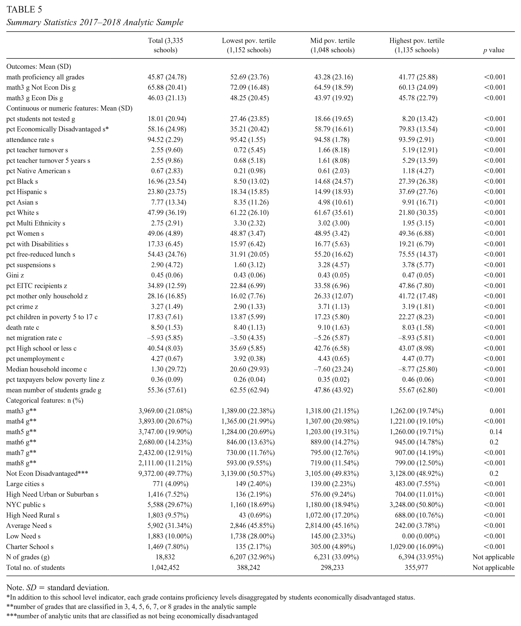
Note. SD = standard deviation.
In addition to this school level indicator, each grade contains proficiency levels disaggregated by students economically disadvantaged status.
number of grades that are classified in 3, 4, 5, 6, 7, or 8 grades in the analytic sample
number of analytic units that are classified as not being economically disadvantaged
Multilevel SAR Models for Posterior Means of Mathematical Proficiency Rates 2017–2018 Analytic Sample

Note. EITC = Earned Income Tax Credit; ELL = English language learner; MSAR = multilevel simultaneous autoregressive; NYC = New York City.
^ Comparison group is White students.
^^ Comparison is NYC schools.
^^^ The parameter space for these variables is to be (–1,1), and these tests were conducted independently from MSAR, as can be seen in the replication code.
p < .05. **p < .01. ***p < .0001.
Summary Statistics 2018–2019 Analytic Sample
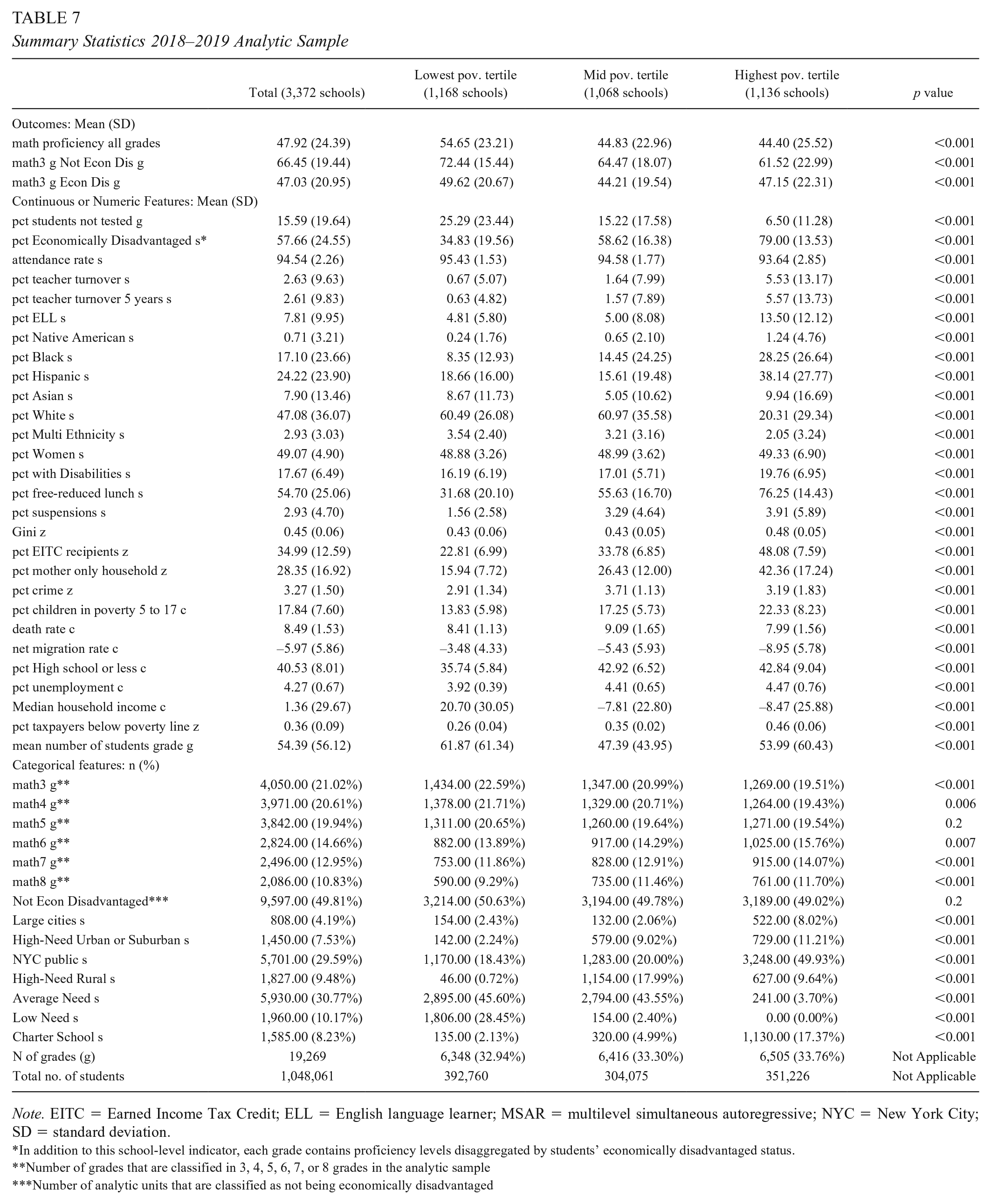
Note. EITC = Earned Income Tax Credit; ELL = English language learner; MSAR = multilevel simultaneous autoregressive; NYC = New York City; SD = standard deviation.
In addition to this school-level indicator, each grade contains proficiency levels disaggregated by students’ economically disadvantaged status.
Number of grades that are classified in 3, 4, 5, 6, 7, or 8 grades in the analytic sample
Number of analytic units that are classified as not being economically disadvantaged
Multilevel SAR Models for Posterior Means of Mathematical Proficiency Rates Analytic Sample 2018–2019

Note. EITC = Earned Income Tax Credit; ELL = English language learner; MSAR = multilevel simultaneous autoregressive; NYC = New York City; SAR = simultaneous autoregressive.
^ Comparison group is White students.
^^ Comparison is NYC schools.
^^^ The parameter space for these variables was to be (–1,1), and these tests were conducted independently from MSAR, as can be seen in the replication code.
p < .05. **p < .01. ***p < .0001.
Having said this, although all these results are included as robustness checks, my preferred specifications still remain those of the models that include both years of data. Conceptually and econometrically speaking, these time fixed-effects models allow the incorporation of time into the MSAR specification, an approach that the developers of MSAR recommended and implemented (see Dong et al., 2015). This methodological decision is important, for MSAR models are primarily cross-sectional, but I have demonstrated how researchers may include these temporal elements into their specification strategies. Having said that, in this case, it should be highlighted that the cross-sectional and time-effects models were consistent, but consistent with complex systems tenets that model life itself (see Gonzalez Canche, 2021), this may not necessarily be the case in models estimated with other data sources and that address different research questions.
Limitations: How Would Student Composition and Parents’ Wealth Affect the Findings?
The analytic sample accounted for all public schools at the state level, including charter schools, which are public schools yet also different from public schools (see Fischler, 2021). Although the models included all available data from public schools, it is possible that families who could afford to move, looking for better public schooling options, may have done so for the betterment of their students’ academic prospects or may have simply placed them in private schools. It could also be true that families with kids would have preemptively selected to live in “good public-school districts” rather than move to them, given the high costs associated with moving (Lindenfeld Hall, 2022; Pogol, 2019; Sahadi, 2015). Nonetheless, it is also possible that these parents may not have needed to move; instead, if they were located in high-poverty zones, they could have potentially enrolled their students at charter schools, which, as described above, tended to be overwhelmingly located in the highest poverty areas (with 71% of them located in such zones, as described in the findings section—see Table 3). Finally, another arguably less expensive strategy may have consisted of relying on private tutoring (online or in person) and/or on after-school programs.
If mobility is assumed to be the primarily driver that may ultimately influence students’ performance as a source of unobserved heterogeneity, note that moving, attending a private school, and/or buying a house in “good” public-school districts is expensive, which may not reflect the decisions that the vast majority of parents in our analytic samples may have made—as has been widely reported (Lindenfeld Hall, 2022; Pogol, 2019; Sahadi, 2015). Nonetheless, following the rationale of compositional changes based on parents’ decisions to move their students, given such parents’ socioeconomic standing, the worst-case scenario that may have translated into heightened compositional changes was supposed to affect grades and schools located in more affluent regions. This implies, then, that the set of models that should be “distrusted” the most are those measuring mathematical performance in the wealthiest neighborhoods in the analytic samples—after all, the types of students attending those areas would, in theory, have been coming from households that may have been able to afford to move into those areas and schools, precisely based on their known higher level of school quality. Alternatively, the mathematical performance in these wealthier zones may have been influenced by parents’ decisions to send their students to private schools, which means that the models would not have captured these students’ mathematical performance—that is, these wealthiest kids would likely not have been part of the analytic sample.
Despite these possibilities, the results of the models of students attending wealthier school districts are consistent with the results found among students attending schools located in less economically privileged neighborhoods. These models’ agreements alleviate concerns that student compositional changes may have resulted in misleading findings or grossly erroneous conclusions. Nonetheless, unfortunately, I do not have access to data that would have captured the specific movement of students from poor areas to enroll at schools located in wealthier zones (or movement from public non-charter to charter schools or participation in after-school programs or private tutoring). Indeed, I am not familiar with any available data set that is detailed enough to capture such a movement (or such parental strategies to improve their students’ mathematical ability). Having said this, although this movement analysis was not a goal in this study, it motivated me to account for net outmigration as part of the control indicators included in the models. Moreover, despite those idiosyncratic decisions made by families, I am confident that because moving and attending private school are expensive, the models shown in this study captured most of the experiences of typical students rather than those experiences of privileged families who were embarking in this strategic movement and school choice. As with any statistical model, outlier cases may be present, and the experiences of these atypical and privileged cases may surely have diverged from the overwhelming majority reflected in the analytic samples, which should not disqualify this paper or my inferences. Having said this, despite the fact that I tested and accounted for two different forms of spatial dependence present in the analytic samples, which, if left unmodeled, may have been sources of bias I am not claiming causality or absolute lack of bias. As a matter of fact, given the untestable set of assumptions required to claim causality, I strongly refrain from making causal claims in education and in social science research.
Before listing another limitation of the study, it should be noted that researchers interested in mapping and estimating the impact of this student mobility (and/or participation in private tutoring or after-school programs) could do so with individual-level panel data access. However, I do not have such data sources, despite having requested such access. Nonetheless, reliance on publicly available administrative data has allowed me to showcase how applied researchers may leverage these data to offer innovative and nuanced estimates of factors affecting mathematical proficiency that are fully reproducible; all data and code can be accessed at https://cutt.ly/N4zRstL.
Another limitation of this study is that although economic disadvantage encompasses a wide array of factors that may capture students’ economic challenges, and although students may experience more than one of these indicators, the NYSED data do not provide levels of economic disadvantage. From this view, rather than having a single dichotomic indicator, when possible, future studies should provide more nuanced measurements (perhaps categorical or even numeric) of the economic conditions that may influence students’ prospects of remaining mathematically proficient. As depicted in this study, even though the analyses and findings are informative in capturing performance gaps based on this binary indicator, to the extent that the geography of mathematical disopportunity is prevalent—that is, to the extent that students experience a concentration of these economic challenges at the individual, school, and geographical levels—their opportunities for upward mobility will surely decline.
Methodological Discussion and Implications: How Specific Should Nesting Structures Be When Not Relying on Multilevel Simultaneous Autoregressive to Address Residual Autocorrelation?
As discussed in the methods section, multilevel models are the standard to address nesting structures that may affect outcome variation over and above individual-level attributes. From this perspective, González Canché (2021, 2014, 2021, 2023b) and Wolf et al. (2021) demonstrated that when the nesting structure is specific enough, model residuals obtained from multilevel models (i.e., not spatial multilevel models) will successfully address outcome dependence that may then result in spatial outcome dependence or autocorrelation (see González Canché, 2023b). However, as these nesting structures become less specific (i.e., moving from nesting at the classroom, to nesting at the school, to nesting at the school district, to nesting at the county or state level), spatial outcome dependence or autocorrelation may result in the presence of residual dependence—that is, in not identically and independently distributed (iid) residuals.
With this understanding, one of the study’s reviewers encouraged me to demonstrate whether these patterns were realized when analyzing the public administrative data employed in this study, with an emphasis on comparing not only whether model residuals became iid but also on how model coefficients differed or remained congruent with the model coefficients found with MSAR. Table 9 addresses this recommendation, including the aggregate model shown in Table 4 as well as two nonspatial multilevel models: one nesting classrooms at the school level and another where the nesting structure was conducted at the ZCTA level, hence matching the two levels used in every MSAR specification employed in this study.
Comparison Coefficient Magnitudes and Residual Dependence Issue of MSAR and Multilevel-Alone Models With Divergent Nesting Structures

Note. EITC = Earned Income Tax Credit; ELL = English language learner; MSAR = multilevel simultaneous autoregressive; NYC = New York City; ZCTA = zip code tabulated area.
^ Comparison group is White students.
^^ Comparison is NYC schools.
^^^ The parameter space for these variables was to be (–1,1), and these tests were conducted independently from MSAR, as can be seen in the replication code.
This is the aggregated model shown in Table 4. Replication code starts on line 394 in the file called “Replication_data_code_math_2018-2019.R” located at https://cutt.ly/N4zRstL.
p < .05. **p < .01. ***p < .0001.
Table 9 shows that if the nesting of grade levels was identified or operationalized at the school level, residual dependence became iid. On the other hand, when this nesting structure was specified at the ZCTA level, the models once again suffered from residual dependence—that is, the resulting model residuals were not iid. These findings and patterns were then congruent with past research (González Canché, 2014, 2021, 2023b; Wolf et al., 2021): When the nesting structures were less specific, model residuals would remain an issue in nonspatial multilevel models.
With respect to model coefficients, although the less specific nesting structure suffered from residual dependence (nested ZCTA model in Table 9—see also Gonzalez Canche, 2014), some of its coefficients were closer in magnitude to the coefficients found via MSAR. For example, gaps between Grades 3 and 8 math had a magnitude of 20.87 and 20.83 percentage points in the MSAR and the nested ZCTA models, respectively, but this magnitude in the Nested School model indicated a gap between students in Grades 3 and 8 of only 17.31 percentage points. Other coefficients, however, resulted in notable differences. For example, the percentage of single-mother households was statistically significant in both multilevel models, but not in the MSAR specification, which may have been a function of the former not incorporating any spatial information as part of the model estimation. From this perspective, when considering that MSAR models were capable of (a) accounting for two forms of nesting structures, (b) accounting for fixed effects via the matrix ∆ that captured schools’ ascription to ZCTAs, and (c) rendering residuals that were iid, I consider the MSAR estimates to have been more robust to multiple sources of bias.
Based on this brief discussion, multilevel-alone models (i.e., not spatial multilevel models) may have either suffered from residual dependence (like the ZCTA nesting structure model) or rendered coefficients that were arguably downwardly biased (i.e., like the school nesting structure model). Having said this, it should be noted that despite the statistical benefits associated with MSAR, these models remained cumbersome to be operationalized and executed. This complexity was based on the need to create three matrices of influence (
Discussion: The Geography of Mathematical (Dis)Advantage
The study’s purpose was to offer nuanced estimates of proficiency rates in mathematics across grades while simultaneously considering test-takers’ own economic standing and schools’ contextual and place-based observed poverty levels. The results consistently indicate that proficiency rates decreased as cohorts of students advanced through elementary and middle schools, with the highest decreases observed in Grade 8. Note that although these drops in proficiency rates were congruent with the gaps reported by the NAEP (2020), this study’s estimates show a grimmer picture and also provide evidence of a geography of mathematical disopportunity, wherein the interaction of economic disadvantage and place-based poverty results in the lowest change of remaining mathematical proficiency across grades, but with interesting and more nuanced patterns. For example, Grade 8 students who were economically disadvantaged and attended schools located in the highest poverty zones realized the lowest gaps among all students, with changes in proficiency rates of –15.31% with respect to their Grade 3 test-taker counterparts.
These findings convey mixed results. On the one hand, students who arguably were the most vulnerable (Pearman, 2019) had the lowest gaps with respect to their Grade 3 peers. On the other hand, these findings are not positive when observing that the mean mathematical proficiency rates of Grade 3 students attending schools in the highest poverty zones (see Table 3) were the second lowest among all Grade 3 students (46.62%, SD = 22.47). When considering these starting points, the 26.38 percentage-point decrease in mathematical proficiency (standard error 0.912) observed among non–economically disadvantaged Grade 8 students attending schools in the lowest poverty zones (see Table 4), when compared to the 15.31 percentage-point decrease realized by Grade 8 students in high-poverty schools (standard error 0.768), implied that the former test-takers had proficiency rates that still remained 14.92 percentage points higher than those of economically disadvantaged Grade 8 students attending schools located in high-poverty zones. For the sake of clarity, let us elaborate on this 14.92 percentage-point gap among Grade 8 test-takers. Note that non–economically disadvantaged Grade 3 test-takers had mathematical proficiency levels of 72.27%, whereas economically disadvantaged Grade 3 test-takers reached mathematical proficiency levels of 46.62%. Considering this, the 26.38 percentage-point decrease observed among Grade 8 test-takers attending schools located in low-poverty areas led to a performance of 46.23% for these non–economically disadvantaged students (or 72.27 – 26.038 = 46.232). In the case of their economically disadvantaged peers attending schools located in high-poverty areas, when considering that the Grade 3 performance was 46.62%, the lower magnitude observed in the Grade 8 coefficient (–15.31%, as shown in Table 4) indicates that these Grade 8 students reached mathematical performance rates of 31.31% (or 46.62 – 15.307 = 31.313). Taking the differences of these two differences yields a performance gap among Grade 8 students of 14.92 percentage points (or 46.23 – 31.31). That is, although the magnitude of the coefficients shown in Table 4 seemed to be worse for non–economically disadvantaged Grade 8 test-takers attending schools located in low-poverty zones, the ultimate mathematical performance of their economically disadvantaged Grade 8 peers attending schools located in high-poverty areas was still much more dire.
In sum, although proficiency gaps between economically disadvantaged students in Grades 3 and 8 attending schools located in high-poverty zones were the smallest across all groups, performance gaps between economically disadvantaged and non–economically disadvantaged Grade 8 students favored the latter. In going back to the hypothetical relationships, these findings partially corroborated the hypothesis that “economically disadvantaged students would likely experience greater losses in mathematical proficiency levels compared to their non–economically disadvantaged peers.” As just depicted, although these losses were greater in magnitude for non–economically disadvantaged Grade 8 test-takers, the end result was the same: Economically disadvantaged students remained less proficient than their non–economically disadvantaged peers.
The consistent finding across model specifications between opting out from testing and mathematical proficiency reflected no evidence of purposeful exclusion of students from testing. That is, had these results reflected a positive association between percentage of students who were not tested and performance in math, this could have been perceived as students who may not have been identified/self-identified as nonproficient deciding not to participate or as school administrators preferring that they not participate in this standardized testing process. Also aligned with the notion of the geography of mathematical disopportunity, overall, schools located in the lowest poverty zones (see Table 3) had many advantages: They had the lowest turnover rates, lowest suspension levels, lowest percentage of students classified as economically disadvantaged, and the highest median income at the county level, which may have translated into higher levels of funding based on property taxes. Their students also performed the best.
Considering the positive spillover effects of mathematical proficiency, programs and policies should strive for all schools, but particularly the most socioeconomically vulnerable schools and at younger ages, to increase or maintain their students’ proficiency rates. In this respect, note that participation in free and reduced-price lunch programs was consistently associated with increases in mathematical proficiency levels in these poorest areas; as indicated above, current national movements are pushing for the adoption of healthy school lunches at public and not-for-profit public schools. Recent in-person class interruptions due to COVID-19 highlighted that these programs often represented the main source of food for students living in the highest poverty zones. Accordingly, this study offers evidence to reinforce the positive impact that these programs may have in mathematical proficiency prospects, regardless of students’ economic health.
The comparison of NYC schools and charter schools reflected that proficiency rates in the latter were at least 8.7 percentage points higher in high-poverty areas for economically disadvantaged and non–economically disadvantaged students, with the highest gains observed among economically disadvantaged test-takers attending schools in high-poverty areas. Although charter schools are public schools, they are also different from public schools (Fischler, 2021). In this respect, it should be noted that non-charter public schools could potentially benefit from collaborating with or implementing programs similar to those implemented by their charter counterparts, particularly because 71% of these charter schools were located in the highest poverty areas and were succeeding at higher rates.
To close, because 80% of students attending the highest poverty level zones were also classified as economically disadvantaged, positive spillovers of mathematical proficiency indicate that actions geared toward increasing their mathematical competence may lead to increasing their performance in other academic areas (Duncan et al., 2007; Farran et al., 2006; Lerkkanen et al., 2005; Pagani et al., 2010). The intrinsic relationship between mathematics and STEM, along with the relevance of these fields in the present and future economies, suggests that to the extent that more students, particularly those from economically disadvantaged backgrounds, become and remain proficient in mathematics, their prospects of success in life will increase (González Canché, 2017). Mathematical proficiency is a worthwhile pursuit with equitizing, gap-closing implications.
In terms of areas for future research, researchers may build from the concepts and data set provided in this study to assess the impact of the COVID-19 pandemic on mathematical proficiency for economically disadvantaged and non–economically disadvantaged students. This endeavor is worthwhile, for the NAEP (2022) reported that although mathematical proficiency rates nationwide between students in Grades 4 and 8 had widened by 10 percentage points, favoring the former, in New York State, there was no gap, with a 28% proficiency score in 2022 in Grades 4 and 8. However, these depictions may be misleading by failing to account for test-takers’ economically disadvantaged statuses along with the poverty rates and locations of their schools. Accordingly, future studies may leverage MSAR difference-in-differences by incorporating data on performance observed after the pandemic and compare these performance rates between economically disadvantaged and non–economically disadvantaged test-takers. In addition to being beyond the scope of this study, due to data availability constraints—there has been no post-pandemic data release by the NYSED—I am unable to offer these estimates but such analyses can be implemented following the code provided with this study. Finally, considering that charter students in high-poverty areas are doing better than their district peers, future research may study whether certain families in high-poverty areas are seeking better educational alternatives for their children and document who these families are to more clearly explain the mechanism behind this outstanding performance in the highest poverty zones.
Footnotes
Acknowledgements
I am grateful for the research support and conceptual and methodological discussions provided by Chelsea Zhang (PhD candidate and master’s in statistics candidate at the University of Pennsylvania; email:
Declaration of Conflicting Interests
The author declared no potential conflicts of interest with respect to the research, authorship, and/or publication of this article.
Funding
The author disclosed receipt of the following financial support for the research, authorship, and/or publication of this article: This study was funded by grants offered by the Spencer Foundation and the National Academy of Education Postdoctoral Fellowship as well as by a grant on education data analytics sponsored by the National Science of Education.
1.
Based on the New York State Education Department (NYSED, 2020a), students scoring 3 or 4 in a 1–4 Common Core Learning Standardized test administered at public elementary and middle schools in the state of New York were considered proficient in mathematics.
2.
Students classified as “economically disadvantaged” participate in assistance programs, such as free or reduced-price lunch, Social Security Insurance, food stamps, foster care, refugee assistance, EITC, Home Energy Assistance Program, Safety Net Assistance, Bureau of Indian Affairs, or Family Assistance: Temporary Assistance for Needy Families (NYSED, 2020a).
3.
Please note that lunch eligibility as a proxy for poverty measure is becoming less useful, as there has been a recent trend in district-level participation in the national lunch program (see National School Lunch Program by the U.S. Department of Agriculture at https://www.fns.usda.gov/nslp). I am thankful for this comment, which was raised by one of this study’s reviewers. However, the summary statistics in the analytic samples still showed a high degree of variation at the aggregated levels and when disaggregating the analytic samples by poverty levels of the zones where schools were located. Specifically, these disaggregated estimates ranged from 31.76% in the least poor areas to 75.93% in the highest poverty zones. These variation levels, along with the identification of this indicator as a relevant feature via Boruta (see ![]() ), as described in the methods section, justified its inclusion in the models.
), as described in the methods section, justified its inclusion in the models.
4.
This estimate was obtained as the ratio of taxpayers in a given zip code with adjusted income levels up to $25,000 over the total number of taxpayers in that same zip code. Considering that the state of New York indicated that the poverty line was $32,402 as of 2016 (Chatterjee et al., 2019), inhabitants with incomes up to $25,000 were considered to be at least $7,500 below this poverty line.
5.
Hence, participation in assistance programs, such as free or reduced-price lunch, Social Security Insurance, food stamps, foster care, refugee assistance, EITC, Home Energy Assistance Program, Safety Net Assistance, Bureau of Indian Affairs, or Family Assistance: Temporary Assistance for Needy Families (NYSED, 2020a).
8.
The NYSED counted the number of students per grade who took these Common Core Learning Standardized tests.
9.
10.
Including students with intellectual disability, hearing impairment, speech or language impairment, visual impairment, serious emotional disturbance, orthopedic impairment, autism, traumatic brain injury, developmental delay, other health impairment, specific learning disability, deaf-blindness, or multiple disabilities and who, by reason thereof, receive special education and related services.
11.
Higher level covariates captured at the county level could be added, but the main nesting structure was zip code. Spatial dependence at the county level indicated no spatial clustering, relying on Moran’s I, discussed below.
12.
To test for sensitivity of this 1.5-kilometer specification, the models were replicated with matrices W with distance thresholds of 2 and 2.5 kilometers rendering similar estimates. Another specification relied on a 0.6-mile threshold, as discussed by Chetty et al. (2020), who did not rely on matrices of influence, as in the case of Dong et al. (2015). Similarly, no differences in the estimates were found (because this specification represented a distance of .33 mile, because 1.5 kilometers = 0.93 mile), accordingly, the findings were assumed to not be sensitive to the variations discussed herein. All these specifications can be tested with the replication code provided at ![]() .
.
13.
The replication code identified g→s,z, relying on network principles by creating a composite key identifier of grades in schools that then were ascribed to ZCTAs to extract the block diagonal design matrix Δ.
14.
County-level indicators could be identified and would remain the same across zip codes that were located in a given county.
15.
16.
This feature selection was implemented with the Boruta package in R (see Kursa & Rudnicki, 2010).
17.
Robustness checks conducted with data disaggregated for the 2017–2018 and 2018–2019 academic years corroborated the relevance of all these indicators. These HTML Boruta figures may be accessed at https://cutt.ly/l4DSvLT and at ![]() for the 2017–2018 and 2018–2019 academic years, respectively.
for the 2017–2018 and 2018–2019 academic years, respectively.
18.
Highest: 66% lived below poverty levels. Lowest: 33% lived below poverty levels.
20.
Minimal or low-code tools ascribe to data science democratizing efforts by removing vast amounts of statistical and computer programming proficiency requirements (or barriers) to apply sophisticated and rigorous state-of-the-art analytic and data interactive data visualization techniques (Gonzalez Canche, 2023b).
Author
MANUEL S. GONZÁLEZ CANCHÉ is an associate professor at the University of Pennsylvania, 208 S. 37th St., Room 307, Philadelphia, PA 19104; email: ![]() .
.