Sage Journals: Discover world-class research

Abstract

Colleges have increasingly turned to predictive analytics to target at-risk students for additional support. Most of the predictive analytic applications in higher education are proprietary, with private companies offering little transparency about their underlying models. We address this lack of transparency by systematically comparing two important dimensions: (1) different approaches to sample and variable construction and how these affect model accuracy and (2) how the selection of predictive modeling approaches, ranging from methods many institutional researchers would be familiar with to more complex machine learning methods, affects model performance and the stability of predicted scores. The relative ranking of students’ predicted probability of completing college varies substantially across modeling approaches. While we observe substantial gains in performance from models trained on a sample structured to represent the typical enrollment spells of students and with a robust set of predictors, we observe similar performance between the simplest and the most complex models.

Keywords

predictive analytics college success data science community colleges

Predictive analytics have become increasingly common in the education sector. Colleges and universities use predictive analytics for various purposes, ranging from identifying students who might default on their loans to targeting alumni who are likely to give generously to the institution (Ekowo & Palmer, 2016). The most common use of predictive analytics, however, is to identify students at risk of failing courses or dropping out (Alamuddin et al., 2019; Milliron et al., 2014; Plak et al., 2019), and to direct various student success strategies (e.g., intrusive advising, additional financial aid) to these students. Numerous contextual factors have motivated institutions to turn toward predictive analytics. While enrollment rates have increased steadily over the past decade and socioeconomic inequalities in college participation have narrowed (U.S. Department of Education, 2019), completion rates remain relatively stagnant and socioeconomic disparities persist and have widened over time (Bailey & Dynarski, 2011; Chetty et al., 2020). Students are borrowing a record amount of money to fund their postsecondary education—total student debt now exceeds $1 trillion—with default rates highest among students who drop out before finishing their degree (Bastrikin, 2020; Looney & Yannelis, 2015). In light of these trends, state and federal policy makers have put increasing pressure on institutions to increase completion rates.

Despite this increased pressure, at broad-access institutions attended by most undergraduates, the level of resources available to invest in completion strategies has declined considerably over time as states have reduced their appropriations to public higher education (Deming & Walters, 2017; Ma et al., 2017). The use of predictive analytics in higher education has the potential to increase efficiency in how scarce resources are allocated by targeting students who may benefit most from additional intervention. Adoption of predictive analytics strategies has been broad and rapid; a third of all institutions have invested in predictive analytics and collectively spend hundreds of millions of dollars on technology that utilizes predictive analytics (Barshay & Aslanian, 2019).

For efficiency gains to be realized from predictive analytics, though, predictions from underlying models must be accurate, stable, and fair. However, in most cases, researchers and college administrators have little to no ability to evaluate predictive analytics software on these dimensions, as most predictive analytics products used in higher education are proprietary and operated by private agencies. This lack of transparency creates multiple risks for institutions and students. Models may vary substantially in the accuracy with which they identify at-risk students, which can lead to inefficient and ineffective investment of institutional resources. Furthermore, biased models can lead institutions to intervene disproportionately with students from underrepresented backgrounds and may reinforce existing psychological barriers that students encounter, including feelings of social isolation and anxiety (Walton & Cohen, 2011).

In this article, we address the lack of transparency in predictive analytics in higher education by systematically comparing two important dimensions of predictive modeling. First, we compare different approaches to sample and variable construction and how these affect model accuracy. We focus in particular on how two analytic decisions affect model performance: (1) random truncation of a current cohort sample to align to the enrollment length distribution of historic cohorts and (2) the inclusion of term-specific and more complexly specified variables (e.g., a variable measuring the trend in students’ GPA over time). Second, we investigate how the choice of modeling approach, ranging from methods many institutional researchers would be familiar with, such as ordinary least squares (OLS) regression and survival analysis, to more complex approaches like tree-based classification algorithms and neural networks, affects model performance and the stability of student predicted scores (i.e., “risk rankings”).

We examine these features of predictive modeling in the context of the Virginia Community College System (VCCS), which consists of 23 community colleges in the Commonwealth of Virginia. We have access to detailed student records for all students who attended a VCCS college from 2000 to the present. Community colleges serve numerous functions, including targeted skill development, broader workforce readiness, terminal degree production, and preparation to transfer to a 4-year institution. Each of these functions have different potential measures of success. In this article, we focus in particular on the outcome of whether students graduate with a college-level credential within 6 years of initial entry to systematically compare predictive modeling strategies.

Our analysis yields several primary conclusions. First, while models are very consistent in whether they predict whether a given student graduates, they vary in how they rank a given student’s predicted probability of graduating. For instance, among students that the OLS model ranks in the bottom decile of the probability of completing college, only 60% are also ranked in the bottom decile according to the XGBoost approach. This lack of consistency in student ranking holds across the distribution of risk. This result suggests that the notion of relative “risk” is not stable and can be quite sensitive to the modeling strategy used. For institutions that use predictive modeling to intervene with a targeted subset of students, such as students at greatest risk of dropout, different models are likely to identify different students for intervention.

Second, predictive models that leverage randomly truncated samples, term-specific predictors, and more complexly specified variables have higher performance than models trained on samples without truncation or with basic variables (e.g., cumulative credits completed) that may be more readily available to higher education administrators and institutional researchers. This suggests there are gains to complexity in sample and variable construction, whether institutions pursue that work internally or through an external vendor. Finally, in terms of modeling approach, we do not observe substantial increases in accuracy from more complex models. All models we compare have high levels of accuracy in predicting whether a student will graduate or not.

We contribute to the evidence base on the efficacy of predictive analytics in higher education in this article in several ways. Ours is the first article, of which we are aware, that systematically evaluates and compares the performance of different sample and variable construction approaches and modeling strategies in an applied setting. In doing so, we bring transparency to a practice that is increasingly common but frequently opaque in higher education. Our findings also elucidate the trade-offs to common modeling decisions and the contexts in which the expected returns to sophisticated machine learning methods (over and above conventional regression-based models) are largest. Finally, we discuss important questions around the ethics, cost, and efficacy of using predictive analytics that higher education administrators and researchers may want to consider in determining their approach to predicting student success.

Conceptual Model

To develop a conceptual model of how administrators at broad-access institutions use predictive analytics, we draw on several reports that collectively provide case studies of how dozens of institutions have incorporated predictive analytics into their practice (Association of Public & Land-Grant Universities, 2016; Burke et al., 2017; Ekowo & Palmer, 2016; Klempin et al., 2018; Paterson, 2019; Stark, 2015; Treaster, 2017). In this review, we observe two broad commonalties in predictive analytics usage. First, nearly all institutions’ use of predictive analytics is in response to two interwoven contextual factors: (1) increasing pressure on institutions to increase success rates, including shifts in state public financing for higher education toward outcomes-based funding allocations and (2) declining overall state appropriations toward public higher education, which result in institutions having fewer resources to allocate toward college success strategies and interventions. These combined factors increase pressure on institutions to target scarce resources as efficiently as possible to achieve meaningful improvements in success outcomes. Second, while most institutions use data to inform broad institutional practice, the predictive analytics applications are primarily geared toward targeting individual student outreach, primarily through faculty or advisor intervention.

Institutions apply predictive analytics across the life cycle of students’ engagement with the institution. For instance, predictive analytics have become increasingly commonplace in enrollment management and financial aid packaging as broad-access institutions have become increasingly reliant over time on tuition as a primary source of revenue. Institutions like Wichita State University use models to target recruitment and marketing investments to students most likely to apply and matriculate, enroll, and succeed at the institution (Ekowo & Palmer, 2016). Institutions like Jacksonville State University and University of Texas–Austin use models to inform aid allocations, respectively, directing scholarships to students who are predicted to stay enrolled at the institution (rather than transfer elsewhere) or to students who are predicted to drop out absent additional financial support (Ekowo & Palmer, 2016; Paterson, 2019).

Institutions also use predictive analytics to identify courses in which academic performance is predictive of later success at the institution, and to target interventions to students who are predicted to struggle in those courses. For instance, the University of Arizona learned from a predictive model that students who earn a C in introduction English composition have a lower probability of graduating, and they allocated additional academic supports to such students (Treaster, 2017).

By far the most common use of predicted analytics reported in these case studies is to identify students at risk of dropping out before completing their degree. Georgia State University has received substantial attention for its use of predictive analytics to identify students who were struggling academically and to provide them with additional support. Like many other institutions that use predictive analytics to identify students at risk of withdrawal prior to completion, Georgia State partnered with a private company (EAB) to develop an algorithm using student-level administrative data from numerous historic cohorts. Other institutions like Temple University developed their own predictive analytics models and “early alert” systems to identify at-risk students. Across the institutions featured in the case studies we reviewed, most leveraged the “early alerts” generated by predictive models to either trigger proactive outreach from academic advisors to students or to encourage faculty to reach out to students in their classes who were struggling to succeed (Ekowo & Palmer, 2016). At some institutions, like the University of North Carolina–Greensboro, administrators group students into deciles of predicted risk of withdrawal and target more intensive interventions to students with the highest risk ratings (Klempin et al., 2018).

These common uses of predictive analytics by administrators at broad-access institutions rest on the assumption that the underlying prediction models—whether for enrollment management or to target student success interventions—are producing student-level risk predictions that are accurate, stable, and fair. In the remainder of the article, we investigate the extent to which these assumptions hold across predictive modeling approaches.

Empirical Strategy

Data

The data for this study come from VCCS system-wide administrative records over the summer 2007 through spring 2019 academic terms. These records include detailed information about each term in which a student enrolled, including their program of study, courses taken, grades earned, credits accumulated, financial aid received, and degrees earned. The records also include basic demographic information, including gender, race, and parental education. Finally, we observe all credentials awarded by VCCS colleges beginning in 2007. In addition to VCCS administrative records, we also have access to National Student Clearinghouse graduation and enrollment records. National Student Clearinghouse data allow us to observe all enrollment periods and postsecondary credentials earned at non-VCCS institutions from 2004 onward.

Outcome Variable Definition

We focus on predicting the probability a student completes any college-level credential within 6 years. For simplicity, we refer to our outcome as “graduation” throughout the article. Based on this outcome definition, 34.1%% of students in our sample graduated. We choose to focus on the outcome of graduation rather than dropout because dropout is more ambiguous and difficult to define, particularly in the community college context. For instance, if a student leaves for a few semesters, it is unclear whether they “stop out” and plan to return to college at a later date or have dropped out with no plans to return. Within our sample, 37.7% of students leave VCCS for at least one nonsummer term and later return to higher education (either to VCCS or to a non-VCCS institution); 23.3% of students leave for at least one full year and later return to higher education.

While all VCCS credentials are designed to be completed in 2 years or less if the student is enrolled full-time, prior research has shown that only 16% of certificate earners and only 5% of associate degree earners graduate within 2 years (Complete College America, 2014). We focus on graduation within 6 years because we consider credential completion from both VCCS and non-VCCS institutions, some of which are 4-year institutions students transfer to after their enrollment at VCCS.¹

Sample Construction

Our sample consists of students who enrolled at a VCCS college as a degree-seeking, nondual enrollment student for at least one term, with an initial enrollment term between summer 2007 and summer 2012 (the last cohort for whom we can observe 6 years of graduation outcomes). We provide additional details on our sample definitions in the online Supplemental Appendix 1.

For each student in our sample, we observe their information for the entire 6-year window after their initial enrollment term. While in all of our models we use the full 6 years of data to construct the outcome measure, we test two different approaches to constructing model predictors. First, using data from students initially enrolled between summer 2007 and summer 2012, we construct a sample using all information from initial enrollment through the term when the student earned their first college-level credential, or the end of the 6-year window, whichever comes first. The primary concern with this approach to predictor construction is that models fitted using all available data for historical cohorts of students may not be generalizable to currently enrolled students, whose enrollment spells do not extend to the full 6 years or to credential attainment. Therefore, in our second approach, also using data from students initially enrolled between summer 2007 and summer 2012, we construct a historical sample of students using a random truncation procedure that resembles the distribution of enrollment lengths for currently enrolled students.

The first two columns of Table 1 show the distribution of the number of terms since initial VCCS enrollment for students enrolled in fall 2012 (the most recent fall term in our sample). In the first row, we see that 33% of students enrolled at a VCCS institution in fall 2012 first enrolled in that term, and their enrollment length is therefore equal to one term. In our second approach to predictor construction, we randomly truncate the data in the full sample to resemble the distribution of enrollment lengths among fall 2012 enrollees. For example, we randomly assign 33% of students from the training and validation samples to have an enrollment length of one— in other words, for those students, we only use their first term of data to construct their model predictors, regardless of how long they were actually enrolled at VCCS. Columns 3 and 4 of Table 1 show the full distribution of enrollment lengths in the truncated training and validation samples, which are described below. The modal length of enrollment is one term, but there is substantial variation across students. For example, 17% of students have an enrollment length of four terms. We discuss in more detail the motivation and steps for our approach to sample truncation in the online Supplemental Appendix 1.

Table 1

Distribution of Enrollment Length for Fall 2012 Enrollees and Truncated Training and Validation Samples

Enrollment length	Fall 2012 enrollees	Truncated training sample	Truncated validation sample
(1)	(2)	(3)	(4)
1	0.333	0.333	0.3331
2	0.0433	0.0433	0.0432
3	0.0757	0.0756	0.0756
4	0.1696	0.1696	0.1696
5	0.0263	0.0264	0.0264
6	0.0456	0.0456	0.0456
7	0.0973	0.0973	0.0973
8	0.0152	0.0152	0.0152
9	0.0298	0.0298	0.0298
10	0.0591	0.0591	0.0591
11	0.01	0.01	0.01
12	0.0177	0.0177	0.0177
13	0.034	0.034	0.034
14	0.006	0.006	0.006
15	0.0107	0.0107	0.0107
16	0.0225	0.0225	0.0225
17	0.0042	0.0042	0.0042
N	115,413	298,139	33,115

Note. Enrollment length refers to the number of terms since initial Virginia Community College System enrollment, including Fall, Spring, and Summer terms, and including terms in which the student was not enrolled. The truncated training and validation samples include data up through each student’s randomly assigned enrollment length in order to construct predictors. See text for more details.

Our resulting analytic sample consists of n = 331,254 students, which we randomly divide into training (90%) and validation sets (10%).² The training set is used to construct and fine-tune predictive models, while the validation set is held out throughout the model construction and tuning process and is used to evaluate the performance of the final prediction model. This division is standard practice in predictive modeling work to ensure that the model is evaluated on “unseen” data and therefore free of bias due to model overfitting.³ We further discuss the summary statistics of the full analytic sample in the online Supplemental Appendix 1.

Predictor Construction

In addition to exploring how different sample constructions affect model performance, we investigate how the incorporation of predictors with differing degrees of complexity affects model performance. We first test models that use simple, non-term-specific predictors most readily available to higher education administrators and researchers. These predictors include demographic information (e.g., race/ethnicity, parental education) along with a set of cumulative measures up to a student’s last observed term (overall or within the randomly truncated observation window), such as cumulative GPA and the share of all attempted courses the student completed. Second, we examine how model performance changes with the inclusion of additional non-term-specific predictors that are more complex to construct, such as the number of terms and quality of non-VCCS institutions a student attended before VCCS, and the standard deviation of a students’ term GPA in all previous enrolled terms. Third, we investigate how model performance is affected by the further inclusion of simple term-specific predictors, such as term-specific GPA, credits attempted, and the share of attempted credits earned. Finally, we include more complexly specified term-specific predictors, including academic and financial aid information such as term-specific credits withdrawn, 200-level credits attempted, the amount of financial aid received, and enrollment intensity at non-VCCS institutions. Online Supplemental Appendix 2 provides a full list of the predictors we test, organized by the sequence in which we test their inclusion in the prediction models.

Predictive Models

We use six different but commonly used estimation strategies in the social and computational sciences to predict the probability of credential attainment within 6 years (Attewell & Monaghan, 2015; Hand et al., 2001; Herzog, 2006): OLS, logistic regression, Cox proportional hazard (CPH) survival analysis, random forest, gradient boosted machines (XGBoost), and recurrent neural networks (RNN).

OLS, logistic regression, and CPH are models commonly used by researchers in all areas to perform predictive modeling tasks, due to their ease of implementation and interpretation. We include OLS and logistic regression due to user familiarity, fast run times, and high degree of interpretability of output.⁴

CPH is one the most commonly used methods of survival analysis in the social sciences when the goal is to predict not only whether but also when the likelihood of an event will occur.⁵ Although our goal in this article is to predict whether students will complete college at any point within a 6-year window and not the timing of completion within that window, we include CPH among the estimation strategies we compare because survival analysis methods may be familiar to institutional researchers who are considering using predictive analytics in higher education. As we discuss in further detail in the online Supplemental Appendix 3, two limitations should be considered when comparing the performance of CPH models to the performance of the other estimation strategies we employ. First, we exclude time-varying predictors from CPH models because the assumptions required for their inclusion (i.e., for each currently enrolled student, we must impute the values of all time-varying predictors in all future, unobserved terms over the 6-year window) are extremely strong. Nevertheless, it remains possible that model performance would improve with the inclusion of time-varying predictors. Second, although survival analysis models can address complications associated with time-censored data using alternative approaches to random sample truncation (e.g., inclusion of model parameters to account for unobserved heterogeneity), we only estimate the CPH model on the randomly truncated sample. We do so because, as the results in Table 1 show, applying a model trained on a nontruncated sample of previously enrolled students to generate out-of-sample predictions for currently enrolled students raises questions of model generalizability that alternative approaches may not address. In addition, using the randomly truncated training sample allows for more interpretable intermodel comparisons since our primary predictions from all other models are derived using the randomly truncated sample. Compared with OLS, logistic regression, and survival analysis, tree-based methods (random forest and XGBoost) and neural network models (RNN) are less commonly used in the field of education, in part because they are more complicated to implement.⁶ However, they generally exhibit superior predictive performance because they more easily allow for capturing nonlinear and interactive relationships between the outcome and predictors. The basic building blocks of tree-based methods are decision trees, which flexibly identify patterns (sometimes quite complex) between the outcome of interest and the predictors (Breiman et al., 1984; James et al., 2013). However, because decision trees are highly sensitive to the sample and set of predictors included in building the tree, individual decision trees typically are not generalizable (i.e., they do not perform well on unseen data). We address this limitation through the use of two tree-based ensemble models, random forest and XGBoost. We describe additional detail and considerations for the implementation of tree-based methods in the online Supplemental Appendix 3.

Neural networks are a class of predictive modeling techniques whose model architecture resembles the network of biological neurons. Neural networks make predictions using highly complex patterns between inputs and the outcome of interest using a sequential “layering” process. RNN are a special type of neural network that sequentially transmit information of time-dependent inputs through “recurrent” layers. Although RNN models can exhibit strong performance in complicated, sequence-dependent prediction tasks, they are especially complex and computationally demanding.

As we show below, the most accurate models use the full set of predictors described above (i.e., both basic and complex non-term- and term-specific predictors). The base models we test thus include the full set of predictors.⁷ For the OLS, logit, random forest, and XGBoost models, we also rank order the predictors based on their “importance”—that is, their explanatory power in predicting the probability of graduation within 6 years. We provide additional details about the predictor importance measures in the online Supplemental Appendix 3.

Model Comparison and Evaluation Methods

Our aim is to compare the accuracy and stability of the predictions generated from the six different prediction methods that we tested. To make these comparisons, we calculate five evaluation statistics on the validation sample for each model⁸:

C-statistic: a measure of “goodness of fit” of predictive models. Specifically, the c-statistic is equal to the probability that a randomly selected student who actually graduated has a higher predicted score than a randomly selected student who did not graduate.

Precision: a measure capturing how often a model’s positive prediction is correct. Specifically, the precision value is equal to the share of students the model classifies as graduates (predicted positives) who actually graduated (true positives), that is, $Actual graduates / Predicted graduates$ .

Recall: a measure capturing a model’s ability to correctly classify actual graduates as predicted graduates. Specifically, the recall value is equal to the share of actual graduates that the model correctly predicts will graduate, that is, $Predicted graduates / Actual graduates$ .

F1-score: a measure that accounts for the inherent trade-off between precision and recall as the prediction score threshold used to distinguish students classified as graduates versus nongraduates changes. Mathematically, the F1-score is equal to the harmonic mean of precision and recall (i.e., $2 * [(Precision * Recall) / (Precision + Recall)]$ ) and ranges from 0 to 1, with higher values denoting stronger model performance.

Rank order of predicted scores: Models may have very similar overall performance but generate inconsistent predictions for a given student, especially in terms of relative risk. For every combination of model pairs, we therefore calculate the magnitude of change across each student’s predicted score percentile in Models A and B. We then report summary statistics of within-student distributional changes in predictions across models.

Results

Full Versus Truncated Sample

We first compare the model performance of the full training sample to the model performance using the truncated training sample for models that only include simple non-term-specific predictors as well as models that include both simple and complex non-term-specific predictors.⁹ We present the results in Figure 1. For all models, we observe an increase of 0.03 to 0.09 in c-statistic values for the truncated training sample compared with the nontruncated training sample. Furthermore, the performance of random forest and XGBoost models on the nontruncated training sample using only simple non-term-specific predictors (Panel A) are comparable to the performance of OLS and logit models on the truncated training sample using all the non-term-specific predictors (Panel B). This suggests that it is possible to achieve strong model performance with the simplest approaches to sample and variable construction; however, doing so requires more sophisticated modeling approaches.¹⁰ We also report the c-statistic values for comparing model performance of different sample construction methods in columns 1 to 4 of the online Supplemental Appendix Table A1.

Figure 1.

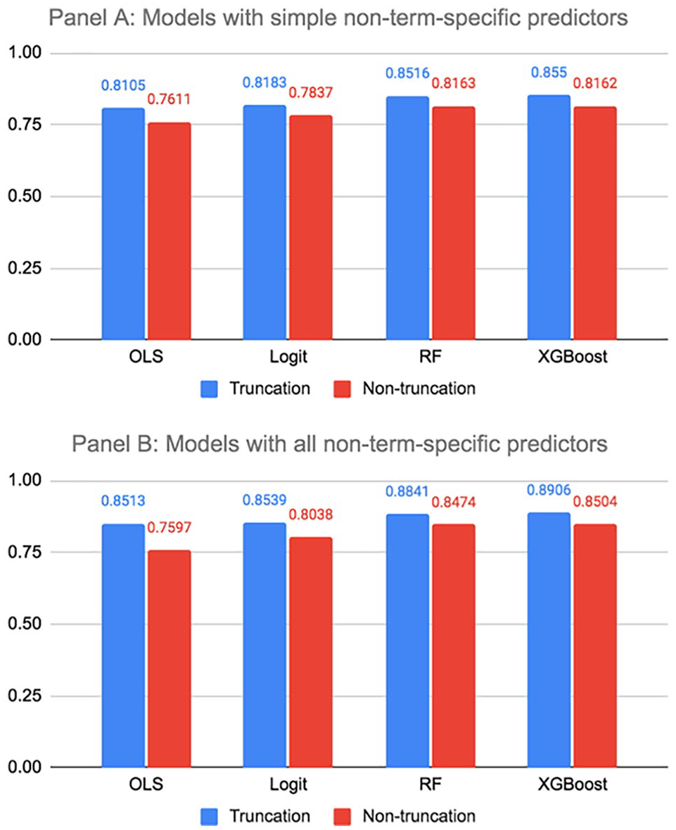
Model performance (c-statistic) under different sample construction methods.

Complexity of Variable Construction

Having demonstrated the improvement in model performance from using truncated samples that more closely resemble current enrolled students, we now turn to assessing the impact of model performance when simple versus more complexly specified predictors are used to predict graduation. Figure 2 shows that models that only include 14 basic non-term-specific predictors produce relatively informative and reliable predictions. OLS and logit models generate c-statistics between 0.81 and 0.82; the CPH model produces a c-statistic of 0.84, and random forest and XGBoost models yield c-statistics between 0.85 and 0.86. However, we observe that adding more complexly specified non-term-specific predictors to the models, for a total of 61 non-term-specific models, meaningfully improves the performance of all five models. Across all models, the c-statistic values increase by 0.03 to 0.04. We further examine how adding simple term-specific predictors that are commonly utilized by institutions, such as the number of credits attempted and term GPA, influences model performance. Model performance improves slightly across all five models with the addition of basic term-specific predictors, and the OLS and logit models improve most (with increases in c-statistic values of 0.02 to 0.03 versus less than 0.02 across all other models). Last, we examine changes in model performance with the further addition of more complexly specified term-specific predictors, such as the number of 200-level credits attempted in each term. Those term-specific predictors result in minimal improvement to model performance. The marginal increase in c-statistic value is no greater than 0.002 across all six models when complexly specified term-specific predictors are included in the estimation procedure. We conclude that even the simplest variable construction can lead to reasonably informative and reliable predictions of graduation. At the same time, there is value in constructing more complexly specified non-term-specific predictors and simple term-specific predictors to optimize model performance. We also report the c-statistic values for comparing model performance of different variable construction methods in the online Supplemental Appendix Table A1.

Figure 2.

Model performance (c-statistic) under different predictor construction methods.

Model Accuracy

In this section, we present three additional model accuracy statistics beyond the c-statistic (precision, recall, F1-score) for both graduates and nongraduates to further investigate model performance. For this analysis, we compare the performance of “base” models across all six modeling choices, all of which are trained and validated on the same randomly truncated samples and include the full set of non-term-specific and term-specific predictors (331 predictors). We present the results of this analysis in Figure 3. The first set of bars replicates in graphical form the c-statistic values reported in Figure 2. The c-statistics are very similar across the six models, ranging from 0.884 for the OLS model to 0.903 for the XGBoost model. These fairly high c-statistics are not particularly surprising, given both the large sample size and detailed information we observe about students in the sample. It is somewhat surprising, however, that the c-statistic for a basic model such as OLS, which requires no model tuning in the base version, is nearly as high as the c-statistic for the XGBoost model, which is much more labor- and computing-intensive. To put this result in context, within our validation sample of approximately 33,000 students, the XGBoost model accurately predicts the graduation outcome for 681 additional students compared with OLS. The most computationally intensive model, RNN, actually has a slightly lower c-statistic than XGBoost.¹¹

Figure 3.

Evaluation statistics of the six base models.

Figure 3 shows that the precision and recall values are also very similar across the six models, though the nongraduation precision and recall values are significantly higher than the graduation precision and recall values: graduation precision and recall, respectively, range from 71% to 75% and 71% to 80%; non-graduation precision and recall, respectively, range from 85% to 89% and 84% to 87%. This difference is driven by the fact that the graduation rate of the validation sample is fairly low at 34.1%.¹² Since the most common use of predicted scores in higher education is to identify students who are at risk of withdrawal prior to graduation, we expect the nongraduation recall values to be of greatest salience to researchers and college administrators developing interventions based on predicted scores. Interestingly, while the XGBoost model outperforms the other five models in terms of every other evaluation metric in Figure 3, the OLS model has a higher nongraduation recall value than the XGBoost model, and the logistic and XGBoost models have the same recall value.

Finally, Figure 3 shows the graduation and nongraduation F1-score for both the “graduated” and “did not graduate” outcomes. Because there can be a trade-off between precision and recall, the F1-score is used to provide a more consistent comparison of model performance that factors in both dimensions of model performance.¹³ Overall, the F1-scores are highest for the XGBoost model. While the graduation F1-score follows a similar pattern to the c-statistic, with the OLS model having the lowest F1-score (0.729) followed by the CPH (0.741), logistic (0.742), random forest (0.743), RNN (0.758), and XGBoost (0.772) models, we see that the ranking of nongraduation F1-score is slightly different, with random forest model performing worst in relative terms (0.857), followed by the CPH (0.858), logistic (0.864), OLS (0.865), RNN (0.866), and XGBoost (0.876) models. In practical terms, the difference in nongraduation F1-scores between the XGBoost and random forest models results in 246 fewer actual graduates predicted not to graduate in the validation sample (Type I errors) and 520 fewer actual nongraduates incorrectly classified as graduates (Type II errors).

As discussed above, we anticipate researchers and college administrators to be most interested in identifying students at risk of not graduating. Therefore, in all subsequent results, we report the c-statistic and nongraduation F1-scores associated with each model. However, for parsimony, we focus our discussion on the c-statistic values, which are easier to interpret directly and with which researchers and college administrators are likely more familiar.

Taken together, the results thus far demonstrate that the base models perform very similarly in terms of how accurately they predict the probability of graduating or not graduating from college, despite varying considerably with respect to their computational complexity and familiarity to researchers and practitioners.

Consistency of Risk Rankings

We now turn to the question of how consistent the base models are in assigning risk rankings to students. We first examine in Figure 4 the consistency with which the models rank students on the binary outcome of graduating or not graduating. Across model pairs (e.g., comparing OLS with random forest), we observe high degrees of consistency in whether the models predict that a particular student will or will not graduate. For instance, 91.3% of students are assigned the same outcome when predictions are derived from XGBoost or OLS models. All rates of consistency across model pairs exceed 90%.

Figure 4.

Consistency of students’ predicted outcome across base models.

Still, the high consistency rates we observe in Figure 4 may mask differences in risk rankings within the two possible predicted outcomes (graduate or not graduate). We therefore examine in Figure 5 the consistency of students’ risk rankings.¹⁴ Each density plot in Figure 5 shows a comparison between two model pairs. For each plot, the x-axis represents the difference in percentile ranking for a given student across the two models. For example, if a student’s predicted score was in the 10th percentile in Model A but in the 15th percentile in Model B, then their value would be equal to five. The vertical dotted lines represent the 25th and 75th percentiles of the difference in predicted score percentile; the diamonds represent the 10th and 90th percentiles. The OLS and logistic models appear to generate the most similar percentile rankings for a given student: The 25th and 75th percentiles of the difference in predicted score percentile are −2 and 2 percentile points, respectively. Logistic and CPH models also generate quite similar percentile rankings, with the 25th and 75th percentiles of the difference in predicted score percentile being −3 and 2 percentile points, respectively. However, the differences in percentile ranking across all other model pairs are more substantial, with 31% of students moving at least 10 percentiles, and with 7% of students moving at least 20 percentiles.

Figure 5.

Distribution of differences across base models in students’ risk ranking percentile.

Institutions may vary in which students they target for proactive outreach and intervention along the distribution of predicted risk. Some colleges may take the approach of targeting students at highest risk, while others may focus on students in the middle of the risk distribution if the risk factors for those students are perceived to be more responsive to intervention. In Figure 6, and in the online Supplemental Appendix Figures A1 to A7, we thus compare the consistency with which a given student is assigned to each risk decile across model pairs based on their predicted probability of graduation. The three panels of Figure 6 examine changes in risk decile assignment across model pairs using the bottom, third, and fifth deciles as reference points, respectively. Online Supplemental Appendix Figures A1 to A7 show analogous results using all other deciles as the reference points. To illustrate the degree to which risk assignments fluctuate, Figure 6 also reports into which decile students not consistently assigned to the bottom decile fall. As the first plot shows, among students with OLS-derived predicted values in the bottom decile, 86% are also assigned predicted values in the bottom decile and 14% are assigned values in the second decile when predictions are generated by logistic modeling; the same rate of consistency occurs between logistic and CPH models. However, discrepancies are more pronounced across all other model pairs. We observe the next highest rate of consistency with respect to the OLS and CPH model comparison: 78% of students predicted to be in the bottom decile by the OLS model are predicted to be in the bottom decile by the CPH model, while 21% and 1% of students are, respectively, assigned to decile two and three based on the CPH model predictions. Some model pairs (e.g., random forest vs. RNN) assign half of students in the bottom decile to a different decile. As the second two plots show, when we compare the consistency of students’ predicted scores between model pairs using the third and fifth deciles as reference points, the share of students assigned to the same risk decile across models is even lower. Taken together, the results in Figure 6 and the online Supplemental Appendix Figures A1 to A7 demonstrate that the relative ranking of students based on predicted score is quite sensitive to modeling choice and instability is observed along the entire distribution of predicted risk.

Figure 6.

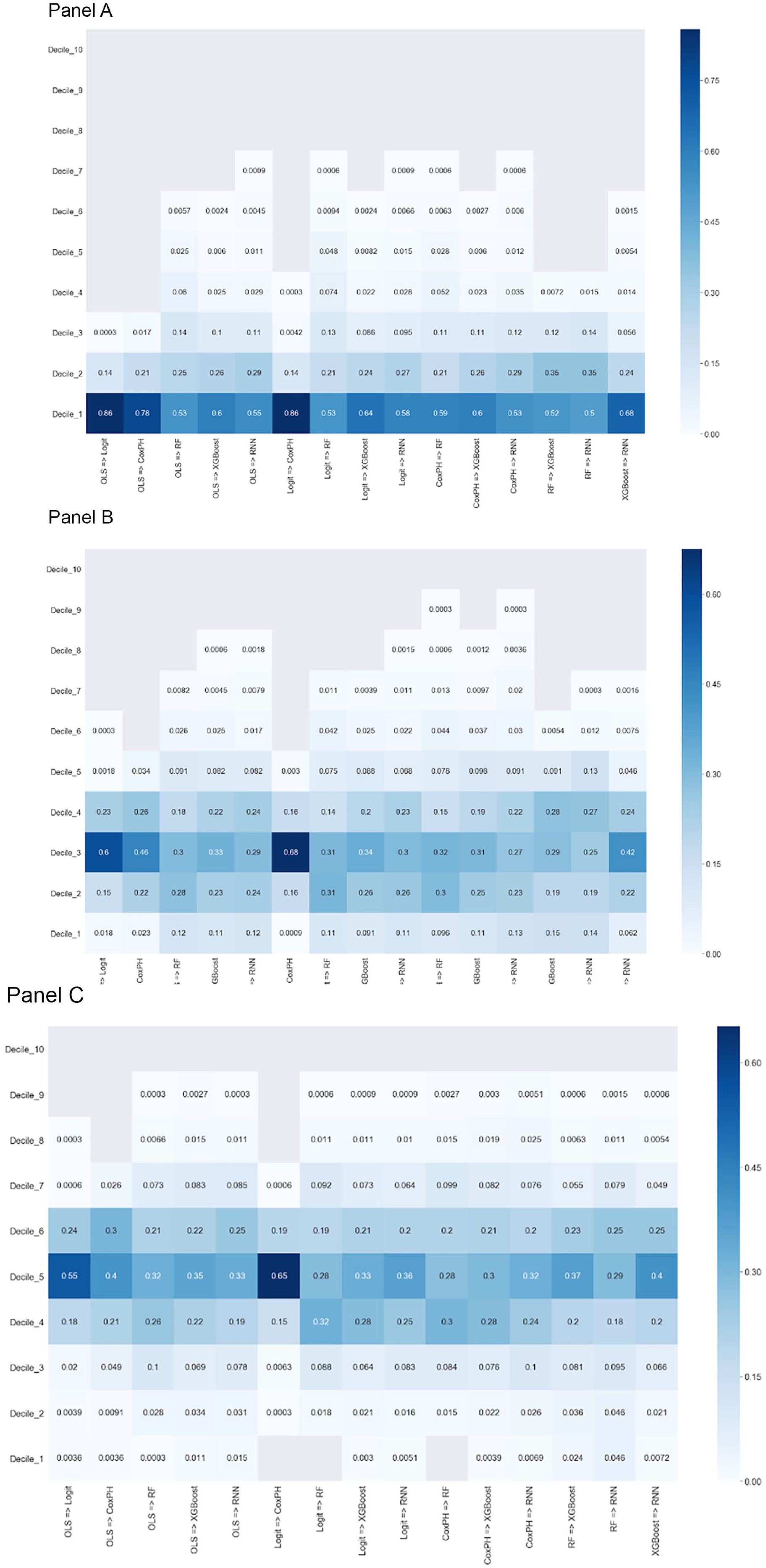
Consistency across models in student assignment to decile of risk rankings. Panel A: first decile of risk rankings; Panel B: third decile of risk rankings; and Panel C: fifth decile of risk rankings.

Despite the instability in relative risk rankings, Figure 7 shows that the share of students assigned to the bottom and third decile who do not graduate is similar across all six base models. This indicates that the models perform similarly well at sorting nongraduates into the bottom and third decile of the risk ranking distribution, but which students are assigned to those deciles differ. This arises because all the models perform similarly at predicting risk in the bottom third of the risk distribution; as a result, we are not able to make value judgments about the differences in model-derived risk rankings, despite the nontrivial instability in risk rank ordering across models. By comparison, Figure 7 shows that the share of students who did not graduate assigned to the fifth decile varies more across the six base models, ranging from 82.9% for the logit model to 86.6% for the XGBoost model. The differences in model-derived risk rankings between the regression models and the more sophisticated prediction methods are partly explained by the increased prediction accuracy of the more sophisticated methods for students on the margin of not graduating.

Figure 7.

Percent of nongraduates within the first, third, and fifth deciles of risk rankings.

Part of the movement across risk deciles is also likely attributable to the fact that, while the models exhibit similar levels of accuracy, they assign different levels of importance to the predictors to generate predictions. Figure 8 shows the degree of overlap of the top 20% of predictors based on their feature importance across model pairs.¹⁵ While the level of overlap is relatively high between the regression-based (62%) and tree-based models (77%), the cross-family pairs share fewer than 35% of the most important predictors in common. In sum, our analysis shows that students’ predicted risk of not graduating can vary meaningfully across modeling strategies. For researchers and administrators, this instability means that modeling selection can significantly affect which students receive outreach and support if resource constraints prohibit colleges from intervening with all students predicted not to graduate. We discuss the practical implications of these results in the “Results” section.

Figure 8.

Commonality of top 20% of important features across base models.

Models With a Reduced Set of Predictors or a Reduced Sample Size

As we describe in the “Empirical Strategy” section above, we incorporate 331 predictors into the base models. Furthermore, after exploring the complexity of variable construction in section “Outcome Variable Definition,” we concluded that the performance of models is largely unaffected by the exclusion of complexly specified term-specific predictors from the base models. In the section “Outcome Variable Definition,” we also showed that models experience more significant reductions in performance when simple term-specific predictors and complexly specified non-term-specific predictors are excluded. In the online Supplemental Appendix 5 we further investigate changes to model performance when restricting the set of predictors by examining the stability of risk rankings across the base models and models that include fewer predictors. The results of that analysis reveal that excluding predictors that have negligible impact on model performance (e.g., the complexly specified term-specific predictors) only leads to a modest change in the risk rank ordering of students, with the OLS and logistic regression models exhibiting greater stability in risk rankings than other models. We also find that excluding all term-specific predictors leads to more significant changes in the rank ordering of students, with the tree-based methods exhibiting greater stability in risk rankings than the regression methods. The tree-based methods generate more stable risk rankings in this context because they exhibit better prediction accuracy than regression methods when term-level predictors are excluded from the prediction models.

We also tested how the base models perform in much smaller settings, limiting the data to one medium-sized VCCS college and separately to a 10% random sample of the data. We find that, despite the significant reductions in sample size, models applied to smaller samples perform similarly well compared with the base models in larger samples.¹⁶ However, once again we find that the risk rank ordering of students changes substantially in smaller versus larger samples. This is especially true for the tree-based methods. We discuss these results in more detail in the online Supplemental Appendix 6.

Preliminary Investigation of Bias in Predictive Models

While a full investigation of potential bias within predictive models—and potential strategies to mitigate that bias—is beyond the scope of this article, we do provide a preliminary exploration of potential bias given the common concern that predictive modeling in education may be biased against subgroups with historically lower levels of academic achievement or attainment (see, e.g., Ekowo & Palmer, 2016). To illustrate this issue, Figure 9 shows the actual graduation rates of students in our validation sample, by gender, race/ethnicity, Pell status, age, and first-generation status. We see that many historically disadvantaged groups—including Black and Hispanic students, Pell recipients, first-generation college goers, and older students—have significantly lower graduation rates compared with their more privileged counterparts. Including these types of demographic characteristics in predictive models can result in historically disadvantaged subgroups being assigned a lower predicted probability of graduation, even when members of those groups are academically and otherwise identical to students from more privileged backgrounds.¹⁷ Removing demographic predictors is an intuitive approach to addressing concern of bias in predictive models; researchers and administrators might reason that, without demographic predictors in the model, students with the same academic performance backgrounds would be assigned the same predicted score, regardless of race, age, gender, or income. Furthermore, some state higher education systems and individual institutions face legal obstacles or political opposition to including certain demographic characteristics in predictive models (Baker, 2019; Blume & Long, 2014). We therefore examine how excluding demographic predictors affects the performance and student-specific risk rankings of the base models.

Figure 9.

Graduation rates by subgroup.

Figure 10 compares the c-statistic and nongraduation F1-score values of the base models with models that exclude the following demographic characteristics: race/ethnicity, gender, Pell eligibility, age, and first-generation status. Despite the strong relationship between these demographic characteristics and graduation shown in Figure 9, the accuracy of all the models is virtually unchanged (the performance metrics all change by less than 1%) when demographic characteristics are excluded. This occurs because many of the nondemographic predictors that remain in the model are highly correlated with both student demographic characteristics and the probability of graduation. We show this explicitly by identifying the top 20 predictors in terms of feature importance from the XGBoost model that excludes demographic characteristics.¹⁸ We then compare the mean values of those predictors for Black versus non-Black students, and for older (age 25 years and up) versus younger students. Table 2 shows that there are large and statistically significant differences between Black and non-Black students and between older and younger students across nearly all 20 predictors. For example, in row 2 of Table 2, Black students have a cumulative GPA of 2.13 on average compared with 2.63 among non-Black students; the difference of 0.51 grade points is significant at the 1% level.¹⁹ In other words, even when race is not incorporated into prediction models explicitly, the results still reflect the factors that drive race-based differences in educational attainment seen in Figure 9. While full exploration of potential bias in predictive modeling is beyond the scope of this article, we view this as an important area for further study. We also provide a detailed discussion of the effect of removing demographic predictors from base models on the movement of students across the distribution of risk rankings in the online Supplemental Appendix 5.

Figure 10.

Evaluation statistics, base models versus models excluding demographic predictors.

Table 2

Racial and Age Differences in the 20 Most Important Features

Predictor	Black	Non-Black	Difference	Age 25+ years	Age <25 years	Difference
Slope of term GPA	−0.169	−0.136	−0.033***	−0.149	−0.143	−0.007
Cumulative GPA	2.126	2.631	−0.505***	2.801	2.364	0.438***
Slope of term-level number of credits attempted	−0.521	−0.504	−0.017	−0.352	−0.581	0.23***
Percentage of attempted credits that were withdrawn	0.118	0.086	0.032***	0.082	0.1	−0.019***
Percentage of attempted credits that were 200-level courses	0.197	0.223	−0.026***	0.233	0.209	0.025***
Percentage of attempted credits that were developmental courses	0.226	0.135	0.091***	0.151	0.162	−0.011***
Percentage of attempted credits that were completed	0.694	0.81	−0.116***	0.843	0.752	0.091***
Total grant dollars received in first year	2001	1219	781.3***	1432	1414	18.31
Standard deviation of term-level share of attempted credits that were withdrawn	0.161	0.127	0.034***	0.121	0.141	−0.021***
Credits attempted in first Fall term	9.058	10.064	−1.006***	7.979	10.592	−2.613***
Standard deviation of term-level share of attempted credits that were completed	0.225	0.164	0.061***	0.13	0.2	−0.07***
Term-level GPA in first Fall term	2.408	2.759	−0.351***	3.142	2.494	0.648***
Credits attempted in first Spring term	9.472	10.154	−0.683***	8.406	10.631	−2.225***
Term-level GPA in first Spring term	2.365	2.724	−0.359***	3.166	2.436	0.73***
Credits attempted in second Fall term	6.24	7.272	−1.032***	5.318	7.73	−2.412***
Term-level GPA in second Fall term	2.344	2.654	−0.31***	3.012	2.447	0.565***
Credits attempted in first Spring term	6.961	6.658	0.304**	6.333	6.852	−0.519***
Credits attempted in first Summer term	3.287	2.864	0.423***	4.168	2.535	1.633***
Total grant dollars received in second year	2603	1394	1210***	2213	1445	767.8***
Term-level GPA in second Spring term	2.473	2.724	−0.252***	3.111	2.501	0.609***

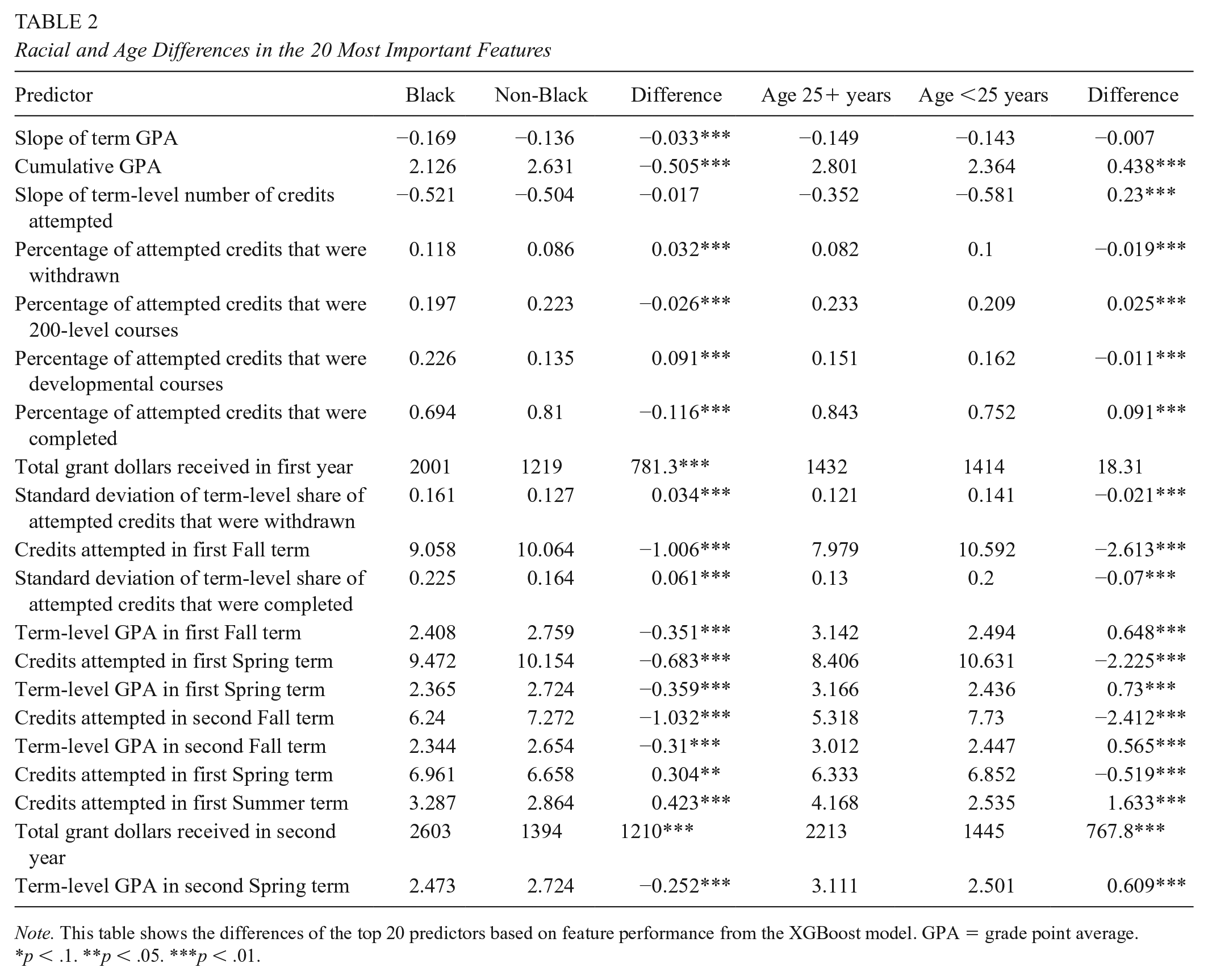
Note. This table shows the differences of the top 20 predictors based on feature performance from the XGBoost model. GPA = grade point average.

p < .1. **p < .05. ***p < .01.

Discussion

In an era when colleges and universities are facing mounting pressure to increase completion rates, yet public funding for higher education is being cut, institutions have embraced predictive analytics to identify which students to target for additional support. We evaluated the performance of different approaches to sample and variable construction and to different modeling approaches to better understand the trade-offs to modeling choices. Perhaps the most salient finding from our analysis is that, for a given student, the notion of “risk” is not stable and can vary meaningfully across the modeling strategy used. This instability is most pronounced when compared with tree-based and neural network modeling approaches, and among students with more moderate risk of withdrawal prior to completion. For instance, across model pairs, fewer than 70% of students assigned a risk rating in decile 3 by one model were also assigned to decile 3 by the other model.

The evidence in this study does suggest that institutions would realize important gains in model accuracy through thoughtful sample and predictor construction. In general, more sophisticated tree-based models differentiate between graduates and nongraduates more accurately than simpler regression-based models, although the gains in accuracy are small. More complex models also generate student risk rankings whose ordering is more sensitive to modeling choices, such as which predictors are included in the models or which institutions or students are included in the sample.

Given these findings, a natural question is under what conditions should colleges consider using tree-based versus regression-based models for targeting purposes. In technical terms, our results suggest that sophisticated machine learning approaches offer a slight advantage when colleges use predictions to target students broadly. The subset of students flagged for intervention is not likely to change considerably in those circumstances, even when different modeling choices produce moderate changes to student risk rankings. Our results also suggest that the value of using tree-based prediction models increases when institutions have limited choice over modeling decisions (e.g., due to legal restrictions over the inclusion of student attributes or because of data limitations). Alternatively, rank order stability becomes more consequential when colleges can only target a small subset of students for additional support; in such cases, we find that OLS and logistic regression models have a comparative advantage.

There are a broader set of questions that are important for institutions to consider when making decisions about using predictive analytics in higher education. Regardless of modeling approach, there are numerous important ethical considerations. One relates to the bias issue; as we show above, students from underrepresented groups are likely to be ranked as less likely to graduate regardless of whether demographic measures are included in the models. On the positive side, this could lead to institutions investing greater resources to improve outcomes for traditionally disadvantaged populations. But there is also the potential that outreach to underrepresented students could have unintended consequences, such as reinforcing anxieties students have about whether they belong to the institution. This could exacerbate existing equity gaps within institutions (Barshay & Aslanian, 2019; Walton & Cohen, 2011). There are also important ethical questions around the data elements that institutions incorporate into their predictive models, and whether students are aware of and would consent to these uses of data (Brown & Klein, 2020). For instance, researchers at the University of Arizona use ID swipes to monitor student movement around campus, including when students depart from and return to their dorms (Barshay & Aslanian, 2019). While these measures have the potential to contribute meaningfully to model accuracy, they raise important issues around student privacy that higher education administrators should actively consider.

A second question is whether the benefits of predictive modeling outweigh the costs. To inform this question, we conduct a back-of-the-envelope benefit–cost calculation, which we describe in more detail in the online Supplemental Appendix 8. In the context of a community college with 5,000 students, our estimates of model accuracy imply that using a more advanced prediction method like XGBoost would translate into the institution correctly identifying an additional 64 at-risk (i.e., nongraduating) students compared with OLS. If realizing this improvement requires the purchase of proprietary predictive modeling services, the average cost to colleges is estimated to be $300,000.²⁰ This implies an average cost per additional correctly identified at-risk student of $4,688. While this is solely a back-of-the-envelope calculation, we believe it nonetheless illustrates the importance of higher education leaders critically evaluating whether the gains from more sophisticated approaches to predictive analytics are likely to be greater than what could be realized from alternative investments of those resources.

A final question is whether predictive analytics are actually resulting in more effective targeting of and support for at-risk students in higher education. While few studies to date have examined the effects of predictive analytics on college academic performance, persistence, and degree attainment, the three experimental studies of which we are aware find limited evidence of positive effects for at-risk students (Alamuddin et al., 2019; Milliron et al., 2014; Plak et al., 2019). More research is needed to understand the role of predictive analytics in improving institutional performance. One challenge to identifying the impacts of predictive analytics on student outcomes is that it is easy to conflate the targeting value of predictive modeling with the efficacy of interventions built around its use. The slightly positive or null effects found in previous studies may reflect that predictive models convey limited information about students on which institutions can act. Alternatively, even if predictive models contain actionable information, coupling data analytics with ineffective interventions could conceal the targeting value of predictive analytics. One approach to isolating the targeting value of predictive modeling is to examine whether intervention effects vary by model-generated predictions. To our knowledge, prior research has not examined this question and it merits attention in future work. More work is also needed to understand the extent to which predictive modeling in higher education suffers from algorithmic bias and whether that diminishes the efficacy of predictive modeling for historically underserved groups.

In conclusion, the findings in this article reveal that institutional leaders should carefully consider the intended uses for predictive modeling in their local context before choosing to invest in expensive predictive modeling services.

Supplemental Material

sj-docx-1-ero-10.1177_23328584211037630 – Supplemental material for Bringing Transparency to Predictive Analytics: A Systematic Comparison of Predictive Modeling Methods in Higher Education

Supplemental material, sj-docx-1-ero-10.1177_23328584211037630 for Bringing Transparency to Predictive Analytics: A Systematic Comparison of Predictive Modeling Methods in Higher Education by Kelli A. Bird, Benjamin L. Castleman, Zachary Mabel and Yifeng Song in AERA Open

Footnotes

Acknowledgements

We are grateful for our partnership with the Virginia Community College System and in particular Dr. Catherine Finnegan. We are grateful to the Lumina, Overdeck, and Heckscher Family Foundations for the financial support. Any errors are our own.

1.

Among students who earn a credential within 6 years in our sample, 31% earn their credential from a non-VCCS institution. An additional 18% of graduates earn a credential from both a VCCS and a non-VCCS institution within 6 years. For our earliest cohort of students (those initially enrolled during the 2007–2008 academic year), we observe 78.4% of all eventual degree completions through the last term of data available (spring 2018) within 6 years of initial enrollment. And while a sizable share of VCCS students intend to transfer to a 4-year institution before earning their VCCS credential and bachelor’s degrees are typically designed to be completed within 4 years, more than half of bachelor’s degree–seeking students take more than 4 years to graduate (Shapiro et al., 2016); time to bachelor’s degree is longer for community college transfer students (Lichtenberger and Dietrich, 2017).

2.

90/10, 80/20, 70/30 are all typical ratios used to split samples into training/validation sets. The smaller the validation set, the more likely measurement error will degrade the evaluation of model performance. At the same time, a smaller validation set increases the size of the training set, which enables development of more informative prediction models. In the context of this study, because more than 30,000 students are included in the validation sample based on the 90/10 ratio, the validation sample is sufficiently large for evaluating model performance reliably and allows us to include more observations in the training sample to maximize prediction precision.

3.

In other words, all predictive models have the possibility of fitting the training set well but not performing equally well on the unseen data, which is caused by the model tendency to pick up the idiosyncrasies/noises from the finite training set during the model fitting procedure. So it is necessary to withhold part of the full data as the validation set to avoid overestimating model performance.

4.

OLS, also known as a linear probability model in the context of a binary outcome variable, may not conform with all theoretical assumptions of a classification model (e.g., the predicted scores are not bound to fall between 0 and 1). Still, it is the predictive model that typically requires the least computing power and offers the highest degree of interpretability.

5.

Discrete time survival analysis methods would also be appropriate since we observe data in term intervals. However, we employ CPH to model graduation as a function of continuous time because it is easy to implement, widely used in the field, and from a practical perspective, the predictions generated from discrete-time and continuous-time methods are virtually identical in most applications (Mills, 2011; Singer & Willett, 2003).

6.

For example, implementation of these methods requires execution of model tuning and cross-validation procedures. We follow conventional standards of practice in machine learning for tuning and cross-validation and discuss those procedures in detail in the .

7.

Following convention, we explored feature selection for the regression and tree-based models as a preprocessing step with the goal of removing potentially irrelevant predictors that could diminish model performance. However, model performance did not improve as the number of predictors decreased in the feature selection routine, which suggests there are essentially no noisy predictors present in the full-predictor model.

8.

We provide a more detailed description of each evaluation statistic in the .

9.

RNN models are not applicable for this analysis because time-dependent predictors are excluded from the models used for testing full versus truncated samples. Furthermore, we do not estimate CPH models using the nontruncated sample due to the particular sample construction procedures we employed for survival analysis modeling. We refer the reader to the section on CPH modeling in the for further details.

10.

We do not test the comparison of full versus truncated sample construction for models that include term-specific predictors, because when using the nontruncated training sample, there is no reliable and robust way of imputing term-specific predictor values in unobserved terms for observations in the validation sample. Furthermore, even though we could apply missing value imputation methods to the validation sample, this would not resolve the fact that the distribution of enrollment durations for students in nontruncated samples do not resemble those of currently enrolled students. As a result, we expect that nontruncated samples with imputed term-level predictors would perform worse than truncated samples, as is observed in the case of models that only use non-term-specific predictors.

11.

Our hypothesis as to why RNN does not significantly outperform the simpler models in this application, while in other applications it often does, is that the average sequence length per student (i.e., the number of actively enrolled terms) is too low to benefit from the sequential structure of the RNN model. One third of students in the training sample have only one time step, 60% have fewer than three time steps, and 79% have fewer than five time steps. Prior research has found that increased sequence length in the training sample leads to improved prediction accuracy of RNN models (Jafariakinabad et al., 2019; Suzgun et al., 2019).

12.

Given the relatively skewed distribution of the graduation outcome, we tested whether upweighting the observations of actual graduates improved model performance. It did not.

13.

For the same model, precision and recall move in opposite directions as the threshold of predicted scores used to categorize students as either at-risk or not at-risk changes. For instance, the nongraduation value increases as the threshold increases, because more actual nongraduates will be correctly identified. At the same time, nongraduation precision will decrease because the higher threshold will predict that more actual graduates will not graduate. For example, the random forest model has the lowest value of graduation precision and the middle values of graduation recall and graduation F1-score.

14.

In online Supplemental Appendix Table A2, we report Person’s and Spearman’s rank correlation coefficients across the models. The correlations range from 0.92 to 0.99, indicating a relatively high level of consistency in rank orderings across the models and the full distribution of risk rankings. However, as shown in , the correlations mask nontrivial differences in percentile rankings between model pairs for some students.

15.

Feature importance measures the contribution of each predictor to the construction of predicted probabilities. The CPH and RNN models are excluded from the results in because those prediction methods do not generate feature importance measures.

16.

Due to the pattern of results we observe across the regression and tree-based models, and given the substantial time required to fit and fine-tune the RNN models, we did not perform this additional analysis for the RNN model.

17.

This source of bias would likely result in students from historically disadvantaged groups being more likely to be identified as at-risk of not graduating and targeted for additional resources. While that might appear to benefit students from historically disadvantaged groups, increased intervention could be detrimental if, for example, outreach from college administrators reinforces students’ anxieties about their potential for college success and thus increases their probability of dropout (Steele & Aronson, 1995; Walton and Cohen, 2011). More broadly, this type of bias would also result in a less efficient distribution of scarce institutional resources to support students.

18.

We focus on the top 20 predictors in terms of feature performance from the XGBoost model because that model demonstrates the highest overall level of accuracy.

19.

In , we further show that there is almost complete overlap (92%–94%) in terms of the predictors with highest feature performance between the base models and models that exclude demographic characteristics. This reinforces that excluding demographic characteristics makes very little change to the risk levels assigned to different groups of students.

20.

This cost is reported by James Wiley, a technology analyst with Eduventures, in .

Authors

KELLI A. BIRD is a research faculty member at the University of Virginia. Her research focuses on policies and strategies to increase postsecondary educational attainment.

BENJAMIN L. CASTLEMAN is the Newton and Rita Meyers Associate Professor in the Economics of Education at the University of Virginia. His research focuses on data and behavioral science strategies to improve educational and workforce success.

ZACHARY MABEL was an associate policy research scientist at the College Board. He is a research professor of education and economics at Georgetown University. His research focuses on policies and strategies to increase postsecondary educational attainment.

YIFENG SONG is a data scientist at the University of Virginia. His research focuses on applying data science methods to education and public policy topics.

References

Abu-Mostafa

Y. S.

Magdon-Ismail

Lin

H. T.

(2012). Learning from data. http://amlbook.com/

Alamuddin

Rossman

Kurzweil

(2019, June 27). Interim findings report: MAAPS advising experiment. Ithaka S+R. https://sr.ithaka.org/publications/interim-findings-maaps-advising-experiment/

Association of Public & Land-Grant Universities. (2016). Congress should lift the ban on student level data in HEA reauthorization (Policy Brief). https://www.aplu.org/library/congress-should-lift-the-ban-on-student-level-data-in-hea-reauthorization/File

Attewell

Monaghan

D. B.

(2015). Data mining for the social sciences. University of California Press.

Bailey

M. J.

Dynarski

S. M.

(2011). Inequality in postsecondary education. In Duncan

G. J.

Murnane

R. J.

(Eds.), Whither opportunity (pp. 117–132). Russell Sage Foundation.

Baker

D. J.

(2019). Pathways to racial equity in higher education: Modeling the antecedents of state affirmative action bans. American Educational Research Journal, 56(5), 1861–1895. https://doi.org/10.3102/0002831219833918

Barshay

Aslanian

(2019). Under a watchful eye: Colleges are using big data to track students in an effort to boost graduation rates, but it comes at a cost (APM Reports). https://www.apmreports.org/story/2019/08/06/college-data-tracking-students-graduation

Bastrikin

(2020). Student loan debt statistics. https://educationdata.org/student-loan-debt-statistics/#

Blume

G. H.

Long

M. C.

(2014). Changes in levels of affirmative action in college admissions in response to statewide bans and judicial rulings. Educational Evaluation and Policy Analysis, 36, 228–252. https://doi.org/10.3102/0162373713508810

10.

Breiman

Friedman

J.H.

Olshen

Stone

(1984). Classification and regression trees. Wadsworth & Brooks, Pacific Grove. https://www.taylorfrancis.com/books/9781315139470

11.

Brown

Klein

(2020). Whose data? Which rights? Whose power? A policy discourse analysis of student privacy policy documents. Journal of Higher Education, 91(7), 1149–1178. https://doi.org/10.1080/00221546.2020.1770045

12.

Burke

Parnell

Wesaw

Kruger

(2017). Predictive analysis of student data: A focus on engagement and behavior. The National Association of Student Personnel Administrators. https://www.naspa.org/images/uploads/main/PREDICTIVE_FULL_4-7-17_DOWNLOAD.pdf

13.

Che

Purushotham

Cho

Sontag

Liu

(2018). Recurrent neural networks for multivariate time series with missing values. Scientific Reports, 8, Article 6085, https://doi.org/10.1038/s41598-018-24271-9

14.

Chetty

Friedman

J. N.

Saez

Turner

Yagan

(2020). Income segregation and intergenerational mobility across colleges in the United States. Quarterly Journal of Economics, 135(3), 1567–1633. https://doi.org/10.1093/qje/qjaa005

15.

Complete College America. (2014). Four-year myth: Make college more affordable. Restore the promise of graduating on time. https://eric.ed.gov/?id=ED558792

16.

Deming

D. J.

Walters

C. R.

(2017). The impact of price caps and spending cuts on U.S. postsecondary attainment (NBER Working Paper No. 23736). National Bureau of Economic Research.

17.

Ekowo

Palmer

(2016, October). The promise and peril of predictive analytics in higher education: A landscape analysis (New America Policy Paper). https://www.newamerica.org/education-policy/policy-papers/promise-and-peril-predictive-analytics-higher-education/

18.

Hand

Mannila

Smyth

(2001). Principles of data mining. MIT Press.

19.

Herzog

(2006). Estimating student retention and degree completion time: Decision trees and neural networks vis-a-vis regression. New Directions for Institutional Research, 131(Fall), 17–33. https://doi.org/10.1002/ir.185

20.

Jafariakinabad

Tarnpradab

Hua

K. A.

(2019). Syntactic recurrent neural network for authorship attribution. arXiv:1902.09723. https://arxiv.org/abs/1902.09723

21.

James

Witten

Hastie

Tibshirani

(2013). An introduction to statistical learning: With applications in R. Springer.

22.

Karpathy

(2015, May 21). The unreasonable effectiveness of recurrent neural networks [Blog post]. http://karpathy.github.io/2015/05/21/rnn-effectiveness/

23.

Klempin

S. C.

Grant

Ramos

(2018). Practitioner perspectives on the use of predictive analytics in targeted advising for college students (CCRC Working Paper No. 103). https://ccrc.tc.columbia.edu/publications/practitioner-perspectives-predictive-analytics-targeted-advising.html

24.

Lichtenberger

E. l.

Dietrich

(2017). The community college penalty? Examining the bachelor’s completion rates of community college transfer students as a function of time. Community College Review, 45(1), 3–32. https://doi.org/10.1177/0091552116674550

25.

Looney

Yannelis

(2015). A crisis in student loans? How changes in the characteristics of borrowers and in the institutions they attended contributed to rising loan defaults (Brookings Papers on Economic Activity). Brookings Institution Press.

26.

Baum

Pender

Welch

(2017). Trends in college pricing. College Board.

27.

Milliron

M. D.

Malcolm

Kil

(2014). Insight and action analytics: Three case studies to consider. Research & Practice in Assessment, Winter, 70–89.

28.

Mills

(2011). Introducing survival and event history analysis. Sage. https://dx.doi.org/10.4135/9781446268360

29.

Paterson

(2019, April 18). What a predictive analytics experiment taught 11 colleges about sharing data. Higher Ed Dive. https://www.highereddive.com/news/what-a-predictive-analytics-experiment-taught-11-colleges-about-sharing-dat/552986/

30.

Plak

Cornelisz

Meeter

van Klaveren

(2019). Early warning systems for more effective student counseling in higher education: Evidence from a Dutch field experiment. Amsterdam Center for Learning Analytics and Vrije Universiteit Amsterdam.

31.

Shapiro

Dundar

Wakhungu

P. K.

Yuan

Nathan

Hwang

(2016, September). Time to degree: A national view of the time enrolled and elapsed for associate and bachelor’s degree earners (Signature Report No. 11). National Student Clearinghouse Research Center.

32.

Singer

J. D.

Willett

J. B.

(2003). Applied longitudinal data analysis: Modeling change and event occurrence. Oxford University Press. https://doi.org/10.1093/acprof:oso/9780195152968.001.0001

33.

Stark

(2015, September 14). Leveraging analytics in community colleges. EDUCAUSE Review. https://er.educause.edu/articles/2015/9/leveraging-analytics-in-community-colleges

34.

Steele

C. M.

Aronson

(1995). Stereotype threat and the intellectual test performance of African Americans. Journal of Personality and Social Psychology, 69(5), 797–811. https://doi.org/10.1037/0022-3514.69.5.797

35.

Suzgun

Belinkov

Sieber

S. M.

(2019). On evaluating the generalization of LSTM models in formal languages. Proceedings of the Society for Computation in Liguistics (SCiL), pp. 277–286. https://doi.org/10.7275/s02b-4d91

36.

Treaster

J. B.

(2017, February 2). Will you graduate? Ask big data. The New York Times. https://www.nytimes.com/2017/02/02/education/edlife/will-you-graduate-ask-big-data.html?_r=1

37.

U.S. Department of Education. (2019). The condition of education: College enrollment rates. https://nces.ed.gov/programs/coe/indicator_cpb.asp

38.

Walton

G. M.

Cohen

G. L.

(2011). A brief social-belonging intervention improves academic and health outcomes of minority students. Science, 331(6023), 1447–1451.

Supplementary Material

Please find the following supplemental material available below.

For Open Access articles published under a Creative Commons License, all supplemental material carries the same license as the article it is associated with.

For non-Open Access articles published, all supplemental material carries a non-exclusive license, and permission requests for re-use of supplemental material or any part of supplemental material shall be sent directly to the copyright owner as specified in the copyright notice associated with the article.

0.00 MB

3.17 MB