Sage Journals: Discover world-class research

Abstract

State policymakers wrestle with long-standing questions and concerns about how to best provide additional fiscal support to rural school districts to ensure their students have access to adequate educational opportunities. In this study, we describe how one state developed empirically based estimates for the additional cost of operating rural schools, typified by small enrollment and location in sparsely populated areas. The study’s findings clarify that school size and location are relevant, but distinct, cost factors that should be accounted for state school finance policies. Additionally, the study provides a model for how other states might leverage administrative data and apply education cost modeling to estimate cost differences for rural schools that can be used to inform state school finance policy.

Keywords

education cost modeling rural schools K–12 school finance state policy

Most states provide some form of supplemental funding to small, rural, or geographically isolated school districts to offset the higher costs of operating schools in these contexts. Cost differences stem from the availability and price of key educational resources, the cost of operating comparatively smaller schools, and student transportation (Sipple & Brent, 2015). Yet state policies that provide supplemental and categorical aid to rural schools have been criticized for not reflecting the actual level of need or cost of educating students in rural schools, and as a result, falling short of ensuring that students who attend schools in rural communities have access to educational opportunities on par with those of their peers who attend nonrural schools (Baker & Duncombe, 2004; Malhoit, 2005; Strange, 2011).

In a perfect world, state funding policies would ensure that all schools, including those in rural areas, have the resources necessary for all students to achieve common outcome standards set by the state. Failing to do so runs the risk of undermining a state’s responsibility to provide an adequate education for all students (Duncombe et al., 2015). To make policy, however, states need to know how much money each school needs to meet these goals. Establishing the cost of an adequate education has been the focus of K–12 education policy research for several decades, and policy advisement studies have been conducted in most states nationwide. Yet the focus of this work has largely been on estimating the base, or average, cost of education for the typical student or school districts and differences from this base attributable to dissimilarities in student need and input prices (e.g., teacher salaries; Aportela et al., 2014). When considered, economies of scale and district or school location were most frequently included as mediating factors, not as explicit sources of variation in cost across districts or schools.

In this article, we describe the approach used to estimate cost differentials for small, rural schools in Vermont. More than half of Vermont’s students attend school in an area where small, geographically isolated schools are the norm (Showalter et al., 2019). This study responds to Vermont policymakers’ interest in considering whether weights should be added to the state’s school funding formula for school size and location, after controlling for other cost factors. Specifically, we leverage data from state and national databases and use cost function analysis—specifically education cost modeling (ECM)—to identify specific factors associated with differences in the cost of achieving common outcome goals across Vermont schools and estimate each factor’s cost differential. Additionally, we demonstrate how the policy application of ECM extends beyond identifying specific cost adjustments to specifying understandable and usable weights that can be incorporated in state school funding formulae.

Conceptual and Empirical Background

Scale and Geographic Location as Cost Factors

States are responsible for providing an adequate education for all students. However, not all students have the same learning needs or backgrounds and require different types and levels of educational supports to achieve standards or outcomes deemed adequate. Similarly, districts and schools that operate in different contexts may also require varying levels of resources because of scale of operations or the price they must pay for key resources. As a result, providing an adequate education to all students necessarily means that resources should differ across school districts according to differences in educational costs.

Differences in educational costs across school districts can be conceptualized as a set of cost factors that affect the level of spending required for all students to achieve specified outcomes and that are outside the control of local district and school administrators (Baker, 2018; Duncombe et al., 2015; Table 1). Among cost factors, school district size and location are recognized as an independent source of variation in cost. Districts or schools with limited enrollment may be unable to achieve economies of scale (Andrews et al., 2002). For example, school districts with fewer than 100 students may be as much as two times more expensive to operate than districts with more than 2,000 pupils, and 50% more than districts with 100 to 300 students (Baker & Duncombe, 2004). Doubling enrollment in a 300–pupil district may reduce operating costs per pupil by about 62% and 50% for a 1,500–pupil district (Duncombe & Yinger, 2007). District and school location may also affect educational costs. Schools in sparsely populated areas, or where there are geographic barriers, can pay higher input prices for specific goods or services due to limited supply or the additional cost of transporting resources to the school (Sipple & Brent, 2015).

Table 1

Factors That Account for Differences in Education Costs Across Districts and Schools

Student need	Scale and location	Grade range	Price level of inputs
Individual student characteristics • Economic disadvantage • Disability status • English language learners (ELLs) • Gifted and talented Collective population characteristics • Concentrations of students living in poverty or ELL students	• District or school enrollment • Population sparsity or extent of rurality	• Differences in academic and nonacademic programming for students in different grades	• Geographic differences in resources, including personnel wages and non-personnel resources

Most state school funding programs make one or more adjustments for differences in costs across districts and schools for variation in economies of scale, or geographic location (Table 2). For the 2018 academic year, 13 states included cost adjustments for the geographic location or population density of the community in which a district or school is located. State polices differed in how they measured population density and the threshold used to identify sparsely populated areas. In addition to population density, some state policies also incorporate criteria based on a school district’s physical geography, or the driving distance between districts or schools (e.g., Arkansas, Colorado, Nebraska).

Table 2

Fifty–State Summary of Cost Adjustments for Scale, Sparsity, and Transportation

Cost adjustment	Total number of states applying adjustment	Adjustments to base amount				Discretionary grant program or appropriation
Cost adjustment	Total number of states applying adjustment	Single weight	Multiple weights	Resource-based allocation	Flat grant per pupil	Discretionary grant program or appropriation
Geographic isolation or population density	13	4 (AR, FL, ND, NE)	4 (AK, AZ, NY, SD)	2 (ID, WV)	1 (FL)	2 (MI, TX)
District or school enrollment	26	4 (IA, OK, PA, WV)	8 (AK, AR, AZ, KS, LA, ND, NM, TX)	5 (NC, SD, UT, WA, WY)	4 (MN, MO, OR, WI)	5 (CA, GA, ID, MI, VT)
Adjustment for enrollment is applied only to districts/schools that are also geographically isolated	13	AR, AZ, CA, FL, ME, MI, MN, NC, OR, PA, UT, WI, WV
Operates Transportation Grant/Aid Program	43	AK, AL, AR, AZ, CA, CO, DE, FL, GA, HI, ID, IA, IL, KS, KY, LA, MA, MD, ME, MI, MN, MO, MS, NC, ND, NE, NJ, NM, NV, NY, OH, OK, OR, PA, RI, SC, TN, TX, UT, VT, WA, WI, WY

Note. Sources: The summary of state policies is based on information reported by (a) EdBuild’s FundEd: State policy analysis (http://funded.edbuild.org/state) and (b) A quick glance at school finance: 50–state survey of school finance policies (https://schoolfinancesdav.wordpress.com). In addition, individual states’ statute and other documents were reviewed when further information or clarification was needed.

Twenty-six states recognized that small districts and schools are less able to take advantage of economies of scale in operations. Of states that incorporate an adjustment for district or school size in their funding policies, 13 further conditioned funding on whether the district or school was located in a geographically isolated area. States apply different thresholds to determine at what point a district or school becomes sufficiently small to qualify for additional assistance. Most states use student enrollment as an indicator for size but apply different cut-points for receiving aid, and a small number of states set enrollment thresholds according to the number of students in a grade or average class size in a school.

Forty-three states provided supplemental funding for student transportation. Transportation aid usually operates as a categorical grant program, separate from adjustments for school size or population density included in the state aid calculation. The criteria for receiving aid differs considerably across states. Some states reimburse districts for a share of allowable costs, while others condition funding on miles driven, the average distance between students’ homes and schools, or provide a flat grant amount for each student for which a district provides transportation.

Despite the prevalence of cost adjustments in state education funding formula for differences in educational costs due to scale, sparsity, and transportation, state policy is largely made without information on the actual differences in the cost of educating students who attend small and geographically remote districts and schools (Duncombe et al., 2015; Malhoit, 2005). While there is considerable literature on economies of size among educational organizations (Andrews et al., 2002), this body of work primarily speaks to the question of at what point costs differ by size, rather than estimating actual differences in educational costs across school districts of different sizes and locations. Complicating things further is the fact that educational costs represent the minimum spending required to reach a given level of student performance in a particular state. As a result, estimates for education costs are highly dependent on a state’s selected measures of student performance and state context, making it difficult to generalize cost differentials across states (Duncombe et al., 2015).

Measuring Cost Differentials

Over time, K–12 education finance policy research has grown to include multiple approaches to estimating differences in educational costs across districts and schools. Broadly, these approaches fall into one of two categories:

Input-oriented analyses, which identify the resources necessary to produce desired educational outcomes for identified student populations served in various settings, and then assign a dollar value to these resources to estimate educational costs in a prototypical district or school.

Outcome-oriented analyses, which start with student outcomes generated by the programs and services offered by existing schools and districts, and then estimate the statistical relationship between spending on these programs and services and specific outcomes while taking into account different student populations and the characteristics of the settings in which they are being served (Downes & Stiefel, 2015).

The primary methodological distinction between the two approaches rests with the starting point for analysis—that is, whether the analyst starts by specifying inputs and subsequently costing out the value of those inputs, or by designating specific outcome targets and identifying the additional spending necessary to achieve those targets.

Input-Oriented Analyses

Modern input-oriented analysis is grounded in the resource cost modeling (RCM) approach (Chambers, 1999), and begins with goals—or the outcomes the system is intended to achieve—and then asks consultants or expert panels to identify the inputs needed to achieve these goals. Broadly, two preferred methods have emerged for identifying appropriate combinations of resources that will deliver the outcome goals: (1) Professional Judgment (PJ); and (2) Evidence-based (EB), with the former relying on focus groups to propose the resources needed to achieve specific outcomes at prototypical schools in a state and the latter involving the compilation of published research studies on existing school interventions that have been proven effective at producing specific outcomes and deriving from these studies the resources used by these interventions (Downes & Stiefel, 2015). In both instances, the empirical method is for the analyst to tally identified resources, attach prices, and sum costs.

However, even under the best application, the cost estimates resulting from PJ or EB methods represent experts’ judgments or hypotheses about the resources required to produce desired outcome goals (Baker, 2006). There are no guarantees that the identified programs or associated collections of resources necessary to support them are the most efficient manner in which to produce the desired student outcomes. It is also impractical to construct resource models for prototypical district schools across all contexts in a state. This latter critique has proven particularly relevant for costing out educational outcomes in rural and remote school districts; with few exceptions, most existing input-based costing out studies do not explicitly consider differences in resource requirements for small, rural schools districts or those located in sparsely populated areas (Aportela et al., 2014).

Outcome-Oriented Analyses

The primary tool of outcome-oriented cost analysis is the education cost model (ECM). ECM statistically evaluates the relationships between spending levels, outcomes, student needs, and the conditions under which schools operate (e.g., economies of scale) using administrative data from a large number of districts or schools in a state or region (Duncombe & Yinger, 2011). Specifically, ECM estimates a cost function to evaluate the relationship between spending, student outcomes, and other school characteristics:

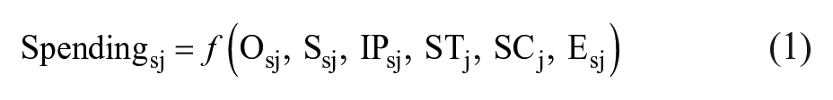
{Spending}_{sj} = f (O_{sj}, S_{sj}, {IP}_{sj}, {ST}_{j}, {SC}_{j}, E_{sj})

(1)

where Spending in school, s, in year, j, is a function of selected student outcomes (O), controlling for a matrix of student need and demographic characteristics (S); Input Prices (IP), measured as geographic variation in the prices of key inputs to schooling such as teacher wages; Structure (ST) is measured as a matrix of district structural characteristics such as grade ranges served in a school; Scale (SC) is a measure of economies of scale usually expressed in terms of student enrollments, and, in some cases, population density; Efficiency (E) is measured as a set of factors that might produce inefficiencies in the spending measure (Duncombe et al., 2015).

This general estimation strategy has been clarified and refined over several decades in its application to estimating cost differentials across districts in multiple states, with the predominant empirical strategy relying on current operating expenditures per pupil as the dependent measure, treating student outcomes as endogenous and incorporating measures of the competitive context as instruments in estimation; and controlling for inefficiencies in the spending measure by including measures of variations in fiscal capacity and public monitoring (e.g., Atchison et al., 2020; Baker, 2011; Chakraborty & Poggio, 2008; Downes & Pogue, 1994; Duncombe & Yinger, 2000, 2005; Gronberg et al., 2011; Imazeki, 2008; Imazeki & Reschovsky, 2003; Kolbe et al., 2019; Zimmer et al., 2009).

The strength of ECM rests with its ability to leverage actual district and school data to model the relationships between educational spending and levels of student outcomes that are informed by state policy (e.g., that equate to students attaining an adequate education), while controlling for identified cost actors (Duncombe & Yinger, 2011). This approach also supports efforts to independently estimate costs for multiple conditions, as well as examine interaction between these factors (Baker, 2018; Downes, 2004). ECM’s ability to isolate cost differentials associated with district or school size or geographic location is particularly relevant for policy advice studies for states, as is its reliance on historical data. Disentangling differences in costs across school districts due to size or location from other cost factors (e.g., student poverty, teacher salaries) is particularly challenging in input-oriented analyses; instead, ECM is able to parse variation in actual district spending attributable to differences in size, structure, and location from other cost factors (e.g., student needs).

That said, there is no single cost model estimation that translates across states or that yields perfect diagnostic features. Instead, ECM estimation is an iterative process that requires balancing technical and statistical concerns with practical application for policymaking. Key challenges include clearly articulating student outcomes or performance objectives and securing data with appropriate district- or school-level measures that are consistent over time (Duncombe & Yinger, 2011). Additionally, not all spending by districts and schools is efficient spending, and instead, in a given district some portion of, but not all, spending contributes directly to measured student outcomes included in the model (Duncombe et al., 2015). However, efficiency cannot be readily observed in the data, and as a result, presents an omitted variable bias problem in cost model estimation—that is, the inability to identify factors that explain differences in spending that are neither associated with legitimate cost differences nor with differences in outcomes such that those factors can be set to a constant level (average) when projecting cost estimates.

The Vermont Policy Context

Vermont’s existing school funding system was put in place as a response to the 1997 Vermont Supreme Court ruling Brigham v. State of Vermont. In this decision, the Court found the existing foundation funding program unconstitutional due to disparities in educational spending between towns with higher and lower property values. The Brigham decision required substantially equal levels of local tax effort for equal levels of school spending and stipulated that the wealth of the state, not local school districts, should pay for local education spending. Vermont’s current school funding system—implemented through Act 60 (1997), Act 68 (2004), and Act 130 (2010)—was designed to simultaneously resolve issues of taxpayer equity and disparities in per pupil spending. Although school budgets are approved by local school district voters, local education spending is funded through a statewide Education Fund, which, among other sources, includes pooled revenues from local education-related property and income taxes.

The State’s existing policy relies on localities to make appropriate adjustments to their annual budget for cost factors (e.g., student risk, social context of schooling, economies of scale), and then adjusts for differences in costs in its funding policy by weighting a district’s average daily membership for cost factors. Districts’ weighted membership is subsequently used to equalize local per pupil spending for the purpose of calculating local tax rates. An equalized pupil can be thought of as an average pupil in terms of educational costs in a school district—that is, an equalized pupil in a school district will have the same cost as any other equalized pupil, even though the actual per pupil cost of individual students varies. In effect, the weighting incorporated in the state’s funding formula implicitly adjusts for spending differences by equalizing per pupil spending across districts according to differences in educational costs. This in turn affects local tax burden to pay for the additional cost of ensuring all students achieve common standards.

Vermont’s existing formula recognizes four categories of students that are presumed to have higher or lower costs (current weighting in parentheses): (1) economically disadvantaged students (1.25), (2) English language learners (1.20), (3) secondary students (1.13), and (4) prekindergarten students (0.46). The weights are used to calculate a district’s long-term weighted PK12 average daily membership (PK12ADM). Since the long-term membership exceeds the number of students in the state, an equalization ratio is calculated, which proportionately deflates the long-term weighted PK12ADM back to the number of students in the state. This deflater is then applied to each school district’s long-term weighted PK12ADM to generate an equalized pupil count for each Vermont school district that is used to calculate an equalized per pupil spending amount which is then used to calculate local education tax rates.

In 2018, Vermont’s Agency of Education (VT AOE) commissioned a study to examine and evaluate the cost factors and weights used in the equalized pupil calculation. Specifically, the study was guided by two questions:

What cost factors should be accounted for in the equalized pupil calculation?

What should the magnitude of the adjustment (or weight) be for each cost factor in the calculation?

In part, the study’s impetus stemmed from concerns about the extent to which the existing funding formula was effective in equalizing educational costs, and by extension, opportunities to learn for students across the state (Kolbe et al., 2019). For the most part, the student need cost factors and weights used in the calculation had not been modified since the funding formula’s inception, despite significant changes in education policy and practice since that time. Additionally, at the time Act 60 was enacted, there was no formal study of the cost factors or differentials across Vermont school districts. Instead, the adopted weights were largely historical artifacts, carried over from the state’s previous foundation formula.

In particular, stakeholders statewide were concerned that the general state aid formula did not explicitly consider cost differentials due to low enrollment and the geographic isolation of rural schools in the state. Vermont is a rural state, with a highly localized education governance system. During FY2018, there were 295 schools in the state, of which all but 19 enrolled less than 1,000 students, and 156 schools enrolled less than 250 students. Since 1998, the state operated a limited categorical grant program that provides additional funding to small, geographically isolated schools (Vermont Agency of Education, n.d.). Identified schools are eligible to receive an additional per pupil grant. Eligibility for the program and the grant award is determined each year based on school enrollment. The state’s Small Schools grant program has been subject to conjecture and criticism for providing insufficient funding to offset the additional cost of operating small, rural schools and for lack of predictability and transparency in both how the state appropriation is determined and funds are ultimately allocated to schools (Kirkaldy, 2015; Kolbe et al., 2019; Picus et al., 2012).

A key consideration for the AOE study of pupil weights was whether the equalized pupil calculation should be revised to incorporate weights for differences in school size and location in lieu of maintaining the state’s existing Small Schools grant program.

Study Design

ECM was used to estimate cost differentials across Vermont schools, including the additional cost of operating small schools and schools in districts located in areas with low population density. Using schools as the unit of analysis provides several advantages in Vermont. First, we were able to more accurately connect resource inputs, student characteristics, and outcome measures, which become complicated with the complex overlay of school districts in Vermont. Estimates at the school level also supported policy recommendations in a state where district governance is shifting—that is, allowing us to combine schools into merged districts where consolidations have occurred. In the sections that follow, we describe the data and methods used in the Vermont school-level model estimation.

Data

The data used in our analyses were derived from the VT AOE’s administrative databases that were merged with extant data from the U.S. Department of Education’s Common Core of Data (CCD), the U.S. Census Bureau’s American Community Survey (ACS), and the Stanford Education Data Archive (SEDA). Given the small number of schools in Vermont, we pooled observations for an 11-year time period (FY 2009–2018). Our models included merged data for 295 Vermont schools that were in operation in 2018. Table 3 lists the measures used in estimating our models.

Table 3

Summary of Measures Used in Analysis

Measures	Description	Source
Total spending per pupil	Total current per pupil operating expenses, divided by the number of students enrolled in a school during the same year.	VT AOE
Student outcomes
Student need
Economic disadvantage	% of students eligible for free-or-reduced price lunch	CCD
English language learners	% of students identified as English language learners	VT AOE
Students with mild disabilities	% of students with specific learning disabilities, speech and language impairments, emotional disturbance, and other health impairments	VT AOE
All other students with disabilities	% of students with all nonmild forms of disabilities	VT AOE
School/district structure
Grade ranges served	Enrollment by grade range (elementary, K–5; middle, 6–8; and secondary grades, 9–12), divided by average daily membership	VT AOE
Scale and sparsity
School size	Indicator for whether a school’s enrollment fell into one of the following categories: <100 students; 101–250 students; >250 students	VT AOE
Geographic isolation	The total population for the geographic area covered by a district divided by the total square miles covered by the district.	VT AOE¹
Input prices
Labor market indicators	In the Vermont school models, four regional indicators were used as controls for differences in local labor markets.	CWI
Labor market indicators	The regional classification was derived from the Education Comparable Wage Index (Taylor & Fowler, 2006), which uses a combination of Core Based Statistical Areas and aggregations of counties based on public use micro data areas in the U.S. Census Bureau’s American Communities Survey.	CWI
Inefficiency measures
Herfindahl Index	Sum of the square enrollment shares across all schools in a district based on average daily membership	VT AOE
County household income	The median income of the households in the county	ACS
Instruments for achievement (used in first-stage equation)
Household income in neighboring districts	The median income of households in the counties of neighboring districts	ACS
Home values in neighboring districts	The median housing value in the counties of neighboring districts	ACS
Average test scores in neighboring districts	Average NAEP-equated test scores from neighboring districts	SEDA

Note. Sources: Vermont Agency of Education (VT AOE) administrative data systems; Comparable Wage Index (CWI; Taylor & Fowler, 2006; Taylor, n.d.); U.S. Census Bureau’s American Communities Survey (ACS); and Stanford Education Data Archives (SEDA). NAEP = National Assessment of Educational Progress.

Per Pupil Spending

Typically, cost functions are estimated using some measure of per pupil spending as a proxy for education costs (Duncombe et al., 2015). In our estimation models, the primary spending measure was total per pupil spending by a school in a given school year. In Vermont, total spending includes money spent on instruction, student supports and services, transportation, school administration, and other costs associated with operating schools, the sum of which was divided by a school’s average daily membership (ADM) in the same year.

Student Outcomes

While imperfect proxies, student achievement and proficiency measures are most frequently used by state policymakers and the courts for monitoring progress toward a state’s goals for providing an adequate education (Baker, 2018; Duncombe et al., 2015). Likewise, performance on state assessments is a key indicator in Vermont’s school accountability system. In model estimation, we used average student achievement in a school as a measure of student performance. Student achievement levels were defined as the average mean scale scores across grades (3–8 and 11) and subject areas (English language arts [ELA] and mathematics) in a school for a given year. Mean scale test scores were standardized within grades and subjects, and a measure of a school’s average level of achievement for a particular academic year was calculated by weighting the number of students tested by grade and subject. The resulting outcome measure represents the standard deviations above or below the statewide district- or school-level average for a given school year.

Student Need

Our models estimated cost differentials for three aspects of student need: (1) economic disadvantage, (2) limited English proficiency, and (3) student disability. Vermont’s existing school funding formula includes weights for the share of economically disadvantaged students and those with limited English proficiency in a district, and the state adjusts for differences in the cost of educating students with disabilities through a categorical grant program for special education programs.

We considered two alternative measures for the share of economically disadvantaged students in a school: one reported by VT AOE¹ and a second measure reported by the U.S. Department of Education’s CCD. The distinction between the two sources rests with how VT AOE categorizes schools eligible for schoolwide nutrition programs in their data. Schools with more than 40% of the student population identified as eligible for free- or reduced-price lunch (FRPL) are considered eligible for a schoolwide nutrition program. As a result, AOE data report schools with more than 40% of the students who are FRPL eligible as having 100% of the student population as FRPL eligible. Information reported to the U.S. Department of Education, however, included the actual percentage of students in a school who were FRPL eligible. Accordingly, the CCD data included more variation in the share of students who are FRPL eligible in a school than data reported by VT AOE. Based on this analysis, we used the percentage of FRPL-eligible students in a school reported in the CCD.

The percentage of students identified as English language learners (ELL) was our measure of limited English proficiency. Schools report to VT AOE the number of ELL students each year to comply with federal Title III requirements. The percentage of ELL students was calculated by dividing the number of ELL students in a school by its ADM for that same year. Overall, ELL’s comprise less than 2% of Vermont’s overall K–12 student population (NCES, 2017), and the majority of English language students are concentrated in a small number of urban school districts that are sites for Vermont’s Refugee Resettlement Program.

Our analysis included two measures of student disability in a school: (1) the share of students with mild disabilities and (2) the share of students with moderate or severe disabilities. A child whose primary disability was a specific learning disability, speech or language impairment, emotional disturbance, or other health impairment was classified as having a mild disability. All other students with an IEP (individualized education plan) were classified as having a moderate or severe disability (e.g., Autism spectrum disorder, multiple disabilities). The percentage of students in each category was calculated by dividing the number of students by a school’s ADM for that year.

School Structure

Vermont schools are organized according to different grade configurations (e.g., K–6, K–8, PK–3, 7–12). To account for differences in the distribution of students among elementary, middle and secondary grade levels in schools, we calculated the percentage of a school’s enrollment by grade range; that is, elementary grades were defined as grades K–5; middle grades as 6 to 8; and secondary grades as 9 to 12.

School Size

Our estimation models controlled for average daily membership in schools. Given policymaker interest in cost differentials for the state’s smallest schools, our focus was on estimating costs for schools with fewer than 250 students. This threshold was established in cooperation with AOE and other state policymakers and based on reviewing the distribution of schools in the state by enrollment and existing research cost differential thresholds for small schools (Baker & Duncombe, 2004; Duncombe & Yinger, 2007). For 2018, 23.4% of Vermont schools enrolled less than 100 students, 37.6% enrolled 101 to 250 students, and 39% enrolled more than 250 students.

Geographic Isolation

We used the population density of the area covered by the school district in which a school is located as our measure of geographic isolation for a selected school. Population density was calculated as the total population for the geographic area covered by a district divided by the total square miles covered by the district. To calculate population and geographic area, the land area of each member town in a district was aggregated, as was each town’s population. Because population density could only be calculated at the district level, all schools within a given district were assigned the district’s population density.

Input Prices

Four regional indicators were used as controls for differences in input prices across labor markets in the state: Northeastern, Southeastern, Southwestern, and Northwestern regions. The regional classifications were derived from those used by the Comparable Wage Index (CWI; Taylor, 2006; Taylor & Fowler, 2006). The CWI is a measure of the systematic, regional variations in the salaries of college graduates who are not educators and is used to adjust district- and school-level finance data for comparisons in prices across geographic areas. The geographic areas included in the CWI are based on a combination of core statistical areas reported by the U.S Census Bureau and aggregations of counties based on public use micro data in the ACS.

Inefficiency

The intent of indirect measures of inefficiency in this context is to address omitted variables bias in the dependent spending measure, that is, factors that might explain variations in spending that are not directly associated with variations in outcomes. Literature on public schooling efficiency points to three types of possible factors for addressing this type of omitted variables bias: (1) public monitoring, (2) fiscal capacity, and (3) competition density factors (Grosskopf et al., 2001). In our models, we used two measures of competition density: (1) a measure of county level income and (2) the Herfindahl index.² Specifically, we calculate the Herfindahl index as the sum of the squared shares of district enrollment across each school in a district. Our index is calculated for the districts in which schools are located. A maximum of 1 indicates maximum concentration with one provider serving the whole market (i.e., a monopoly).

Analysis

The purpose of the analysis was to elicit from school spending data the cost of achieving specific levels of student performance. To do so, we set up a model that predicts spending levels from educational outcomes, and other factors, rather than predicting outcomes from spending levels. As such, the estimation models must correct for the fact that spending is influenced by outcomes, while simultaneously, outcomes are also affected by spending. The relevant statistical approach is to isolate the effect of outcomes on spending—distinct from the effect of spending on outcomes—using a model in which exogenous measures of each school’s competitive context are employed to correct for endogeneity in the outcome measure.

Formally, the cost model was estimated with two-state least squares regression, using instruments that are determinants of the demand for student outcomes in a school, but do not directly influence per pupil spending levels (i.e., treating outcomes as endogenous).³ The first stage equation estimates student outcomes using measures of the characteristics of surrounding districts including economic and outcome characteristics of those districts as instruments. Here, we conceptualized, consistent with prior research, that the demand for student outcomes in a comparable district is a point of comparison for voters and school officials; that is, outcomes of neighboring districts will place competitive pressure on the observed school (Atchison et al., 2020; Duncombe et al., 2008; Duncombe & Yinger, 2005, 2011). In doing so, a key assumption underlying the use of characteristics for neighboring districts as instruments in the model identification strategy is that a neighboring district does not affect educational costs in some other way. Specifically, the first stage equation is as follows:

\begin{array}{l} O u t c o m e_{s j} = γ_{0} + γ_{1} N e i g h b o r I n c o m e_{s j} + \\ γ_{2} N e i g h b o r H o u s e V a l_{s j} + \\ γ_{3} N e i g h b o r A c h i e v e_{s j} + \\ X γ + ε \end{array}

(2)

where $O u t c o m e_{s j}$ is the student outcome scores for school s in year j; $N e i g h b o r I n c o m e_{s j}$ is the logged median income of residents in neighboring districts of school s in year j; $N e i g h b o r H o u s e V a l_{s j}$ is the logged median housing value in neighboring districts of school s in year j; $N e i g h b o r A c h i e v e_{s j}$ is the average outcome score for schools in neighboring districts of school s in year j; $X γ$ is a vector of the remaining predictor variables included in the second stage model; and $ε$ is the random error term (see Appendix Table A1 for first stage estimation model results).

The second stage equation expresses current operating expenditures as a function of the predicted student outcomes from the first stage equation and various cost factors. Specifically:

\begin{array}{l} P P S p e n d_{s j} = β_{0} + β_{1} {\hat{O u t c o m e}}_{s j} + N e e d s β + I n p u t P r i c e s β + \\ S c a l e β + S p a r s i t y β + S t r u c t u r e β + \\ I n e f f i c i e n c y β + Y e a r β + ε \end{array}

(3)

where $P P S p e n d_{s j}$ is a measure of current per pupil operating expenses in school (s) and year (j); ${\hat{O u t c o m e}}_{s j}$ is the predicted school-level average student achievement; Needs is a matrix of student needs measures including school percentages of students who are FRLP-eligible, ELL, and students with disabilities (mild and severe, respectively); Input Prices is a matrix of indicators accounting for regional labor market (Northeast, Southeast, Southwest; Northwest serves as the omitted reference category); Scale is a matrix of indicators of school size category based on average daily membership (<100, 101–250 students; >250 students serves as the omitted reference category); Sparsity is the natural logarithm of population per square mile for the district in which a school is located; Structure is a matrix of school-level structural characteristics including percentage of enrollment in the middle level (Grades 6–8) and high school (Grades 9–12), respectively, and indicators of district locale (Rural and Towns; Urban/Suburban combined serves as the omitted reference category); Inefficiency is a matrix of variables that explain spending variation but is not directly related to commensurate shifts in outcomes (i.e., Herfindahl index based on school enrollment shares and county median household income)⁴; Year is a matrix of indicators for academic year (2010–2018, with 2009 the omitted reference category).

Results

School-Level Model

Table 4 presents the results of the Vermont school-level ECM. Model 1 describes differences in cost as the log of per pupil spending, and Model 2 describes cost in terms of total dollars spent per pupil by a school. Significance among the coefficients for the cost factors of interest were consistent across the models. We focus our discussion of the study’s findings on Model 2’s results, which are more readily interpretable by policymakers.

Table 4

Vermont School-Level Cost Model

Variables included in model	Log of total spending (Model 1)		Total spending (Model 2)
Variables included in model	Coefficient	Standard error	Coefficient	Standard error
Student outcomes
Average z score: All grades and subjects	0.173***	0.047	1958.663***	539.905
Student need factors
% FRPL	0.350***	0.133	3947.743***	1,507.794
% ELL	1.526***	0.320	16651.186***	3680.005
% Mild disability	1.089***	0.305	12127.550***	3444.542
% Other disability	1.314***	0.426	13835.026***	4613.161
School structure: Grade level
% MS grade enrollment	0.190***	0.042	1865.577***	439.117
% HS grade enrollment	0.248***	0.046	2543.938***	502.622
Enrollment (omitted category: >250 students)
<100 students	0.114***	0.035	1059.000**	413.708
101–250 students	0.037	0.026	323.048	294.888
Sparsity
Population per square mile (log)	−0.087***	0.033	−847.073**	364.277
Input price controls
Labor market: Northeastern VT	0.134***	0.045	1276.488***	477.596
Labor market: Southeastern VT	0.143***	0.048	1500.557***	504.588
Labor market: Southwestern VT	0.138***	0.051	1647.238***	567.835
Rural locale codes	−0.122**	0.054	−1,157.085**	556.860
Town locale codes	−0.136**	0.055	−1,402.154**	562.140
Controls for inefficiency
Herfindahl index: Enrollment	0.086	0.082	607.673	882.655
County median household income	0.345***	0.130	3123.478**	1476.646
Academic year fixed effects
Year = 2010	0.016	0.012	36.942	162.040
Year = 2011	0.030**	0.015	340.452*	182.088
Year = 2012	0.000	0.019	−111.445	227.959
Year = 2013	0.035**	0.018	344.330*	186.427
Year = 2014	0.026	0.022	313.167	238.353
Year = 2015	−0.014	0.027	−59.213	290.843
Year = 2016	−0.029	0.027	−206.615	296.445
Year = 2017	−0.038	0.031	−416.691	343.392
Year = 2018	−0.059*	0.035	−594.289	384.193
Constant	5.412***	1.377	−24555.283	15513.832
Number of school-level observations (2009–2018)	2,940		2,940
First-stage partial F	15.61		15.61
Hansen J (p value)	.0465		.0227

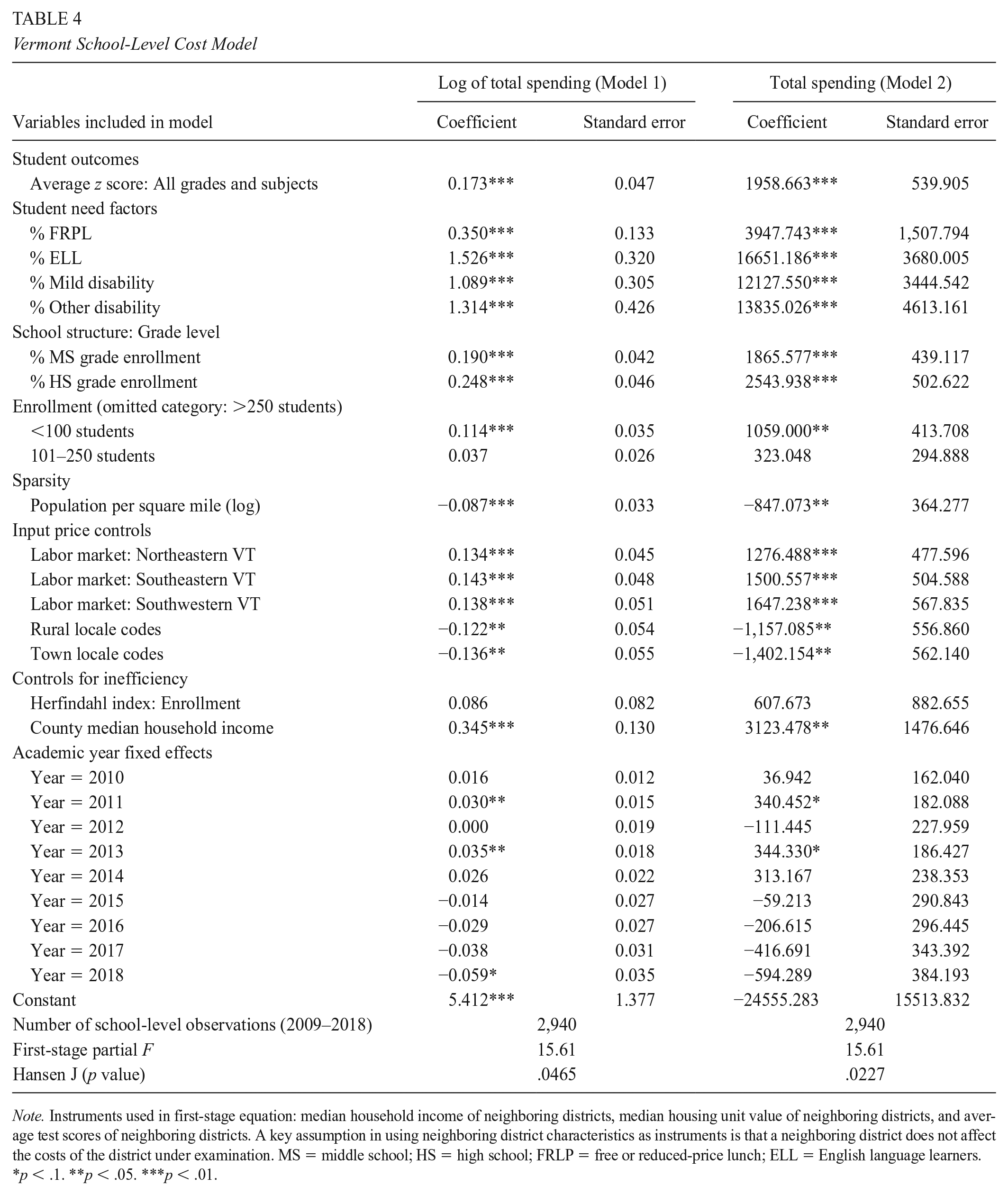
Note. Instruments used in first-stage equation: median household income of neighboring districts, median housing unit value of neighboring districts, and average test scores of neighboring districts. A key assumption in using neighboring district characteristics as instruments is that a neighboring district does not affect the costs of the district under examination. MS = middle school; HS = high school; FRLP = free or reduced-price lunch; ELL = English language learners.

p < .1. **p < .05. ***p < .01.

Overall, in Vermont schools, we find that a $1,958 increase in total spending per pupil is associated with a one standard deviation in our composite measure of student achievement in a school. Our findings also reaffirm that students with different learning needs require additional resources to attain similar levels of academic performance. Achieving the same outcome levels in a school where 100% of the children are from families who are FRPL-eligible is expected to cost $3,948 per pupil more than achieving the same outcome in a school where none of the children are FRPL eligible. By contrast, achieving the same outcome levels in a school where 100% of the students are ELL is associated with a $16,651 in additional per pupil costs. Similarly, attaining the same outcome levels in a school with 100% of the children having a mild disability is expected to cost an additional $12,128 per pupil than achieving the same outcome in a school where 0% of the children have such disabilities or impairments; the cost differential for students with all other types of disability is slightly higher, at $13,835 per pupil.

Controlling for differences across districts in student needs, we find that both economies of scale and population density are relevant cost factors. The cost of achieving the same outcome levels in a school with fewer than 100 pupils is expected to cost about $1,059 more per pupil in total spending, compared with schools with more than 250 students. Although not statistically significant at conventional levels, Vermont schools that enrolled between 101 and 250 students spent about $323 more per pupil to attain the same outcome levels than schools that enrolled more than 250. The population density of the district in which a school resides also had an independent effect on school spending. Specifically, we find that schools operating in the state’s most sparsely populated areas must spend more to attain similar outcomes. For example, the same achievement level for a school in a district with a population density of less than 50 people per square mile costs $587 more per pupil than a school that resides in a district with more than 100 people per square mile.

Estimating Weights for Policymaking

Vermont policymakers were most interested in evaluating existing pupil weights for differences in student needs and grade level and developing new weights for school size and geographic isolation, if appropriate. To support policymakers’ decision making, we took the additional step to convert the coefficients derived from the ECM to pupil weights that could be used in the state’s existing school funding formula. To do so, we estimated the relationship between the predicted per-pupil spending derived from our cost function models and six cost factors that could be used in Vermont’s current funding system structure. Specifically:

\begin{array}{l} Predicted {PPS}_{sj} = f ({Poverty}_{sj}, {ELL}_{sj}, {SWD}_{sj}, \\ Grade {Range}_{sj}, {Enrollment}_{sj}, \\ {Sparsity}_{s j}) \end{array}

(4)

where Predicted PPS is the predicted per pupil spending amount from the cost function mode for school (s) in year (j); Poverty is the percentage of economically disadvantaged students; SWD is composed of two variables that capture the share of students with (1) mild disabilities and (2) all other disabilities; Grade Range is the percentage of students in the middle (6–8) and high school (9–12) grades; Enrollment is composed of two measures of school size, <100 students and 100 to 250 students; and Sparsity is composed of three measures of population density in the district in which a school is located (<36 persons per square mile, 36–55 persons per square mile, and 55–100 persons per square mile).⁵

Vermont’s existing formula incorporates weights in the equalized pupil calculation in different ways, depending on the cost factor. The formula first applies grade-level weights and calculates a grade-level weighted ADM. To the grade-level weighted ADM, it applies the poverty weight. The ELL weight is directly applied to the number of ELL students not weighted by grade. Because the poverty weight is applied to the grade-level weighted ADM, this means that the poverty weight and the grade-level weights are multiplicative. In other words, the poverty weight counts for more in districts with more students in grades with higher grade-level weights compared with districts with fewer students in high-weight grades. Other weights (e.g., ELL) are additive, meaning that the effect of the weight does not change based on other weights.

Table 5 presents the estimated coefficients from the school-level weight estimation regression model. To account for the multiplicative nature of the poverty and grade-level weights, we modeled the poverty and grade-level weights as multiplicative by exponentiating them in a predictive model, as follows:

Table 5

School Model Regression Calculation for Weights

Cost factors	Coefficient	Standard error	Exponentiated multiplicative coefficients
Multiplicative coefficients
Poverty proportion	1.378	0.0239	3.97
% Enrolled in middle grades	0.204	0.00917	1.23
% Enrolled in secondary grades	0.186	0.00717	1.20
Constant	8.570	0.0123	5,144
Additive coefficients
Student need
ELL proportion	8126.6	433.1
% Mild disability	16208.6	484.9
% Other SWD district	11076.6	657.6
Enrollment
<100 students enrolled	1345.4	83.44
100–250 students enrolled	606.9	41.07
Sparsity
<36 Sparsity	1207.4	57.31
36–55 Sparsity	856.8	44.59
55–100 Sparsity	568.4	39.26
Number of observations	2,940

Note. Regression includes year (2009–2018) dummy variables in the multiplicative portion of model that are not shown in the table. ELL = English language learners; SWD = students with disabilities.

\begin{array}{l} P r e d i c t e d C o s t \\ P e r P u p i l = e^{(β_{0} + β_{1} P o v e r t y + \sum_{k = 2}^{3} β_{k} G r a d e R a n g e_{k} + \sum_{l = 4}^{12} β_{l} Y e a r_{l})} + \\ β_{13} E L L + β_{14} L o w S e v e r i t y S W D + \\ β_{15} H i g h S e v e r i t y S W D + \sum_{m = 16}^{17} β_{m} S i z e_{m} + \\ \sum_{n = 18}^{20} β_{n} S p a r s i t y_{n} + ε \end{array}

(5)

where Poverty is the percentage of students in poverty; Grade Range is the percentage of students in the middle (6–8) and high school (9–12) grades; Year is an indicator for the fiscal year (2008–2009 through 2017–2018); ELL is percentage of students designated as having limited English proficiency; LowSeverity is the percentage of students with low-severity disabilities; HighSeverity is percentage of students with high-severity disabilities; Size is total enrollment; Sparsity is the number of people per square mile; βs are estimated model coefficients; and ε is an independent and identically distributed error term. By modeling the predicted cost in this way, the relationship between the exponentiated portion of the equation and the predicted cost is log-linear, making it multiplicative, and the relationship between the remaining cost factors and the predicted cost is linear, making it additive. To calculate weights for the additive portion of the equation, we identified the “base” cost or the predicted cost for a school with no additional student needs, scale, or geographic-related costs, and in the lowest cost labor market. The remaining weights are then defined as each coefficient the linear cost factors divided by the base cost, respectively, as follows:

Weight = Cost Factor / Base Cost .

(6)

Table 5 also displays the exponentiated multiplicative coefficients and exponentiates the constant term which serves as a base amount that can be used to calculate pupil weights for specific cost factors. Here, the base amount is expressed as the exponentiated constant term plus an average of the year coefficients. The exponentiated coefficients for the multiplicative portion of the formula can be directly interpreted as weights and represent the additional cost as a percentage centered on 1. The exponentiated poverty coefficient of 3.97 means that students in poverty cost about 297% more than students not in poverty. In the calculations made by the state of Vermont, the grade-level coefficients remain centered on 1, whereas the poverty coefficient is centered on 0. To center the poverty coefficient on 0 rather than 1, we subtract 1 from the poverty coefficients. The additive weights were calculated by comparing the predicted spending level by the base cost—for example, the additional cost associated with operating a school with <100 students was $1,345, and the base cost was $5,144, equating to a weight of 0.26 for schools with fewer than 100 students.

Table 6 presents the final ECM-derived pupil weights for Vermont schools. Recommended weights for the share of economically disadvantaged and ELL students in a school were significantly different from those incorporated in current statute. Such differences between current and recommended weights are not entirely surprising. The existing weights predate the passage of Act 60 and when enacted in 1997, had weak, at best, connections to evidence about the additional costs of educating students with disparate learning needs (Kolbe et al., 2019). Our findings also reaffirm that cost differentials exist across grade levels and according to where a school is located. While the state’s existing formula includes a weight for secondary-level students (defined as Grades 7–12), we recommend splitting this factor into two distinct weights—one for middle-grade students (Grades 6–8) and another for secondary-level students (Grades 9–12).

Table 6

Cost Factor and Per Pupil Weights: Vermont Schools

Cost factors	Existing formula weights	ECM-derived weights
Multiplicative weights
% Poverty (centered on 0)	0.25	2.97
% Enrolled in middle grades (6–8) (centered on 1)		1.23
% Enrolled in secondary grades (9–12) (centered on 1)	1.13	1.20
Additive weights (all centered on 0)
Student need factors
% ELL	0.20	1.58
% Mild disability		3.15
% Other SWD		2.15
School enrollment
<100 students		0.26
100–250 students		0.12
Sparsity
<36 persons per square mile		0.23
36–55 persons per square mile		0.17
55–100 persons per square mile		0.11

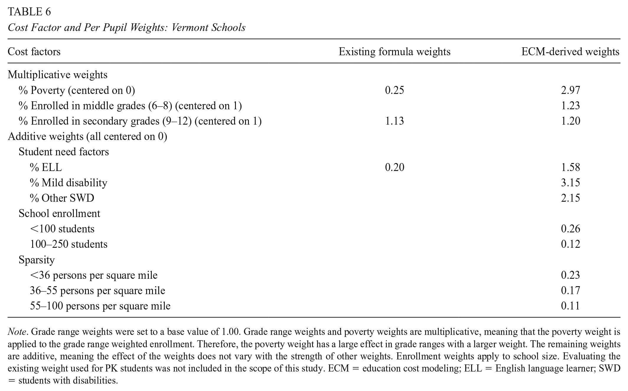
Note. Grade range weights were set to a base value of 1.00. Grade range weights and poverty weights are multiplicative, meaning that the poverty weight is applied to the grade range weighted enrollment. Therefore, the poverty weight has a large effect in grade ranges with a larger weight. The remaining weights are additive, meaning the effect of the weights does not vary with the strength of other weights. Enrollment weights apply to school size. Evaluating the existing weight used for PK students was not included in the scope of this study. ECM = education cost modeling; ELL = English language learner; SWD = students with disabilities.

We also identified weights for small schools. The per pupil weight for schools with less than 100 students was 0.26. The weight for schools with enrollment between 100 and 250 students was slightly less (0.12). This makes sense given that economies of scale might be expected to improve with increased school enrollment. Finally, weights were generated for schools located in rural areas according to the population density of the community in which a district is located. The pupil weight for schools in the state’s most sparsely populated areas, defined as having less than 36 persons per square mile, was 0.23, and like the weights for size, decreased as population density increased; 0.17 for schools located in districts with 36 to 55 persons per square mile and 0.11 for schools in districts with 55 to 100 persons per square mile.

Discussion

A key goal for state education policies has been to develop funding programs that provide additional resources to school districts that face higher costs in educating students to common standards. Ideally, state policy decisions for making cost adjustments would be set according to accurate measures of the cost of achieving a state’s goals for educational adequacy (e.g., some average level of student achievement or proficiency). Insufficient or inaccurate measures of cost differentials fundamentally undermine the ability of state operating aid formulas to ensure districts and schools have sufficient resources to provide an adequate education (Duncombe et al., 2015). Put simply, state policymakers need to know precisely how much money each district needs to meet a state’s goals for student performance. Such cost estimates assist legislators in setting spending levels consistent with outcome demands and goals that are attainable at desired spending levels. Cost estimates may also guide courts in determining whether current funding levels and distributions (or the minimum educational achievement goals, for that matter) are unreasonable, insufficient, or otherwise substantially misaligned with constitutional or other legal requirements.

In this article, we describe the approach we used in Vermont to develop a rational, empirically based policy framework for addressing cost differences for its rural schools. In doing so, we show how the state leveraged existing administrative data and applied rigorous statistical methods to estimate cost differentials for operating small schools and those located in geographically isolated areas. Our approach to estimating cost differentials for Vermont policymakers was novel, not only because district size and geographic location were explicitly considered as cost factors in the analysis but also because the effort advances knowledge about applying ECM to developing pupil weights for state K–12 school funding formulae.

In this study, we show that school size and population density, in Vermont, operate as independent cost factors, and as such, should be considered separately for the purposes of estimating cost differentials in rural schools. While, necessarily, cost differentials are state specific, due to varying preferences across states for student performance, Vermont’s findings should prompt other K–12 education finance research to explicitly consider enrollment measures and population density when estimating cost differentials across districts and schools in a state. Currently, nearly half of states include some adjustment for differences in cost across districts and schools with small enrollments, and 13 states consider district location as a cost factor. This study provides an example that states may follow to evaluate their existing policies, and for states without existing adjustments for differences in cost, how they might explore cost adjustments for small, rural schools. In Vermont, the study’s findings form the basis for proposed legislation to modify the state’s existing school funding formula. The state’s General Assembly is expected to deliberate proposed legislation during the 2021 legislative session.

We also demonstrate the utility of using ECM as an analytic approach to estimating cost differentials across schools in a state. Despite increased interest in applying ECM to estimating costs for K–12 education finance research, to date, state school funding cost studies have largely relied on input-oriented approaches to estimating cost differentials across districts and schools (Aportela et al., 2014). Such approaches have drawn criticism for the level of effort and cost in implementation, as well as methodological limitations, particularly when estimating costs for districts and schools that do not comport with the prototypes considered by professional judgment panels or evidence-based models (Baker et al., 2008). By comparison, in this study we show how grounding cost estimation in the actual experiences of schools in a state, as articulated by spending patterns, ECM is able to model spending differentials in a way that utilizes existing state data systems to provide actionable evidence state policymakers can use to develop equitable funding policies for all schools, including those with limited economies of scale and that are located in geographically remote areas.

Our work with Vermont policymakers to conduct this study also highlights several important considerations for applying similar approaches in other states. First, modeling cost differentials using ECM requires appropriate and adequate data at the district and school levels, especially measures of student performance on state assessments or for other outcomes of interest, and the ability to link these data to other indicators of community context such as median household income and population density. While many states have made great strides toward expanding and improving data infrastructure, making it now possible to apply ECM, it is also the case that analysts who pursue this approach will need to carefully consider to what extent data are sufficient to support modeling at the district or school levels and how data from state administrative databases may be linked with other extant sources (e.g., SEDA, ACS, CCD).

It is also necessary to recognize that estimates resulting from the ECM cannot account for changes in the relationship between education spending and measures of student performance that may occur in the future. In Vermont, for example, a key consideration was possible future gains in efficiency attributable to further changes in district and school governance, through consolidation, that may occur in the future. For this study, and others who may apply a similar analytic approach, this does not mean that the estimates, and resulting weights, are biased or not useful to policymakers. Rather, they are conditioned on historical spending data. Cost estimation should be periodically updated using new data, and pupil weights recalibrated as appropriate. That said, the need to recheck and potentially recalibrate cost differentials would occur regardless of whether school district consolidation transpired. Like input-based methods used in school finance research (e.g., professional judgment approach), cost differential estimation should be conducted periodically to ensure that estimated differentials best reflect current policies, educational practices, and local context in states and districts.

Finally, for this and other future studies, it will be important to carefully consider the measure(s) of student performance that are incorporated into the models. There is long-standing and lively debate about the strengths and weaknesses of different measures of student performance, and the extent to which certain measures—particularly student achievement on standardized assessments—are sufficient proxies for the types of outcomes policymakers desire from public schools. The selection of outcome measures is important for model estimation. Because efficiency is defined by the selected performance measures, the division between costs and efficiency can vary across performance measures. Accordingly, when estimating the ECM using different performance measures (e.g., value-added or student growth measures), we may not expect to have the same variation in costs across schools. In fact, it is likely that the relationship between spending and different student outcomes might be different. This is why it is necessary to select measures of student performance that are most salient for policymaking in a particular state context.

Footnotes

Appendix

Table A1

First Stage Model: Predicting Student Outcomes

Variables included in model	Coefficient	Standard error
Neighboring district median household income within supervisory union (log)^a	1.598	1.284
Neighboring district median housing value within supervisory union (log)^a	−1.631	1.280
Neighboring district test scores within supervisory union^a	0.415	0.064
Labor market: Northeastern VT	−0.208	0.161
Labor market: Southeastern VT	−0.160	0.140
Labor market: Southwestern VT	−0.239	0.141
% FRPL	−2.063	0.208
% ELL	−2.570	0.843
% Mild disability	−2.367	0.765
% Other disability	−3.195	0.929
% MS grade enrollment	−0.211	0.107
% HS grade enrollment	−0.401	0.104
<100 students	0.153	0.081
101–250 students	0.128	0.059
Rural locale codes	−0.041	0.120
Town locale codes	−0.017	0.127
Population per square mile (log)	0.042	0.091
Herfindahl index: Enrollment	−0.310	0.292
County median household Income	−0.679	0.362
Year = 2010	0.035	0.030
Year = 2011	0.141	0.036
Year = 2012	0.207	0.041
Year = 2013	0.140	0.055
Year = 2014	0.261	0.043
Year = 2015	0.295	0.062
Year = 2016	0.313	0.064
Year = 2017	0.345	0.069
Year = 2018	0.391	0.078
Constant	10.314	4.017
N	2,940
F test of excluded instruments	F(3, 302) = 15.61

Note. FRPL = free or reduced-price lunch; ELL = English language learners; MS, middle school; HS, high school.

Excluded instruments.

1.

When evaluating the appropriateness of the AOE FRPL measure, we further disaggregated the data according to the share of students who receive free lunch and those who receive reduced-price lunch.

2.

As model identification is an iterative process, we tested a variety of measures typically used to capture public monitoring (classic determinants of local demand for increased public expenditure), including the share of the population that is school aged and the share of total revenue received through intergovernmental aid. These did not prove useful in any variations of our models. We note that while our Herfindahl index does not yield a statistically significant coefficient in the model presented herein, that it did in many other intermediate variations on these models, which were collectively used to inform our final recommendations.

3.

Alternative model specifications exist for fitting second stage models to the cost frontier rather than the mean (e.g., Stochastic Frontier models and Data Envelopment Analysis. Taylor and colleagues have developed work - around methods for treating outcomes as endogenous in a Stochastic Frontier application (Gronberg et al., 2011; Taylor et al., 2018). But, to the extent that the functional form of the model when estimated by ordinary least squares, 2SLS, or stochastic frontier remains constant, or robust, then the difference in cost estimation is reflected only in the levels of predicted values across all units, and not in their variation across schools or districts.

4.

We opt to project expenditures associated with achieving a given level of outcomes assuming average rates of efficiency, that is, holding efficiency factors constant, at their average, rather than maximized or minimized efficiency. This choice is based on the difficulty associated with accurately identifying maximized efficiency across the rate of district and school types in any setting.

5.

The state defined fewer than 100 persons per square mile as a sparsely populated area. To estimate reasonable and stable differences across the population density categories each category needs a large number of schools. Using categories that have clear (whole number) cutoffs makes sense from a policy perspective, as it is easier to explain and maintain consistency from year to year, compared with creating groups with equal numbers (e.g., quintiles) but where cutoffs might be decimal places and might vary from year to year as population density changes. These groups resulted in approximately equal numbers of schools in each density category. In 2016–2017, there were 70 schools in the smallest category (≤36), 59 in the next largest category (36–55), and 66 in the 55 to 100 category. A total of 100 schools is in the >100 category.

Authors

TAMMY KOLBE is an associate professor of educational leadership and policy at the University of Vermont. Her research focuses on understanding the cost of education policies and programs.

BRUCE D. BAKER is a professor in the Department of Educational Theory, Policy, and Administration at Rutgers Graduate School of Education. His primary area of research addresses conceptions of equity, adequacy, and equal opportunity in school finance and empirical methods for estimating education cost, and cost variations by student needs and contextual factors.

DREW ATCHISON is a senior researcher at the American Institutes for Research (AIR). His primary responsibilities include quantitative analysis on a wide range of projects examining topics such as accountability, education finance, and educational equity.

JESSE LEVIN is a principal research economist at the American Institutes for Research (AIR), where he has directed projects investigating school finance equity and adequacy, resource allocation, and educational effectiveness. He currently serves as the director of several cost analysis/cost effectiveness components of randomized control trial studies for various educational interventions, and recently served as the director of a national study of district weighted student funding systems and as deputy director for a national study of Title I resource allocation, both funded by the U.S. Department of Education.

PHOEBE HARRIS is a research assistant at Child Trends Inc. She was a member of the research team as an undergraduate student in human development and family studies at the University of Vermont.

References

Andrews

Duncombe

W. D.

Yinger

(2002). Revisiting economies of size in American education: Are we any closer to a consensus? Economics of Education Review, 21(3), 245–262. https://doi.org/10.1016/S0272-7757(01)00006-1

Aportela

Picus

L. O.

Odden

Fermanich

(2014). A comprehensive review of state adequacy studies since 2003. APA Consulting. http://www.marylandpublicschools.org/Documents/adequacystudy/AdequacyReviewReport_rev_091214.pdf

Atchison

Levin

Baker

Kolbe

(2020). Equity and adequacy of New Hampshire school funding: A cost modeling approach. American Institutes for Research.

Baker

B. D.

(2006). Evaluating the reliability, validity, and usefulness of education cost studies. Journal of Education Finance, 32(2), 170–201.

Baker

B. D.

(2011). Exploring the sensitivity of education costs to racial composition of schools and race-neutral alternative measures: A cost function application to Missouri. Peabody Journal of Education, 86(1), 58–83. https://doi.org/10.1080/0161956X.2011.539957

Baker

B. D.

(2018). Educational inequality and school finance: Why money matters for America’s students. Harvard Education Press.

Baker

B. D.

Duncombe

W. D.

(2004). Balancing district needs and student needs: The role of economies of scale adjustments and pupil need weights in school finance formulas. Journal of Education Finance, 29(3), 195–221.

Chakraborty

Poggio

(2008). Efficiency and equity in school funding: A case study for Kansas. International Advances in Economic Research, 14(2), 228–241. https://doi.org/10.1007/s11294-008-9137-z

Chambers

J. G.

(1999). Measuring resources in education: From Accounting to the resource cost model approach. (Working paper No. 1999-16). U.S. Department of Education National Center for Education Statistics. https://nces.ed.gov/pubs99/199916.pdf

10.

Downes

T. A.

(2004). What is adequate? Operationalizing the concept of adequacy for New York. New York Education Finance Research Symposium. http://rockefeller.tc-library.org/Content.asp?abstract=true&uid=349

11.

Downes

T. A.

Pogue

(1994). Adjusting school aid formulas for the higher cost of educating disadvantaged students. National Tax Journal, 47(1), 89–110. https://ntanet.org/NTJ/47/1/ntj-v47n01p89-110-adjusting-school-aid-formulas.pdf?v=%CE%B1&r=5943970666266978

12.

Downes

T. A.

Stiefel

(2015). Measuring equity and adequacy in school finance. In Ladd

H. F.

Goertz

M. E.

(Eds.), Handbook of research in education finance and policy (2nd ed., pp. 244–259). Routledge.

13.

Duncombe

W. D.

Lukemeyer

Yinger

(2008). The No Child Left Behind Act: Have federal funds been left behind? Public Finance Review, 36(4), 381–407. https://doi.org/10.1177/1091142107305220

14.

Duncombe

W. D.

Nguyen-Hoang

Yinger

(2015). Measurement of cost differentials. In Ladd

H. F.

Goertz

M. E.

(Eds.), Handbook of research in education finance and policy (2nd ed., pp. 260–278). Routledge.

15.

Duncombe

W. D.

Yinger

(2000). Financing higher student performance standards: The case of New York State. Economics of Education Review, 19(4), 363–386. https://doi.org/10.1016/S0272-7757(00)00004-2

16.

Duncombe

W. D.

Yinger

(2005). How much more does a disadvantaged student cost? Economics of Education Review, 24(50), 513–532. https://doi.org/10.1016/j.econedurev.2004.07.015

17.

Duncombe

W. D.

Yinger

(2007). Does school district consolidation cut costs? Education Finance and Policy, 2(4), 341–375. https://doi.org/10.1162/edfp.2007.2.4.341

18.

Duncombe

W. D.

Yinger

(2011). Are education cost functions ready for prime time? An examination of their validity and reliability. Peabody Journal of Education, 86(1), 28–57. https://doi.org/10.1080/0161956X.2011.539953

19.

Gronberg

T. J.

Jansen

D. W.

Karakaplan

M. U.

Taylor

L. L.

(2011). The adequacy of educational cost functions: Lessons from Texas. Peabody Journal of Education, 86(1), 3–27. https://doi.org/10.1080/0161956X.2011.539953

20.

Grosskopf

Hayes

K. J.

Taylor

L. L.

Weber

W. L.

(2001). On the determinants of school district efficiency: Competition and monitoring. Journal of Urban Economics, 49(3), 453–478. https://doi.org/10.1006/juec.2000.2201

21.

Imazeki

(2008). Assessing the costs of adequacy in California public schools: A cost function approach. Education Finance and Policy, 3(1), 90–108. https://doi.org/10.1162/edfp.2008.3.1.90

22.

Imazeki

Reschovsky

(2003). Financing adequate education in rural settings. Journal of Education Finance, 29(2), 137–156.

23.

Kirkaldy

(2015, January 25). End of small school grants would hit home. Addison County Independent. https://addisonindependent.com/end-small-school-grants-would-hit-home-0

24.

Kolbe

Baker

Atchison

Levin

(2019). Study of pupil weights in Vermont’s Education Funding Formula. University of Vermont. https://legislature.vermont.gov/assets/Legislative-Reports/edu-legislative-report-pupil-weighting-factors-2019.pdf

25.

Malhoit

(2005). Providing rural students with a high quality education: The rural perspective on the concept of educational adequacy. Rural School and Community Trust. https://www.ruraledu.org/user_uploads/file/Providing_Rural_Students.pdf.

26.

Picus

L. O.

Odden

Glenn

Griffith

Wolkoff

(2012). An evaluation of Vermont’s education finance system. Picus Odden. http://picusodden.com/wp-content/uploads/2013/09/VT_Finance_Study_1-18-2012.pdf

27.

Showalter

Harman

Johnson

Klein

(2019). Why rural matters 2018-2019: The time is now. Rural School and Community Trust. http://www.ruraledu.org/WhyRuralMatters.pdf

28.

Sipple

Brent

(2015). Challenges and strategies associated with rural school settings. In Ladd

H. F.

Goertz

M. E.

(Eds.), Handbook of research in education finance and policy (2nd ed., pp. 607–622). Routledge.

29.

Strange

(2011). Finding fairness for rural students. Phi Delta Kappan, 92(6), 8–15. https://doi.org/10.1177/003172171109200603

30.

Taylor

L. L.

(2006). Comparable wages, inflation, and school finance equity. Education Finance and Policy, 1(3), 349–371. https://doi.org/10.1162/edfp.2006.1.3.349

31.

Taylor

L. L.

Fowler

W. J.

(2006). A comparable wage approach to geographic cost adjustment (NCES 2006-321). U.S. Department of Education, National Center for Education Statistics.

32.

Taylor

L. L.

Willis

Berg-Jacobson

Jaquet

Capras

(2018). Estimating the costs associated with reaching student achievement expectations for Kansas public education students: A cost function approach. WestEd.

33.

Vermont Agency of Education. (n.d.). Determining small school grants eligibility. https://education.vermont.gov/memos/state-board/determining-small-school-grants-eligibility

34.

Zimmer

DeBoer

Hirth

(2009). Examining economies of scale in school consolidation: Assessment of Indiana school districts. Journal of Education Finance, 35(2), 103–127. https://doi.org/10.1353/jef.0.0012

The Additional Cost of Operating Rural Schools: Evidence From Vermont

Abstract

Keywords

Conceptual and Empirical Background

Scale and Geographic Location as Cost Factors

Measuring Cost Differentials

Input-Oriented Analyses

Outcome-Oriented Analyses

The Vermont Policy Context

Study Design

Data

Per Pupil Spending

Student Outcomes

Student Need

School Structure

School Size

Geographic Isolation

Input Prices

Inefficiency

Analysis

Results

School-Level Model

Estimating Weights for Policymaking

Discussion

Footnotes

Appendix

1.

2.

3.

4.

5.

Authors

References