
Abstract
In the 2013–2014 school year, the state of California implemented a new equity-minded funding system, the Local Control Funding Formula (LCFF). LCFF increased minimum per-pupil funding for educationally underserved students and provided greater autonomy in allocating resources. We use the implementation of LCFF to enrich our understanding of rural school finance and explore the implications of equity-based school finance reform across urbanicity (i.e., between rural, town, suburban, and urban districts) and between rural areas of different remoteness. Drawing on 15 years of financial data from California school districts, we find variation in the funding levels of rural districts but few differences in the ways resources are allocated and only modest evidence of constrained spending in rural areas. Our results suggest that spending progressivity (i.e., spending advantage of higher-poverty districts) has increased since LCFF, although progressivity is lowest in rural districts by the end of the data panel.
In the 2013–2014 school year, the state of California overhauled its school finance system with the adoption of the Local Control Funding Formula (LCFF). The adoption of LCFF was heralded as a shift toward equity and flexibility in school funding. The formula increased funding for students considered educationally underserved (i.e., students who are any combination of English language learners [ELLs], foster youth, or eligible for free or reduced-price lunch [FRL]—referred to as “unduplicated pupils” [UPs]) and provided districts with greater autonomy in allocating resources by removing many categorical funding restrictions. These changes are thought to have had substantial benefits for students (R. C. Johnson & Tanner, 2018; Lafortune, 2019), and other states have either implemented, or are considering, similar equity-based school-funding formulas (Chingos & Blagg, 2017; Imazeki, 2018).
Yet there is little research on how schools are using the additional funds and spending discretion afforded by LCFF. In particular, there is reason to believe that LCFF may have different implications for rural districts (a third of California’s districts) than for their nonrural counterparts. Rural districts are often thought to have distinct cost structures and spending patterns due to small enrollments and geographic isolation (Hammer et al., 2005; J. Johnson & Strange, 2007; Sipple & Brent, 2015). For example, rural schools are thought to have higher expenditures and larger noninstructional expenses, although research on this issue using large-scale school finance data sets is sparse. Additionally, due to structural cost differences, rural districts may use the increased spending discretion under LCFF differently than their nonrural counterparts. Moreover, while many of the state’s rural districts serve high proportions of underserved students (National Center for Education Statistics [NCES], 2016), LCFF makes numerous exceptions to its need-based formula that may weaken the policy’s overall goal of advancing progressive school funding. For example, small districts that would have received more funding under the pre-LCFF system are exempt from some funding changes. It is therefore unclear whether rural school districts serving underserved students will enjoy the same increases in spending progressivity as other districts under LCFF.
We use the implementation of LCFF to examine three research questions:
Drawing on 15 years of detailed financial reports from California districts, we find that, contrary to conventional wisdom and some existing research, rural and nonrural districts generally allocate funds similarly. We detect the most substantial spending differences for remote rural districts, though even here the evidence is modest. Additionally, most districts experienced increases in spending progressivity (defined as the spending advantage of districts where poor students are enrolled) after the adoption of LCFF, but progressivity was not maintained for some rural districts, perhaps due to changes in other funding sources that are negatively related to student poverty (e.g., local revenues). Finally, we find only modest differences in how rural and nonrural districts have allocated new resources in the LCFF era, which may indicate that the cost disadvantages faced by rural districts are less substantial than is often assumed. These results add nuance to our understanding of district spending patterns across urbanicities, while also highlighting the ways equity-oriented funding reforms could fall short of their goals.
California’s Local Control Funding Formula
LCFF signaled a departure from a system that allocated funds based on district characteristics (viz., student enrollment and grade levels served) and numerous categorical programs to a system that allocates funds based on student characteristics and provides greater spending flexibility (Bruno, 2018; Weston, 2010). LCFF is a foundation aid formula with pupil-weighted supplemental supports. Under LCFF, in addition to a per-pupil base grant adjusted by grade level, districts receive a supplemental grant amounting to 20% of the base grant for each UP. Districts that serve more than 55% UPs receive a concentration grant for each marginal UP worth an additional 50% of the student’s base grant. However, LCFF also included several exceptions to this basic funding formula, including a “hold harmless” clause for districts that would have otherwise lost funding relative to the previous funding formula and adjustments for districts with small enrollment sizes. The state established a transition period beginning in the 2013–2014 school year to gradually meet the funding targets required by the formula, and by the 2017–2018 school year, 97% of districts’ funding targets were fulfilled (California Department of Education [CDE], 2020).
Along with changes to funding levels, districts gained discretion in how to allocate funds, because most of the categorical programs were removed under LCFF. Spending restrictions were eliminated for approximately three quarters of the existing categorical funding streams (M. Taylor, 2013). Instead, districts are expected to gather a broad group of stakeholders to develop Local Control Accountability Plans (LCAPs) that document how funds will be spent to further district goals, including how supplemental and concentration funds will be used to improve the educational outcomes of UPs.
Review of the Literature on Rural School Finance
A range of criteria have been used to identify rural districts, including geographical indicators (e.g., density, distance from urban areas) and cultural or economic traits (e.g., lifestyle, agriculture). Many studies have classified schools and districts as rural using the U.S. Census Bureau’s definition (i.e., any population, housing, or territory not in an urban area; Fan & Chen, 1999; Ward, 2003), based on proximity to a Census-defined metropolitan statistical area (Burdick-Will & Logan, 2017), or using the NCES’s school district locale codes, which are based on distance to an urban area (Sielke, 2004). The absence of a common definition makes it challenging to draw comparisons between rural school studies (Manly et al., 2019).
Few studies consider heterogeneity within the category of “rural.” As we discuss below, geographic isolation is thought to pose challenges for rural schools (e.g., fewer service providers, sparsity of enrollment). If so, more isolated rural districts would face greater challenges relative to rural districts closer to urban areas. With one exception (Burdick-Will & Logan, 2017), studies have not differentiated rural schools from one another, although NCES locale codes make this possible by distinguishing between rural districts based on their proximity to an urban area.
Cost Challenges in Rural School Districts
Existing research suggests distinct challenges in educating students in rural areas stemming from two common characteristics of rural districts: sparsity of students and geographic isolation. These factors are thought to prevent rural districts from enjoying economies of scale (Andrews et al., 2002; Duncombe & Yinger, 2007; Imerman & Otto, 2003; T. Zimmer et al., 2009). Economies of scale can be achieved in education because, to a certain extent, the quality of services provided by educators generally does not diminish as the number of students increases. For example, superintendents can typically provide similar-quality services as student enrollment grows (Duncombe & Yinger, 2007). Larger-enrollment districts can also enjoy economies because education requires physical infrastructure and maintenance (e.g., school buildings, heating systems, school buses), which cost less per pupil at scale. As a result, rural districts tend to have higher per-pupil costs because they are smaller (Andrews et al., 2002; Levin et al., 2011; Provasnik et al., 2007).
Yet economies of scale increase only up until a point, appearing to diminish or become negligible after enrollments reach roughly 4,000 (Andrews et al., 2002). Benefits of scale may even reverse for very large districts, due to transportation costs, costs associated with labor relations, and the organizational challenges of engagement and motivation in larger settings (Duncombe & Yinger, 2007). Most rural districts in California, however, have enrollments where economies of scale may still matter in important ways; while half of nonrural districts have enrollments greater than 4,000, only 6% of rural districts do.
Rural districts are thought to allocate their budgets in distinct ways from nonrural districts because of the dual challenges of isolation and sparsity. Noninstructional costs, such as those related to administration, transportation, and infrastructure, are thought to be higher in rural schools (Duncombe & Yinger, 2007; Killeen & Sipple, 2000; Showalter et al., 2017; Sipple & Brent, 2015). Spending on these higher-cost activities are thought to crowd out more student-facing expenditures in rural districts, such as those directly related to instruction and student services. Yet there is little empirical evidence that rural districts allocate resources in ways that greatly differ from those of nonrural districts, or whether those differences reflect variation in underlying cost structures (Roza, 2015). For example, while he does not consider these issues in depth, Bruno (2018) finds some differences in spending patterns between rural and nonrural districts in California in the 2016–2017 school year that are broadly consistent with the findings of the previous work discussed above. Yet these differences are mostly modest and do not point to drastically different budgetary pressures or constraints in districts of different urbanicities. Below we describe the commonly cited cost differences for rural districts in greater detail.
Transportation
Rural districts are thought to incur higher transportation costs because they have to transport students greater distances due to geographic dispersion, including transporting students to supplemental services (e.g., after-school activities) that are often at another school site (Howley, 2001; Howley et al., 2001; Killeen & Sipple, 2000; Zars, 1998). However, higher transportation costs may constitute a relatively small portion of districts’ overall budgets. For example, using a national survey of district expenditures, Killeen and Sipple (2000) found that even though per-pupil transportation spending was 50% higher in rural districts than in urban and suburban districts, these expenditures only represented roughly an additional percentage point of all spending.
Infrastructure and Capital Costs
Expenditures on building construction and maintenance are thought to be higher in rural areas because of the fixed costs involved and because smaller enrollments entail additional classroom space per student (Baker & Duncombe, 2004). As a result, rural districts are thought to spend a greater share of their budgets on covering these costs; yet the empirical evidence is lacking. In addition, rural districts have more limited access to funding for capital projects. For example, evidence from Michigan suggests that voters in rural communities are less likely to pass school facility construction bonds than those in urban and suburban areas (Bowers et al., 2010a, 2010b; R. Zimmer & Jones, 2005), perhaps because of a limited tax base that fluctuates with the price of farming commodities (Sher, 1977; Ward, 2003). Indeed, in California, rural districts tend to have lower levels of facilities funding than nonrural districts due to lower levels of local bond revenues. This is despite greater facilities funding for rural districts than for nonrural districts from the state (Brunner & Vincent, 2018). The lack of funding for infrastructure projects means that rural districts must either reallocate existing funding or delay large-scale projects until funding increases.
Teachers and Administrators
Rural districts have higher per-pupil human capital costs due to lower student-teacher and student-administrator ratios (Levin et al., 2011; Sipple & Yao, 2015; Tholkes, 1991). For instance, while Sipple and Yao (2015) find variation by state in the staffing levels of rural districts, their analysis of California, Arkansas, and Iowa finds that rural districts have higher per-pupil staffing levels than suburban districts in those states, while urban and suburban districts have similar staffing levels. School reorganization (e.g., consolidating small districts) and innovations in online learning may alleviate the financial challenges of higher per-pupil staffing. The existing evidence on the financial effects of school consolidation, however, is mixed, and there do not appear to be large-scale studies on the effects of online learning on rural school finance (Andrews et al., 2002; Brent et al., 2004; Duncombe & Yinger, 2007; Streifel et al., 1991). As such, it is unclear whether policy actions and innovations could lower per-pupil human capital costs.
Special Education and English Language Learner Services
Special education (SPED) and ELL services are thought to be more costly to deliver in rural communities, yet again, due to these districts’ smaller scale and geographic remoteness. For example, J. D. Johnson and Zoellner (2015) argue that services that require dedicated staff such as a full-time ELL teacher, SPED diagnostician, or psychologist are more costly to provide if the SPED or ELL population is not large enough to generate the funds needed to cover those costs. Lack of capacity to compete for competitive state and federal grants means that rural districts miss out on opportunities to supplement special services spending (J. Johnson & Strange, 2007). Additionally, the limited number of ancillary service providers (e.g., academic institutions with ELL and SPED specialties, professional development organizations) in rural areas complicates the delivery of services to special populations (Berry & Gravelle, 2008; Helge, 1981; J. D. Johnson & Zoellner, 2015). It is unclear to what extent these challenges shape rural school finance decisions.
Progressivity in Rural Districts
To the best of our knowledge, Provasnik et al. (2007) provide the only comparisons of funding progressivity between rural and nonrural districts using national data. Based on data from the 2003–2004 school year, the authors find that spending between low- and high-poverty districts is regressive in rural areas and progressive in urban areas. After adjusting for geographic cost differences, low-poverty rural districts spent approximately $900 more per student than high-poverty rural districts, while high-poverty urban districts spent roughly $1,100 more per student than low-poverty urban districts. These results might suggest that rural and nonrural districts could differentially benefit from states moving to equity-based funding formulas, though the authors do not distinguish between states or types of funding formula.
Contributions to the Literature
The conventional thinking among policymakers, advocates, and researchers alike is that rural districts have substantially different cost structures than their nonrural counterparts due to challenges of sparsity and geographic isolation. However, much of the existing research on rural finance is dated and does not examine whether these challenges are borne out in district spending data, reflect real cost differences as opposed to mechanical features of state funding formulas, or are moderated by school finance reforms.
Given these limitations, this article makes several contributions. First, we provide a contemporary analysis of resource allocation decisions using detailed budget data from many geographically diverse school districts. As previously mentioned, much of the existing literature on rural district spending often does not directly examine district budgets, instead speculating about spending patterns based on theoretical challenges rural districts are thought to face. Second, we examine the changes in resource allocation decisions when districts are given increased autonomy in budgeting decisions. By doing so, we can infer the areas where rural districts were cost constrained before receiving additional funding and flexibility. Third, we examine spending progressivity in light of equity-minded school finance reforms. To the best of our knowledge, there is only one study that examines differences in funding progressivity across urbanicities and no studies that examine how progressivity changes as a result of equity-based reforms like LCFF. Fourth, we disaggregate rural districts (i.e., fringe, distant, and remote rural districts) in our results to understand how varying degrees of geographic isolation are related to district spending.
Data and Analytical Approach
Data Sources
Our primary data source is annual district financial releases provided by CDE from the 2003–2004 to 2017–2018 school years. As of the 2003–2004 school year, CDE has required all local education agencies—including school districts—to submit revenue and expenditure reports every year using a “standardized account code structure,” or SACS. Local education agencies are required to classify their expenditures using numerical codes according to the goal they are trying to accomplish, the activity by which that goal is being accomplished, and the object (i.e., the good or service) being purchased. To streamline analysis, we combine closely related codes to generate broad categories of expenditures (CDE, 2016). These code combinations are discussed in more detail below.
We supplement these SACS data with other publicly available data from CDE, NCES, and the U.S. Census Bureau. Specifically, we draw on CDE’s Current Expense of Education reports, which include average daily attendance (ADA) figures for districts. 1 District characteristics and student demographics are obtained from CDE and NCES’ School and District Universe Surveys. NCES locale codes are used to identify the urbanicity of school districts by their size and proximity to an urbanized area (i.e., a densely settled core with densely settled surrounding areas). 2 These codes classify districts broadly as rural (located in a nonurban territory), city (located within a principal city of a metropolitan area), suburban (located in an urban area but outside the boundary of a principal city), and town (located in an urban cluster 3 ). Because the challenges to rural school finance are thought to be related to geographic isolation, we further disaggregate the rural category into rural fringe districts (rural territories no more than 5 miles from an urbanized area or 2.5 miles from an urban cluster), rural distant districts (rural territories 5–25 miles from an urbanized area or 2.5–10 miles from an urban cluster), and rural remote districts (rural territories more than 25 miles from an urbanized area and more than 10 miles from an urban cluster). Finally, we generate district poverty figures for children aged 5 to 17 years from the Census Bureau’s Model-Based Small-Area Income and Poverty Estimates.
Expenditure Measures
We make use of the detailed SACS data by constructing several measures of district spending. A few factors complicate the process of constructing district expenditure measures, and we describe these in greater detail in Appendix A (see the online version of this journal). Along with aggregating all expenditures into a total expenditure measure, it is often conceptually useful to distinguish between a district’s spending for day-to-day educational services to its K–12 students—sometimes referred to as “operational” spending—and spending on costs that are relatively fixed or indirectly related to K–12 education. As in previous work (Bruno, 2018; Loeb et al., 2007), we draw a distinction between “student” spending and “nonstudent” spending by classifying expenditures as “nonstudent” if they are for pre-kindergarten or adult education, capital costs (except equipment replacement), debt service, retiree benefits, or services to other agencies or to the community. Our measure of student spending is simply a subset of total expenditures, excluding nonstudent spending, that is focused on districts’ day-to-day operational expenditures for its K–12 educational programs. 4 Thus, the student and nonstudent categories are mutually exclusive and collectively include all district expenditures. The transactions excluded in student spending are summarized in Table 1. We also examine a few expenditures in greater detail. These include expenditures related to specific activities and objects, such as instruction, student services, transportation, administration, plant services (i.e., building and maintenance), capital outlay, salaries, and benefits. 5
Transactions Excluded From Student Expenditures

Note. SACS = standardized account code structure; PERS = Public Employees’ Retirement System.
Equipment replacement (Object Code 6500) is included in student spending.
To facilitate comparison across years, financial figures are inflation adjusted and expressed in 2018 dollars. Additionally, all spending measures are weighted by ADA. Doing so captures the experience of the typical student rather than the typical district. This decision has implications for the size of spending differences between rural and nonrural districts, but it has little bearing on resource allocation differences within rural and nonrural districts. In all cases, ADA-weighted figures are smaller than their unweighted counterparts (see the online Appendix Table A2). This is not entirely surprising because districts with larger enrollments also tend to spend less per pupil.
District Sample
Table 2 includes summary statistics related to district demographics and spending measures for the 2012–2013 school year (the year before LCFF was implemented) disaggregated by locale. While more than a third of California districts are rural, the vast majority of students (roughly 90%) are enrolled in cities and suburbs. Approximately 6% of students are enrolled in towns, with 4% enrolled in rural districts. As seen in Table 2, average district size increases as we move from rural to urban districts, though there is considerable variation, including some very small enrollments, in all locales. 6 Rural districts enroll similar shares of FRL students when compared with other districts, and in the case of rural remote districts, they enroll higher shares of FRL students than urban districts. Rural and town districts enroll fewer students of color than suburban and urban districts, and they enroll fewer ELLs than urban districts. Table 2 suggests variation in spending patterns within and between locales, with remote rural districts spending the most per ADA. We examine these spending categories in greater detail in the next section.
District Summary Statistics by Locale, 2012–2013 School Year
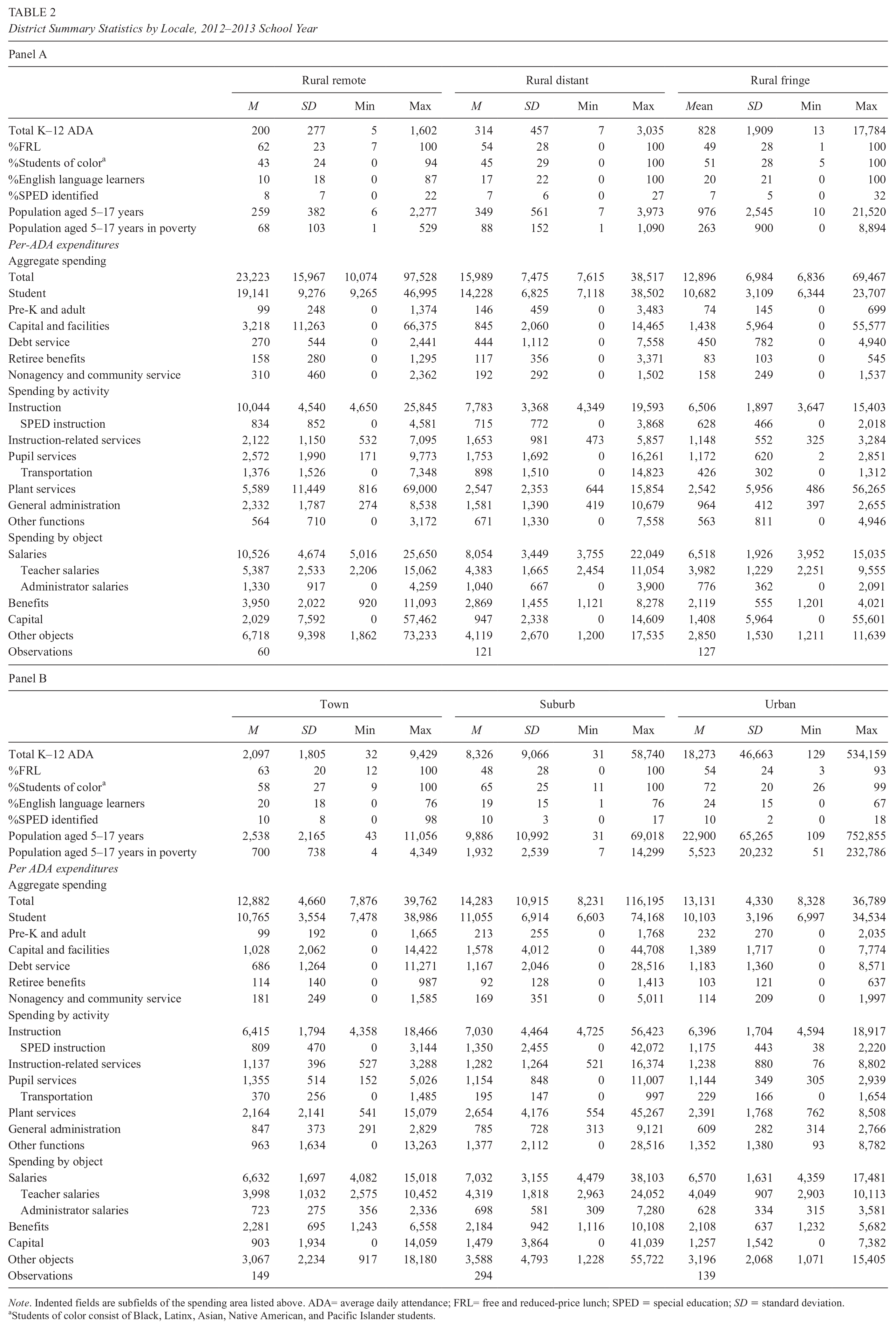
Note. Indented fields are subfields of the spending area listed above. ADA= average daily attendance; FRL= free and reduced-price lunch; SPED = special education; SD = standard deviation.
Students of color consist of Black, Latinx, Asian, Native American, and Pacific Islander students.
Analytical Approach
We use a combination of summary statistics and descriptive data techniques to answer our research questions. Beginning with Research Question 1 (level and share of spending post-LCFF), we regress raw spending and the share of each spending category for the 2017–2018 school year on a set of dummy indicators for each locale (rural distant, rural fringe, town, suburb, urban) with rural remote serving as the reference category. The constant from these models provides the spending level (or share) for rural remote districts, and the coefficients show how much each locale differs from rural remote districts. The same regression technique is used for Research Question 3 (changes in spending post-LCFF). That is, we regress the raw difference and percent change in spending between pre-LCFF (2012–2013 school year) and post-LCFF (2017–2018 school year) on the same locale indicators as described above.7,8All regressions are weighted for ADA, and standard errors are robust to heteroskedasticity.
For Research Question 2 (resource gaps and progressivity under LCFF), we graph trends in total and student spending by locale over the course of the data panel. We also construct a statewide measure of spending progressivity—similar to the one developed by Chingos and Blagg (2017)—by locale. For each locale, we calculate a weighted average of per-pupil student spending, where the weight is the number of children 5 to 17 years old who are in poverty in a given district. We then calculate a second pair of averages where the weight is the number of children 5 to 17 years old who are not in poverty. The progressivity for each group of districts by locale (e.g., rural districts) is the difference between their poverty-weighted and non-poverty-weighted means. The measure describes whether poor students are enrolled in districts with higher or lower spending levels than the districts in which nonpoor students are enrolled. 9
Findings
Research Question 1: How Do the Level and Distribution of Expenditures Vary Between Rural and Nonrural Districts in California?
As discussed above, rural district spending patterns are thought to differ from those in nonrural districts in a few key ways, including higher per-pupil spending, a smaller share of the budget allocated to student spending, and a greater share allocated to other indirect expenses (e.g., transportation, infrastructure, and capital costs). We examine whether these differences are apparent in school finance data from the 2017–2018 school year (i.e., after LCFF was implemented).
Table 3 displays the regression results for total, student, and nonstudent spending levels and shares by locale. Our results suggest differences in overall spending levels, though primarily for remote rural districts. As seen in Table 3, column 1, consistent with previous literature, remote rural districts spend $22,665 per pupil overall, but other rural districts spend considerably less—much closer to spending in nonrural districts. For example, total per-pupil expenditures in distant rural districts are $5,136 lower than in remote districts (albeit only marginally significantly), while fringe districts spend $7,643 less. From a total expenditure perspective, fringe and distant districts are much more similar to urban, suburban, and town districts than to remote rural districts.
Per-ADA Total, Student, and Nonstudent Expenditure Levels and Shares, 2017–2018

Note. Robust standard errors are in parentheses. ADA weighted and expressed in 2018 dollars. Each column constitutes a separate regression with indicators for rural distant, rural fringe, town, suburban, and urban districts. Rural remote districts are the reference category, and the constant provides the spending level or share for these districts. Italicized text indicates subcategories of nonstudent spending. Nonstudent spending categories are not mutually exclusive and may sum to slightly more than total nonstudent spending figures. All regressions include 890 observations. ADA= average daily attendance.
p < .10. *p < .05. **p < .01. ***p < .001.
A common concern is that rural districts may be forced to dedicate expenditures disproportionately to activities that benefit students’ instructional experiences only indirectly (i.e., nonstudent spending), if at all, because they lack economies of scale and advantages of geography enjoyed by other districts. We find differences in the levels of student and nonstudent spending (which are expected given that remote rural districts outspend other districts), but they do not equate to differences in the share of resources allocated to these areas. For example, student (capital) spending accounts for almost 82% (13%) of all spending in remote rural districts, and differences in spending with other districts are never statistically significant (see Table 3, columns 9 and 11). Nor do we find consistent evidence that more isolated rural districts allocate larger shares of their budgets to “fixed” costs than other districts. In fact, in some cases, rural remote districts seem to allocate less of their budgets to these costs (e.g., debt service; see Table 3, column 12).
Spending by Activity
More specific than aggregate spending are the activity codes that are used to categorize district expenditures. Table 4 displays the differences in activity-specific spending levels and spending shares by locale. Here we find evidence of modest differences between districts that are consistent with the literature. For example, all types of nonrural districts (including cities, towns, and suburbs) allocate fewer dollars and a smaller share of their budgets to transportation ($230 to $691 less, 1.8–2.8 percentage points less) and general administration (e.g., auditing services and board of education costs; $386 to $1,025 less, 2.1–3.9 percentage points less) than remote rural districts (see Table 4, columns 5, 7, 13, and 15). Additionally, as seen in columns 6 and 14, remote rural districts spend more in terms of both spending level and share of budget on plant service costs than all other districts ($3,000 to $4,000 more, 4.2–7.7 percentage points more), although the differences are not statistically significant at conventional levels.
Per-ADA Expenditure Level and Share by Activity, 2017–2018

Note. Robust standard errors are in parentheses. ADA weighted and expressed in 2018 dollars. Each column constitutes a separate regression with indicators for rural distant, rural fringe, town, suburban, and urban districts. Rural remote districts are the reference category, and the constant provides the spending level or share for these districts. Italicized text indicates subcategories: SPED instruction is a subcategory of instruction, and transportation is a subcategory of pupil services. “Other activities” includes ancillary services, community services, enterprise, and other outgoing activities. Percentages may not add up to 100 due to rounding. All regressions include 890 observations. ADA= average daily attendance; SPED = special education.
p < .10. *p < .05. **p < .01. ***p < .001.
The fact that remote districts spend more than other districts on these activities means that they tend to allocate smaller shares of their budgets to regular instructional activities, and this is qualitatively what we see in Table 4, column 9. Remote districts spend less than 45% of their budgets on regular instruction, 3.3 to 7.1 percentage points less than districts of other urbanicities (though these differences are only statistically significant for suburban and rural fringe districts). We find similar patterns when examining SPED instruction (column 10). Of note, we find that at times rural distant and fringe allocations appear more like those of remote districts (e.g., transportation and general administration) and in other areas their spending is more similar to that of nonrural districts (e.g., instruction), which again suggests heterogeneity within rural groups.
Spending by Object
Because SACS object codes identify the goods and services districts purchase, they can further illuminate district cost structures. Table 5 displays the differences in object-specific spending by locale. All other districts spend less than remote rural districts on salaries overall ($1,199 to $1,982 less; column 1)—including teacher salaries ($140 to $550 less, although only statistically significant for towns; column 2) and administrator salaries ($186 to $481 less; column 3)—and benefits ($756 to $1,249 less; column 4). These expenditure levels, however, only sometimes translate to remote districts spending a smaller share of their budgets in these areas, which is especially the case for teacher salaries (column 8). We find few other differences between remote rural districts and other districts in how budgets are allocated by object.
Per-ADA Expenditure Level and Share by Object, 2017–2018

Note. Robust standard errors are in parentheses. ADA weighted and expressed in 2018 dollars. Each column constitutes a separate regression with indicators for rural distant, rural fringe, town, suburban, and urban districts. Rural remote districts are the reference category, and the constant provides the spending level or share for these districts. Italicized text indicates the subcategories of salaries. “Other objects” includes other operating expenditures, books and supplies, and other outgoing objects. Percentages may not add up to 100 due to rounding. All regressions include 890 observations. ADA= average daily attendance.
p < .10. *p < .05. **p < .01. ***p < .001.
In sum, we find some variation in spending consistent with what is suggested by the literature review, including differences in spending on capital, transportation, plant services, general administration, and salaries. However, contrary to expectation, these differences generally do not equate to large differences in how resources get allocated except, at times, in the most remote rural districts. Moreover, across all of the regression results reported (including those in other parts of this study), we find that the locale indicators explain little of the variance in expenditures, which supports our general conclusion that geographic locales do not explain much of the spending differences we observe. The discussion section examines possible reasons why rural and nonrural allocations are often more similar than might be expected. 10
Research Question 2: Have School-Funding Gaps and Spending Progressivity Changed Between Rural and Nonrural Districts Under LCFF?
LCFF funding rules explicitly target additional resources toward districts with larger shares of underserved students (i.e., UPs). Rural and nonrural districts educate similar shares of educationally underserved students. However, because California also carves out several exceptions to the LCFF for districts based on their size or previous funding levels and preserves potentially important roles for local revenue sources excluded from the formula, districts with similar student demographics may be differentially affected by the reform. It is therefore worth exploring whether resource levels and resource gaps between districts have changed under LCFF.
We begin by examining whether the relationship between UP shares and resource levels varies by locale. In 2017–2018, UP percent (UPP) and student spending had the strongest correlations for urban districts (r = .49), followed by weaker correlations for rural remote districts and suburban districts (r = .22–.23) and the weakest correlations for districts in towns, and both rural fringe and distant locales (r = .04–.10). 11 Thus under LCFF, while urban districts with high UPP have higher per-pupil spending than their more advantaged counterparts, the same may not be the case in rural districts.
Though we do not find large spending differences between rural and nonrural districts in 2017–2018, the fact that district spending levels are differentially related to UPP suggests that LCFF may have changed the relative spending levels of rural and nonrural districts over time. Figure 1 suggests that this is not the case. The top panel of Figure 1 shows total spending trends, and the bottom panel shows student spending trends. For all the years SACS data are available, remote rural districts have had higher total and student spending than both nonrural districts and other rural districts. Meanwhile, nonrural, rural fringe, and rural distant districts have had similar levels of total and student spending during this time. The spending gaps between remote rural districts and other districts have remained generally consistent over time. In the LCFF era, all districts have seen their spending levels rise, although remote rural districts seem to have experienced larger increases in total spending. 12

Total spending (top panel) and student spending (bottom panel) per ADA.
If LCFF has increased funding for all districts but spending levels are correlated with underserved student enrollment to varying degrees, has this had a differential influence on spending progressivity across districts? We examine progressivity trends by locale in Figure 2. For ease of visualization, we combine the similar progressivity trends of town and suburban districts. The dark black line at zero represents the dividing line between progressive and regressive spending (i.e., between higher and lower average spending in districts attended by poor students). Trends for rural districts in some cases fluctuate substantially due to smaller numbers of districts in each rural group and smaller enrollments in each district, which is especially true for remote rural districts. Nevertheless, Figure 2 suggests that progressivity differs across urbanicity and not all districts maintained progressivity under LCFF. Urban districts have had more progressive spending than most other districts (including rural ones in several instances) across the panel. Consistent with the gradual phase-in of LCFF funds, both rural and nonrural districts experienced increases in progressivity after the adoption of LCFF (with the exception of remote districts), which peaked in the 2016–2017 school year. By the end of the panel, fringe and remote rural districts experience dramatic declines that result in substantially less progressive or even regressive spending. The initial success of LCFF in advancing its stated goal of progressive spending may not be sustained in general or for some rural districts in particular. Declines in progressivity in the 2017–2018 school year may be due to other funding sources such as local revenues, which tend to be negatively related to student disadvantage in California (Bruno, 2018). Regardless, progressivity declines should be cautiously interpreted until additional years of data are available. 13

Progressivity in student spending.
Research Question 3: Are Rural and Nonrural Districts Spending New LCFF Money Differently?
Constraints on spending that dictate how districts allocate resources (e.g., spending restrictions on revenues, collective-bargaining agreements) make it challenging to detect differences in costs related to urbanicity because districts do not have complete discretion in allocating dollars toward their highest-cost or more important activities. But during the LCFF era, districts saw large increases in their spending flexibility. Under LCFF, operational funding increases were combined with the elimination of spending restrictions associated with approximately three quarters of existing categorical funding streams (M. Taylor, 2013). Consequently, between 2012–2013 and 2016–2017, not only did districts’ real per-pupil operational revenues increase by roughly 30%, but the proportion of that revenue that was restricted in how it could be spent also fell from about one quarter to about one fifth (Bruno, 2018). Comparing spending before and after the adoption of LCFF sheds light on how districts shift funding patterns when they have the flexibility to do so and may uncover areas where they were previously constrained.14,15
In Tables 6 to 8 we consider whether increases in overall funding are accompanied by similar changes in specific types of expenditures. We do so by comparing expenditures (per ADA) in 2017–2018 with their levels in 2012–2013, the last year before the implementation of LCFF. For each expenditure category, we show the difference in dollars spent between 2017–2018 and 2012–2013 (top panel) and the change in spending in 2017–2018 as a percentage of spending in 2012–2013 (bottom panel). 16 As shown in Table 6, column 1, spending increased substantially over that time period: ranging from 25% to 30% for rural and nonrural districts. In line with our previous regression results, we again find that little of the variance in expenditure changes is explained by locale.
Changes in per-ADA Expenditures in Total, Student, and Nonstudent Spending, 2012–2013 to 2017–2018
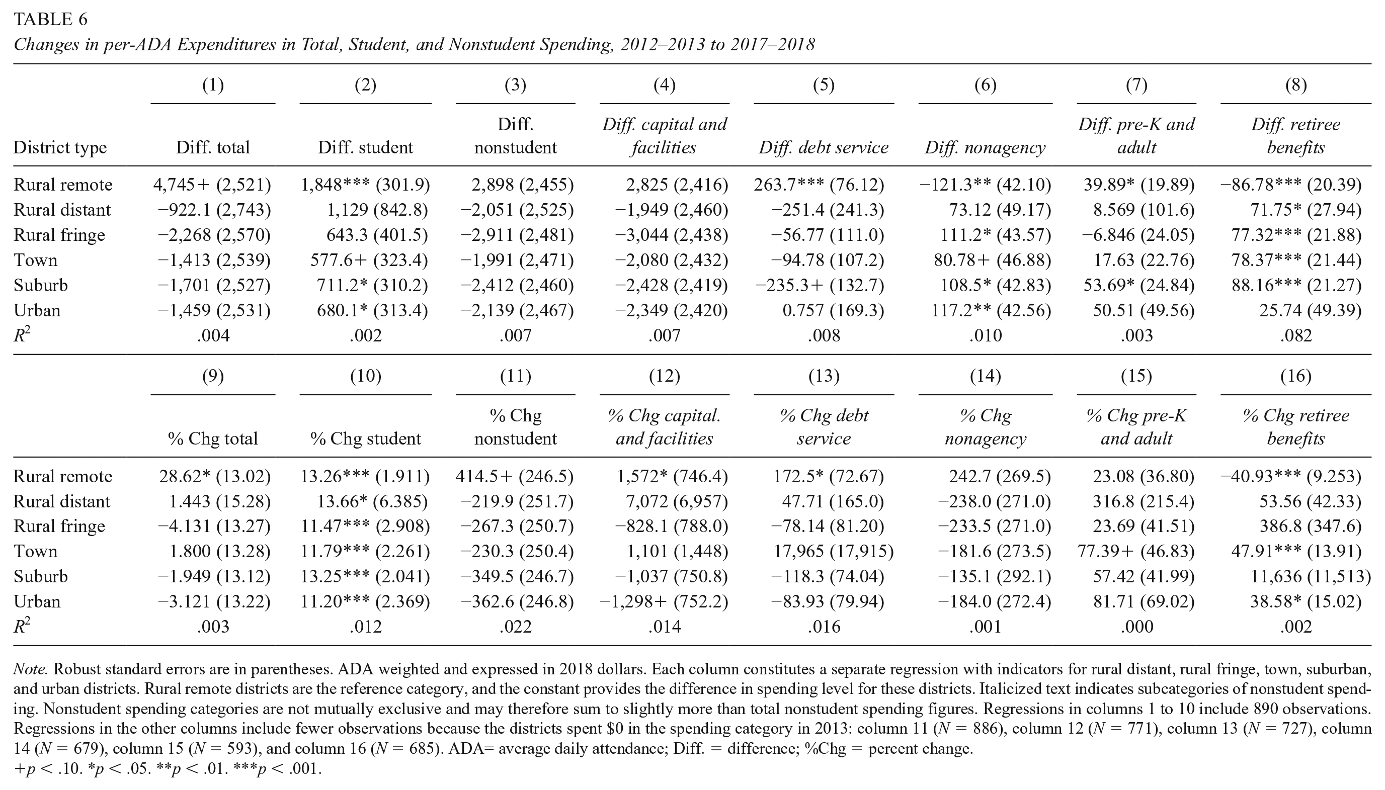
Note. Robust standard errors are in parentheses. ADA weighted and expressed in 2018 dollars. Each column constitutes a separate regression with indicators for rural distant, rural fringe, town, suburban, and urban districts. Rural remote districts are the reference category, and the constant provides the difference in spending level for these districts. Italicized text indicates subcategories of nonstudent spending. Nonstudent spending categories are not mutually exclusive and may therefore sum to slightly more than total nonstudent spending figures. Regressions in columns 1 to 10 include 890 observations. Regressions in the other columns include fewer observations because the districts spent $0 in the spending category in 2013: column 11 (N = 886), column 12 (N = 771), column 13 (N = 727), column 14 (N = 679), column 15 (N = 593), and column 16 (N = 685). ADA= average daily attendance; Diff. = difference; %Chg = percent change.
p < .10. *p < .05. **p < .01. ***p < .001.
Changes in per-ADA Expenditures by Activity, 2012–2013 to 2017–2018

Note. Robust standard errors are in parentheses. ADA weighted and expressed in 2018 dollars. Each column constitutes a separate regression with indicators for rural distant, rural fringe, town, suburban, and urban districts. Rural remote districts are the reference category, and the constant provides the difference in spending level for these districts. Italicized text indicates subcategories: SPED instruction is a subcategory of instruction, and transportation is a subcategory of pupil services. “Other activities” includes ancillary services, community services, enterprise, and other outgoing activities. Regressions in columns 1 to 9, 11, 14, and 15 include 890 observations. Regressions in the other columns include fewer observations because the districts spent $0 in the spending category in 2013: column 10 (N = 812), column 12 (N = 887), column 13 (N = 840), and column 16 (N = 823). ADA= average daily attendance; SPED = special education; Diff. = difference; % Chg = percent change.
p < .10. *p < .05. **p < .01. ***p < .001.
Changes in per-ADA Expenditures by Object, 2012–2013 to 2017–2018

Note. Robust standard errors are in parentheses. ADA weighted and expressed in 2018 dollars. Each column constitutes a separate regression with indicators for rural distant, rural fringe, town, suburban, and urban districts. Rural remote districts are the reference category, and the constant provides the difference in spending level for these districts. Italicized text indicates subcategories of salaries. “Other objects” includes other operating expenditures, books and supplies, and other outgoing objects. Regressions in columns 1 to 8, 10, and 12 include 890 observations. Regressions in the other columns include fewer observations because the districts spent $0 in the spending category in 2013: column 9 (N = 884) and column 11 (N = 766). ADA= average daily attendance; Diff. = difference; % Chg = percent change.
p < .10. *p < .05. **p < .01. ***p < .001.
Since the adoption of LCFF, both rural and nonrural districts have increased spending in many categories. In some cases, rural districts have generated larger spending increases in areas where they may have had little capacity to do so pre-LCFF. For instance, as shown in Table 6, many districts seem to have experienced the most substantial increases in nonstudent spending activities (columns 3 and 11). Remote rural districts spent almost $3,000 more in this area, which results in a roughly 400% increase in nonstudent spending. While the coefficients for other districts are not statistically significant, they are consistently negative, suggesting smaller increases in other districts. A closer examination of nonstudent spending reveals that post-LCFF, remote rural districts spend substantially more on capital and facilities and debt service than before the policy (see Table 6, columns 12 and 13). 17 To some extent, capital and facilities spending and debt service should be correlated since larger capital investments may require financing and interest payments to lenders. These activities may be particularly difficult for districts to finance in leaner budgetary times. Remote rural districts increase student spending by relatively little when compared with all other districts (Table 6, column 10), perhaps because remote districts increase nonstudent spending to a greater degree. Remote rural districts’ greater increases in nonstudent spending than in student spending (both overall and relative to what is observed for other districts) is plausibly the opposite of what we would expect if these districts have been uniquely constrained by fixed or noninstructional costs prior to LCFF. That is, theoretical arguments and conventional wisdom would suggest that rural districts would spend more on day-to-day instructional activities when given additional funds and flexibility. However, we find that even remote rural districts do not appear to invest more in this kind of student spending when given the opportunity to do so by more unrestricted revenue.
When examining spending by activities and objects, we again find that many of the differences we detect are not obviously consistent with the conventional wisdom about rural districts. For example, if fixed overhead costs crowd out instructional investments in rural districts, then rural districts should invest new funds disproportionately in instruction. In Table 7, we find that remote rural districts increase the number of dollars spent in instruction (including SPED instruction), instruction-related services, and pupil services relative to their spending prior to LCFF. Yet both other rural districts and nonrural districts increase spending by a greater amount when compared with previous spending, and they also experience greater percent change in spending (see columns 1–4 and columns 9–12). Rather than instruction, remote rural districts seem to experience their proportionally largest increases in plant services (although differences with other districts are not statistically significant; see column 14). Nonrural districts (and often rural fringe districts) experience greater spending increases than rural remote districts in areas such as salaries (particularly teachers’ salaries) and benefits (see Table 8, columns 6, 7, and 9). 18
Overall, despite the challenges described in previous literature, our results show few instances where there is evidence of unique constraints that are specific to remote rural districts or even other rural districts. If unique cost pressures substantially constrained budgets in rural districts after the recession, that is not clearly evident in unique spending patterns as revenue recovered. Rather, our results suggest more commonalities than differences in spending changes across rural and nonrural geographies. 19
Discussion and Implications
California’s LCFF is one of many recent equity-minded state education funding reforms (Chingos & Blagg, 2017; Imazeki, 2018). We contribute to the existing literature by (a) examining how spending levels and allocations differ by geography; (b) showing how spending changed by geography before and after LCFF implementation, including how progressivity has shifted for each locale; and (c) generating suggestive evidence of where rural and nonrural districts were (and were not) cost constrained in the years before the revenue increases introduced by LCFF.
Our results call into question some of the conventional wisdom around rural school finance. Despite the conventional wisdom that rural districts may have to allocate funds differently due to challenges of sparsity and scale, we find that rural and nonrural districts generally allocate funds similarly. For example, we find only modest evidence that the most isolated and smallest rural districts (remote rural districts) allocate more dollars than other districts to noninstructional expenses (e.g., transportation, general administration), and similarly modest evidence that remote rural districts are differentially cost constrained when expenditures of new, unrestricted revenues in the LCFF era are considered. The few differences we find suggest that remote rural districts are distinct from other rural districts (distant and fringe), whose budgets more closely resemble those of nonrural districts. Additionally, under LCFF, we find little evidence that spending differences between rural and nonrural districts have changed. In terms of spending progressivity, most districts experienced increases in progressivity after the adoption of LCFF. But by the end of the panel, some rural districts had returned to regressive or near-regressive spending, perhaps due to other funding sources, such as local revenues, that may be negatively related to student poverty. However, given the fluctuations in progressivity for rural districts, additional years of data will be useful in revealing whether maintaining progressivity under equity-minded school finance reform is more difficult in rural locales.
In many ways, our findings complicate the existing literature and practice that emphasize different cost structures of rural and nonrural districts. As in much other research on rural school finance, we only observe expenditures and cannot observe costs directly. We attempt to get around this challenge to some extent by examining how districts spend new money when their total revenues increase and categorical restrictions are removed. The fact that we find rural and nonrural districts spend similarly before LCFF and continue to do so when they get additional funds (and discretion) is suggestive evidence that rural and nonrural districts face similar cost constraints or otherwise have similar priorities for how to spend additional dollars. Additionally, while we often use geographic classifications like “rural” as a shorthand, our results show that very little of the variance in our outcomes is explained by locale indicators. These labels tell us very little about district expenditure patterns. This serves as a reminder to be specific in our language when referring to locale-specific challenges or opportunities in school finance.
The apparent similarity between their cost structures does not preclude rural and nonrural districts from differing in the challenges they face, such as unequal access to skilled and certificated labor. It should also be noted that there is an important distinction between level of expenditures (inputs) and quality of services or student achievement (outputs). This article focuses strictly on the former, so our results provide no information about the quality of education provided to rural students. In a study that considers spending and student achievement, Roza (2015) finds evidence that remote rural districts are overrepresented among high-achieving districts (after adjusting for student demographics) that spend at or below the state average. At a time when education leaders are bracing for future budget cuts, other districts could learn from how rural districts are stretching their dollars.
Another way to understand these findings is that rural districts do in fact face substantial cost disadvantages related to geography but they have been able to overcome these challenges through innovation, such as creating district cooperatives (e.g., educational service agencies) to achieve economies of scale and/or taking advantage of technologies (e.g., virtual schools) to decrease costs. To the extent that the similarities reflect efficiency innovations in rural districts, policymakers and administrators should try to learn from rural districts (Roza, 2015).
Implications for Policy, Practice, and Future Research
The similarities we detect between rural and nonrural areas have implications for policy and practice. State school finance systems often incorporate various kinds of supplemental funding to deal with issues of scale and sparsity, which are assumed to affect cost structures in rural districts (Kolbe et al., 2020). Adjustments made to funding formulas for rural districts seem defensible in the abstract, but it is unclear how well or how poorly these adjustments reflect the actual needs of rural districts. At the same time, states are less likely to adjust for costs that might be lower for rural districts, such as labor costs (e.g., comparable wage adjustments; Kolbe et al., 2020). The similarities in expenditures between rural and all types of nonrural districts may suggest that the rural district cost disadvantages are offset by cost advantages in some input costs (e.g., lower labor costs; L. L. Taylor & Fowler, 2006). As a result, state funding formulas may want to take both cost advantages and disadvantages into consideration. Relatedly, because rural and nonrural districts seem to spend new money similarly, our research also suggests that when states provide scarcity or sparsity adjustments within their funding systems, it may be better to make those adjustments to unrestricted revenue, where districts can decide how to spend funds, than to a categorical grant (e.g., that districts have to use for transportation).
Initial findings on how LCFF has affected rural and nonrural districts raise some questions about the progressivity of the policy. LCFF was relatively successful in raising progressivity in the first few years of its implementation, which suggests that exceptions to the funding formula did not entirely preclude progressivity gains. It remains to be seen if progressivity will continue to fall (as we see at the end of our panel) or return to previous levels. Failing to sustain progressivity could illustrate the difficulty in implementing equity-based funding at the state level when districts differ in their ability to raise local revenues. Our results may suggest that there are larger disparities in the ability to raise local funds between high- and low-poverty districts in some rural areas, although future research is needed to explore whether this is the case. If these differences between locales do exist, equity-oriented school finance reform should consider student demographics and location-specific challenges to raising local revenues simultaneously when disbursing funding to districts. Doing otherwise may penalize high-poverty rural districts and may fail to alleviate, or even exacerbate, spending inequities between rural districts.
In light of our results, further analysis, including qualitative research in rural school systems, is needed to understand how rural districts may overcome their structural financial disadvantages. For example, it could be fruitful to conduct a series of mixed-methods district case studies of rural districts or districts of varied urbanicities. In particular, selecting school systems that are positive “outliers” as mixed-methods case studies, as in Roza (2015), could generate insights into what practices rural districts with high academic gains relative to their spending (after adjusting for student demographics) are engaging in. A case study approach would facilitate the collection of more detailed quantitative data on district resource allocation than are typically available in district-level data sets (e.g., contracts with local service providers, details of regional financial arrangements between smaller districts, or draft school board budgeting documents). While it is likely difficult to generalize from these financial data, they could be interpreted with the aid of rich qualitative evidence, which is often missing in school finance literature (e.g., interviews with finance officials or observations of school board meetings). Such work could help make sense of, and reconcile, existing, larger-scale school finance studies—for example, by shedding light on the actual quality of services provided to students in rural and nonrural communities. In the case of LCFF, a case study approach could also illuminate how districts are spending LCFF funds and the extent to which targeted resources under LCFF are reaching the intended students.
While we find that locale tells us very little about school expenditures, future research should also examine whether there are other important predictors of rural expenditure patterns—for instance, whether district characteristics such as small size and geographic isolation are related to expenditure patterns. It may also be worthwhile to examine if there are other, more salient district characteristics that suggest structural cost differences. Identifying these predictors could help policymakers create funding formulas that account for the cost challenges or opportunities facing districts.
Our results also point to the importance of evaluating the implications of equity-oriented school finance reforms, not only on the basis of their “main” school-funding formulas but also inclusive of their various exceptions and “hold harmless” provisions (e.g., provisions guaranteeing that districts will not lose funding for enrollment declines or relative to the prereform funding system). Finally, school finance analyses are constrained by the specificity of reported spending. Moving forward, school-level financial data and the analysis of other LCFF-related documents, such as the LCAP, may provide a richer source of information for how and where districts are allocating funds.
Supplemental Material
sj-pdf-1-ero-10.1177_2332858420982549 – Supplemental material for The Rural/Nonrural Divide? K–12 District Spending and Implications of Equity-Based School Funding
Supplemental material, sj-pdf-1-ero-10.1177_2332858420982549 for The Rural/Nonrural Divide? K–12 District Spending and Implications of Equity-Based School Funding by Tasminda K. Dhaliwal and Paul Bruno in AERA Open
Footnotes
1.
ADA is highly correlated with point-in-time measures of school enrollment provided by NCES (r = .99). We use ADA because it is used to determine funding.
2.
NCES locale codes were updated in 2005 and 2006 to reflect both changes in the U.S. population and key geographic concepts (Geverdt, 2015). As a result, we use the codes from the earliest available year (2006–2007) for the 2003–2004, 2004–2005, and 2005–2006 school years.
3.
Urban clusters are defined as areas that contain at least 2,500 and less than 50,000 people.
4.
This definition of student spending approximately parallels the definition used by CDE to construct its “current expense of education” measure.
5.
We do not include an analysis of expenditures by goals because rural remote districts classify a much larger share of their expenditures as belonging to an “undistributed” goal than other districts. This complicates our interpretation of the reported spending by goal in remote districts. We believe that the aggregate, by-activity, and by-object expenditures are sufficiently detailed.
6.
Because we weight by ADA, these relatively smaller districts are not outsized contributors to our results.
7.
As a sensitivity check, we run results trimming districts in the 1st and 99th percentiles for each expenditure category to check how sensitive our results are to districts that spend significantly more or less. The trimmed results are qualitatively similar to our main results.
8.
Because rural districts have smaller ADA, their per-pupil expenditures may be sensitive to year-to-year enrollment changes. To explore the impact of year-to-year fluctuations in ADA on our results, we generate per-pupil expenditures using a 3-year rolling average of ADA. We find that our results are consistent when using a 3-year rolling average of ADA.
9.
As an example, consider the simple case of two districts, each with 200 children. District A has a poverty rate of 0% and spends $10,000 per pupil, while District B has a poverty rate of 20% and spends $15,000 per pupil. Across these two districts, the mean poor child is in a district spending $15,000 per student, because all of the poor children are in District B. The mean nonpoor child is in a district spending ![]() find that weighted progressivity measures are similar to alternative measures such as regression-based approaches in states, like California, that have a large number of school districts and high levels of income-based segregation.
find that weighted progressivity measures are similar to alternative measures such as regression-based approaches in states, like California, that have a large number of school districts and high levels of income-based segregation.
10.
Compared with rural districts elsewhere in the United States, rural districts in California are relatively more likely to serve only elementary or only secondary students and relatively less likely to be unified. Because the educational needs of students (and therefore expenditures) differ between elementary and secondary districts, we test the generalizability of our results by examining whether our findings differ if we limit our analysis to elementary and unified districts. Our results are qualitatively similar between these two groups of districts, as seen in the ![]() . Thus, differences in the grade composition of rural California districts seem unlikely to limit the generalizability of our results.
. Thus, differences in the grade composition of rural California districts seem unlikely to limit the generalizability of our results.
11.
Here we focus on student, rather than total, spending as the LCFF is intended to fund day-to-day operational activities. Other kinds of activities, such as facility maintenance and repair, are funded through separate systems (see, e.g., Brunner, 2006).
12.
13.
Again, our results are qualitatively similar if we consider elementary districts only (see the ![]() ), suggesting that our main results are not simply an artifact of unusual grade-level compositions in California’s rural districts relative to other parts of the country. Elementary-only remote rural districts spend somewhat more progressively than other remote rural districts in some years, but their spending similarly turns regressive toward the end of our panel.
), suggesting that our main results are not simply an artifact of unusual grade-level compositions in California’s rural districts relative to other parts of the country. Elementary-only remote rural districts spend somewhat more progressively than other remote rural districts in some years, but their spending similarly turns regressive toward the end of our panel.
14.
Per-pupil expenditures may also shift over time because of enrollment changes. For example, some costs are fixed in the short term even as enrollments decline. Our results are similar when we control for districts’ percent change in enrollment between 2012–2013 and 2017–2018 and when we use a 3-year rolling average of ADA to generate per-pupil expenditures.
15.
One concern with this approach might be that districts may not have enjoyed true gains in spending flexibility under LCFF because they were in practice constrained by the teacher compensation costs that dominate most district budgets. However, while teacher compensation costs have been a challenge for many districts’ budgets in California, districts’ nevertheless vary widely in how their spending on teacher compensation has changed (Bruno, 2019). This suggests some discretion for districts in how they allocate resources even toward these very large expenditure categories. Similarly, ![]() study the use of new LCFF funds specifically and find that districts allocate a slightly greater share of newly received funds to instructional expenditures (excluding teachers’ salaries) than to teachers’ salaries and they allocate sizeable shares to capital improvements and SPED. Thus, while human capital costs are substantial, and we cannot fully characterize the practical constraints districts face when budgeting, it seems likely that LCFF grants districts some flexibility to make spending decisions on the margins that could illuminate where they had been previously constrained.
study the use of new LCFF funds specifically and find that districts allocate a slightly greater share of newly received funds to instructional expenditures (excluding teachers’ salaries) than to teachers’ salaries and they allocate sizeable shares to capital improvements and SPED. Thus, while human capital costs are substantial, and we cannot fully characterize the practical constraints districts face when budgeting, it seems likely that LCFF grants districts some flexibility to make spending decisions on the margins that could illuminate where they had been previously constrained.
16.
Note that the percent changes in Panel B do not simply correspond to the results in Panel A expressed as a percentage of the mean values in ![]() . This is because the districts increasing their spending on various objects or activities by larger absolute amounts were not necessarily spending larger amounts on those objects or activities at baseline (i.e., in 2012–2013).
. This is because the districts increasing their spending on various objects or activities by larger absolute amounts were not necessarily spending larger amounts on those objects or activities at baseline (i.e., in 2012–2013).
17.
As shown in the online Appendix B, we find that many of the largest percent changes related to capital expenditures detected in ![]() are observed in unified districts (see online Table B8), not in elementary districts. This again suggests that the unified nature of rural districts in other states does not by itself limit the generalizability of our results. Additionally, the large coefficient on rural distant districts in Table 6, column 12 is driven by outlier distant districts. After trimming districts in the 1st and 99th percentiles in spending, remote rural districts still have similarly large increases in capital and facilities spending, but the coefficients for rural distant districts are negative, although still not statistically significant (−1,091 percentage points).
are observed in unified districts (see online Table B8), not in elementary districts. This again suggests that the unified nature of rural districts in other states does not by itself limit the generalizability of our results. Additionally, the large coefficient on rural distant districts in Table 6, column 12 is driven by outlier distant districts. After trimming districts in the 1st and 99th percentiles in spending, remote rural districts still have similarly large increases in capital and facilities spending, but the coefficients for rural distant districts are negative, although still not statistically significant (−1,091 percentage points).
18.
We do not include the object spending category “capital” in Table 8 because this is virtually identical to the “capital and facilities” spending described under nonstudent spending (see ![]() ). We choose to include both in Research Question 1 because we are interested in the share of budgets allocated to each category (not changes in spending levels) and, thus, want all categories accounted for.
). We choose to include both in Research Question 1 because we are interested in the share of budgets allocated to each category (not changes in spending levels) and, thus, want all categories accounted for.
19.
It does not appear likely that our results are explicable in terms of differences in the extent to which districts are dependent on state aid, and thus in the extent to which districts of different urbanicities were affected by LCFF’s additional spending flexibility. Due to constraints on local property tax generation, California’s school districts are mostly heavily dependent on state aid, and this does not vary substantially by urbanicity (Bruno, 2018). We also reestimate regressions for Research Question 3 separately for districts that were in the top, middle, and bottom terciles in terms of the share of their revenue that was from state sources in 2012–2013. Results are qualitatively similar across terciles of state dependence; these results are available on request.
Authors
TASMINDA K. DHALIWAL is a doctoral candidate at the University of Southern California’s Rossier School of Education. She studies the ways social and economic conditions shape outcomes for marginalized K–12 students and the effectiveness of policies designed to reduce inequality.
PAUL BRUNO is an assistant professor at the University of Illinois at Urbana-Champaign’s College of Education. He studies teacher quality, teacher labor markets, and school finance.
References
Supplementary Material
Please find the following supplemental material available below.
For Open Access articles published under a Creative Commons License, all supplemental material carries the same license as the article it is associated with.
For non-Open Access articles published, all supplemental material carries a non-exclusive license, and permission requests for re-use of supplemental material or any part of supplemental material shall be sent directly to the copyright owner as specified in the copyright notice associated with the article.