Sage Journals: Discover world-class research

Abstract

Scholars have not reached consensus on the best approach to measure state school finance equity. The regression-based approach estimates the relationship between district poverty rate and funding level, controlling for other district cost factors. A second commonly used approach involves estimating the weighted average funding level for low-income students or other subgroups. Meanwhile, policymakers have preferences for their own data systems and poverty indicators when reading reports and assessing progress. We constructed parallel, district-level panel data sets using data from the California Department of Education and the U.S. Census. We estimated changes over time in district-level school finance equity under California’s Local Control Funding Formula, using multiple school finance measurement approaches, with each of the two data sets. Our results show that different methods and analytic choices result in policy-relevant differences in findings. We discuss the implications for policy and future research.

Keywords

equity poverty school finance school funding Local Control Funding Formula

Many states are still struggling to restore public education funding to pre-Great Recession levels over a decade after the initial recessionary budget cuts (Leachman & Figuera, 2019). Research shows that the highest-poverty districts were particularly hard hit during the recessionary spending cuts (Evans, Schwab, & Wagner, 2019; Knight, 2017). California legislators passed sweeping school finance reforms that increased overall funding and targeted additional resources to higher-need districts. The Local Control Funding Formula (LCFF), which went into effect in the 2013–2014 school year, is designed to increase overall funding, provide even greater funding to high-poverty districts, and provide greater flexibility in local spending.

Research on California school finance suggests that the state’s system became slightly more equitable following the implementation of LCFF, although estimates of the extent to which equity increased vary across studies (e.g., Baker, Farrie, & Sciarra, 2018; Bruno, 2018; Johnson & Tanner, 2018). Part of the discrepancy in prior findings stems from the researchers’ use of different data sets, variables, and measures of equity. The extant literature does not offer a clear understanding of how alternate data sources and measures of equity may influence the lessons learned from major school finance reforms. Policymakers therefore may draw different conclusions based on analyses using different data sets or equity measures. The purpose of this study, then, is to (a) unpack how state and federal school finance data sets align and (b) understand the extent to which alternate measures of equity lead to different conclusions about school finance reforms. We also explore what state-level factors drive the differences in measures of equity. In the process, we provide a detailed analysis of school finance equity in California following the implementation of LCFF.

In the remainder of the article, we provide background on how researchers conceptualize and measure state school finance equity and then explore research on the changes in school finance equity in California under LCFF. We then describe the data and methods used for the study, present findings, and conclude with recommendations for researchers and policymakers.

Background on School Finance Equity and the LCFF

In this section, we describe theoretical conceptions and measurement of equity. We then synthesize recent research on LCFF.

Theoretical Conceptions of School Finance Equity

U.S. schools have a well-documented history of reinforcing social inequality, devaluing nondominant cultural backgrounds, and contributing to White supremacy (Ladson-Billings & Tate, 2016; Spring, 2016). In response, policymakers have passed civil rights–oriented reforms over the past 60 years. Educational scholars study equity as a way to understand how these policy reforms alter the structure of schooling in ways that may support social justice. Yet the concept of equity is contested. Drawing on the public finance literature and legal theory, Berne and Stiefel (1984) provide an equity framework in which the analyst first identifies (a) whose needs are being assessed, (b) what resources are being analyzed, (c) how much variation in resources across students is warranted, and (d) how equity is measured (see Baker & Green, 2015). We use this framework to describe the current research on school finance equity.

The first consideration is whose needs are being assessed. Many scholars center racial justice in equity research (e.g., Dowd & Bensimon, 2015), whereas much of the school finance literature emphasizes income- or wealth-based school funding gaps (Odden & Picus, 2014). Broader considerations within the school finance literature consider equity for taxpayers and educators, in addition to students (Berne & Stiefel, 1979; Levin, 2018). A second concern is what abstract or material resource is being analyzed (Grubb, 2009). Most school finance research examines how state systems allocate actual dollars to school districts, whereas a larger body of work tracks the distribution of more complex resources such as high-quality instruction or rigorous and culturally sustaining coursework (Darity, Castellino, Tyson, Cobb, & McMillen, 2001; Knight & Strunk, 2016; Oakes, 2005).¹ The third consideration, how much variation in resources is warranted, depends on cost. Scholars use the concept of vertical equity to argue that additional resources are necessary to address differences in the cost of providing equal educational opportunity (Rodriguez, 2004). A Rawlsian (1971) perspective suggests that districts with higher student poverty concentrations or with higher costs due to the surrounding labor market or other local conditions require additional funding up to the point at which resources help facilitate equal educational opportunity. Thus, a state school finance system is more equitable when it provides more resources to high-need districts. Vertical equity implies that a system could be considered “too progressive” if the resources allocated to high-need districts exceed the cost of education for those districts.

The final consideration, how equity is measured, depends on the conception of equity. We highlight two conceptions of equity that are aligned with distinct measurement approaches. The first compares the resources allocated to the school district of a typical student classified as disadvantaged with that of a typical non-disadvantaged student. This framework aligns with the weighted average approach, which we describe below. Another perspective compares the resources in school districts at the extremes of disadvantage—districts that enroll the highest percentage of historically underserved students and those that serve the highest percentage of advantaged students. The regression-based approach lends itself to this framework because it compares resources allocated to, for example, the highest- and lowest-poverty districts. In short, two distinct conceptions of school finance equity focus on resources in districts that the typical disadvantaged student attends and resources in districts serving the very highest and lowest percentage of disadvantaged students, and these perspectives align with the weighted average and regression approach, respectively. In both cases, greater equity is associated with additional resources allocated to districts enrolling a greater proportion of historically underserved students.

Measurement of School Finance Equity

Despite the methodological advancements in school finance equity scholarship, scholars have not reached a consensus on the preferred method to assess state school finance equity.

Simple Measures of School Finance Equity

Early approaches used measures of statistical dispersion to examine whether school districts received different levels of resources per student (Berne & Stiefel, 1984). School finance systems are considered equitable if all districts receive the same level of resources. These measures of dispersion, typically applied to state and local funding or spending per student, do not differentiate variation in spending that aligns with perceived need. The McCloone Index and other school finance equity indices (e.g., the Gini, Theil, Verstegen, Knoppel, and Odden-Picus indices) all face similar limitations (Verstegen, 1996).² To address these shortcomings, several national reports, such as Education Week’s Quality Counts and similar reports produced by EdBuild and Education Trust, examine the funding gaps between districts at the 10th and 90th percentiles of student poverty (rather than overall funding).³

Advanced Measures of School Finance Equity

More sophisticated approaches to measuring state school finance equity examine the statistical relationships between funding levels and student demographics. Two approaches have emerged that assess the extent to which high-poverty districts receive a greater amount of state and local funding. The first, which we refer to as the regression-based approach, models per-student funding rates as a function of the percentage of low-income students in the district and a set of district control variables (Baker, Farrie, et al., 2018). This approach allows researchers to estimate the relationship between funding and student poverty among otherwise similar districts. The coefficient for student poverty is interpreted as the change in funding for a unit increase in the poverty rate, holding constant other observable district characteristics that may influence cost, such as population density, district size, and the average wage rate of college-educated workers in the local labor market (the average cost of labor). Regressions are weighted by district enrollment size, so that larger districts contribute more to the estimated coefficient. This approach is preferred to simple correlations between student poverty and funding rates because most state school finance systems include provisions that allocate additional funding to rural districts, small districts, and areas with high cost of labor, because each of these characteristics increases cost.

A second method, which we call the weighted average approach, calculates the average statewide funding across districts, weighting each district by the number of low-income students it serves (Chingos & Blagg, 2017; Mudrazija & Blagg, 2019). This number is interpreted as the funding rate for the average low-income student in the state. The funding rate for the average non-low-income student is calculated using similar methods. The difference between these two numbers is the difference in funding between districts that the average low-income student attends and districts that the average non-low-income student attends. Although this method does not adjust for district size or population density, dollar values can be adjusted using a cost of wage index to account for geographic differences in the cost of labor.

Scholars consider the regression and weighted average approaches to be superior to other measures, but each approach has limitations. The regression-based approach allows for adjustments for various district characteristics but may not perform well in states with a small number of districts. Nevada, for example, has only 17 school districts, so the results of the regression-based approach may be sensitive to the specific control variables included in the regression (Chingos & Blagg, 2017). The weighted average approach does not suffer from this limitation but is unable to directly account for differences in district size or population density. Our discussion here and the analyses we present below focus on finance equity for lower-income students; however, prior work, including our own, applies these methods to equity analyses for Black/African American students, Latinx students, other racial/ethnic categories, or other student or school characteristics.⁴

Data Sources for Measuring School Finance Equity

A final concern of school finance equity analyses that receives less attention in the literature is the data source. National comparisons of state school finance systems all use the U.S. Census Annual Survey of School System Finances, which provides the raw data for the National Center for Education Statistics (NCES) F-33 survey. Meanwhile, many state-specific analyses draw on data collected by state education agencies. As of the 2018–2019 school year, 18 states have finance data systems that allow U.S. Census Bureau staff to conduct their own data extraction for those states.⁵ State department of education staff in the other states and the District of Columbia submit data to the U.S. Census Bureau using a survey template. Importantly, states have different approaches to accounting for certain expenditure and revenue flows, such as regional educational centers, charter school payments, and fringe benefits and postemployment pension costs (Card & Payne, 2002), and state and federal policymakers often prefer to use and read analyses of their own data (Picus et al., 2016). Few studies have attempted to resolve the discrepancies between state and federal databases, and no previous studies that we know of have compared state and federal school finance data sources and their underlying variables. We obtained the SAS code that U.S. Census analysts use to create the F-33 data for California. This code allows us to create an exact match between U.S. Census data and California Department of Education (CDE) data.

Finally, we note that specific data sources permit researchers to use different variables. For example, the U.S. Census makes available district-level poverty rates for children aged 5 to 17 years who reside within the district boundaries, whereas NCES data include information about the percentage of students in a school or district who receive free or reduced-price lunch (FRL). NCES data also include district enrollment rates, but many state data systems use average daily attendance (ADA) as a measure of the number of students attending school in a district. The data source and variables researchers use may affect their measures of school finance equity, but few studies have examined these issues explicitly.

School Finance Equity in California Under the LCFF

LCFF represents a substantial change to the California school finance system. The reform’s defining feature, student funding weights, helps target additional resources for English learners, low-income students, and foster care youth (Rose & Weston, 2013; M. Taylor, 2013).⁶ Several recent studies assessed changes in school finance equity in California with either the regression-based approach or the weighted average approach (Baker, Farrie, et al., 2018; Bruno, 2018), using either federal or state-specific data.⁷ Chingos and Blagg (2017) draw on federal data to rank all states by measures of school finance equity, using the weighted average approach. Although their study is not designed to evaluate LCFF, they show that funding progressivity in California in 2013–2014, the first year of LCFF, was similar to that of 1994–1995. In both school years, the average low-income student attended a school district that received approximately 1% greater state and local funding (approximately $100 in 2013–2014) than the average non-low-income student. The positive gap expands to 3% when federal funding is included (approximately $300 per student).

Drawing on CDE data, Bruno (2018) evaluates changes over time in school finance equity in California, specifically examining the influence of LCFF. He finds that during the 4 years leading up to LCFF, the average low-income student attended a district that received 6.4%, 6.2%, 5.6%, and 3.8% more total funding, respectively, than the average non-low-income student. In other words, school finance equity declined in the years leading up to LCFF and reached a low in 2012–2013. However, in the 4 years following LCFF implementation, the funding advantage increased to 4.4%, 5.2%, 6.5%, and 7.0%, respectively. In addition to using different data sets, the two studies, Chingos and Blagg (2017) and Bruno (2018), use different methods for converting district funding to a per-student measure. Chingos and Blagg (2017) use fall enrollment from NCES data, whereas Bruno (2018) uses ADA. The use of ADA overstates per-student funding rates for districts with low attendance, which may upwardly bias measures of school finance equity (Baker, 2014b; Knight & Olofson, 2018).⁸

Only one analysis of school finance equity in California that we know of uses the regression-based approach. Baker and colleagues (Baker, Farrie, et al., 2018; Baker, Farrie, Johnson, Luhm, & Sciarra, 2017; Baker, Farrie, Luhm, & Sciarra, 2016; Baker, Sciarra, & Farrie, 2015) publish annual reports based on U.S. Census data that rank states according to school finance equity, using multiple measures, including the regression-based approach. The results for California can be compared over time across the annual reports to determine how regression-based estimates of school finance equity in California changed following the implementation of LCFF.⁹ To simplify reporting of results, the authors present postestimation predicted values at selected poverty rates. Districts with 0% and 30% are considered low and high poverty, respectively, corresponding to roughly the 1st and 90th percentiles of student poverty, or approximately 0% and 80% of students eligible for FRL. Baker, Farrie, et al.’s (2018) results align somewhat with those found in Bruno (2018). They find that in the 4 years leading up to LCFF, high-poverty districts in California received 4.7%, 9.2%, 4.3%, and 1.0% more funding than low-poverty districts. In the 2 years following LCFF, high-poverty districts receive 1.3% and 2.5% greater funding than low-poverty districts. In short, both Bruno (2018) and Baker et al. (2018) find that school finance equity in California declined in the years leading up to LCFF and increased in the 2 years after LCFF began.

The extant literature does not provide sufficient information to adequately assess the extent to which school finance equity changed following the implementation of LCFF. Part of the gap in the knowledge base around LCFF is related to two gaps prevalent in the broader school finance literature. First, scholars have not systematically examined how alternate measures of school district funding equity compare. Our study addresses this gap by comparing results for the two most commonly used measures in the literature. Second, scholars have rarely explored how finance data and specific variables from state and federal sources align. Yet state and federal policymakers are accustomed to analyses that draw on their own data systems (Picus et al., 2016). Knowledge of how state and federal school finance data align may help clarify how different data systems operate and whether particular types of revenues or expenditures are likely to be miscategorized. Two prior studies evaluate the validity of the national school-level finance data (Atchison, Baker, Boyle, Levin, & Manship, 2017; Shores & Ejdemyr, 2017). However, neither study describes a crosswalk for converting a state’s school finance data system to the NCES data system.¹⁰ To this end, our study reconciles state and federal district-level school finance data and sheds light on why underlying differences may exist in California. Finally, we note that state-specific school finance analyses, such as the current study, provide an important complement to national studies. While national studies inform broader policy reforms, state-specific school finance analyses can provide more direct evidence about whether a specific policy had its intended effect, why, and how the design of future reforms could be improved (Conaway, 2019). Next, we describe our data and methods in greater detail.

Data and Analytic Approach

Aligning State and Federal Finance Data

We created parallel data sets based on school district finance data available from the CDE and the U.S. Census. We held several phone conversations with administrates at the CDE and the U.S. Census Bureau to inform our data alignment process. As noted, we ultimately obtained the SAS code that Census staff wrote and now use to clean CDE finance data. We confirmed that this code can be used to extract CDE data to exactly match Census school finance data.

Our analyses focus on current expenditures per student and state and local funding per student. The “current expenditures” variable in the Census data includes spending on instruction, support services, and other services but excludes capital expenses. The “state and local revenues” variable includes both general fund revenues and capital outlay and debt service programs (Cornman, 2016). The CDE uses a standardized accounting code structure that tracks revenues and expenditures by their fund, resource, goal, function, and object (CDE, 2016). Using CDE data, we generate a variable for current expenditures, excluding the goal of adult education and the objects—capital outlay, interfund transfers, debt service, and payments to states and other school systems, including charter schools.¹¹ We exclude these expenditures because they are not generally considered current K-12 expenditures and because they are excluded from the U.S. Census current expenditures variable. On the revenue side, we include funds for educator fringe benefits and pensions made on behalf of districts. Beginning in 2014–2015, the CDE began reporting payments made to employees for benefits as a state revenue. These funds come from the state and are made “on behalf” of the district and therefore represent state revenue for school districts. Fortunately, the Census data track on-behalf payments at the district level back to 1994–1995. We include these payments as state revenues for all the years. To match the Census state and local revenue variables, we also include (from CDE data) general and special revenue, debt service including funding for capital projects, and food service funds and exclude transfers between funds and agency transactions. Appendix B includes the STATA code that we use to aggregate raw CDE variables to district-level estimates of state and local revenues.

We merge our district-level panel data set with the Census Small Area Income and Poverty Estimates to obtain annual student poverty rates for each school district. We use the NCES Comparable Wage Index (CWI; L. L. Taylor & Fowler, 2006) to measure geographic differences in the cost of wages, imputing forward for school years 2013–2014 to 2015–2016.¹² The final analytic sample includes a total of 287,423 school district–year observations from 1994–1995 to 2015–2016, including 19,898 for California.¹³ Table 1 shows summary statistics for the school districts that appear in our analytic sample, which includes 847 districts and just under 6 million students for the 2015–2016 school year. School districts in California are larger and serve a higher proportion of low-income students, English learners, and students of color than all other districts nationally. California districts have a higher average cost of labor but spend about $800 less per student than all other districts nationally, on average.

Table 1

Summary Statistics, School Districts in California and All Other States, 2015–2016

	California				All other U.S. districts
	Mean	SD	Interquartile Range		Mean	SD	Interquartile Range
	Mean	SD	25th	75th	Mean	SD	25th	75th
Average district enrollment	6,847	23,863	491	7,008	3,592	14,427	475	2,991
Poverty rate	0.188	0.092	0.116	0.259	0.176	0.095	0.100	0.239
Percent free/reduced-price lunch	0.586	0.234	0.437	0.783	0.481	0.242	0.311	0.646
Percent Black/African American	0.057	0.056	0.015	0.085	0.157	0.186	0.019	0.228
Percent Latinx	0.540	0.238	0.355	0.731	0.214	0.221	0.052	0.311
Percent White	0.238	0.192	0.099	0.374	0.538	0.284	0.297	0.791
Percent English learner	0.211	0.121	0.122	0.257	0.077	0.086	0.014	0.117
Percent special education	0.117	0.019	0.105	0.132	0.127	0.045	0.103	0.154
Cost of Wage Index	1.626	0.166	1.526	1.687	1.470	0.184	1.345	1.566
Expenditures per student ($)	10,992	1,715	9,963	11,773	11,767	4,574	8,888	13,290
State and local funding per student ($)	12,432	2,130	11,241	13,337	12,606	5,053	9,309	14,241

Source. Common Core of Data, Comparable Wage Index, and U.S. Census.

Note. The sample includes districts with no missing data and with greater than 50 students, which adds up to 5,984,506 students and 874 districts for California and 41,801,902 students and 11,638 districts for all other U.S. states. All figures are weighted by district enrollment, except average district enrollment. SD = standard deviation.

Measures of School Finance Equity

As described above, we use two measures of school finance equity, the regression-based approach and the weighted average approach. The regression-based approach consists of a model predicting each district’s per-pupil state and local funding each year (PPF_dt), based on the percentage of students in the district with household income below the poverty line (%P_dt), a set of year dummy variables for each year from 1995–1996 to 2015–2016 (δ_t), and interactions between the year dummy variables and the percentage of students in poverty each year, which we describe in summation notion as $\sum_{τ = 2001}^{2016} δ_{t} (I_{t = τ} + % {P_{d t}}^{'} β_{τ}) .$ The model also contains a set of district characteristics, X_dt, that prior studies find are associated with cost (e.g., Baker, Green, & Ramsey, 2018; Duncombe & Yinger, 2007), including district size, urbanicity, cost of labor, and the percentage of students enrolled in special education:

{PPF}_{d t} = % {P_{d t}}^{'} α + \sum_{τ = 2001}^{2016} δ_{t} (I_{t = τ} + % {P_{d t}}^{'} β_{τ} + {X_{d t}}^{'} λ) + ε_{d t} .

(1)

The covariates in X_dt allow us to compare otherwise similar districts in terms of size and other cost factors. Following Baker, Farrie, et al. (2018), we estimate the predicted funding level for districts with 0% and 30% of students in poverty, which corresponds roughly to the 1st and 90th percentiles, respectively. We weight the regression based on district enrollment, so that larger districts make a larger contribution to the estimated coefficients.

Next, we compare the result of the regression-based approach with the result of the weighted average approach. The funding rate for the average low-income student in year t is calculated as

\sum_{d = 1}^{D} ({PPF}_{d t} \frac{P_{d t}}{\sum_{d} P_{d t}}),

where P_dt/∑_d P_dt is the number of students in poverty in district d and year t divided by the sum of all students in poverty statewide in year t. The funding rate for the average non-low-income students is calculated similarly, except that the funding rate for each district is weighted by the proportion of all non-low-income students in each district. The funding gap based on the weighted average approach is calculated for year t using the following equation:

\begin{array}{l} Funding {gap}_{t} = (\sum_{d = 1}^{D} {PPF}_{d t} \frac{P_{d t}}{\sum_{d} P_{d t}}) \\ - (\sum_{d = 1}^{D} {PPF}_{d t} \frac{non - P_{d t}}{\sum_{d} non - P_{d t}}), \end{array}

(2)

where negative numbers imply that the average low-income student attends a district that receives less funding than the average non-low-income student’s district (regressive funding) and positive numbers imply that low-income students receive more funding than non-low-income students (progressive funding). For the weighted average measure, PPF_dt is adjusted for the geographic costs of wages and inflation (2016 dollars), whereas for the regression-based approach, PPF_dt is inflation adjusted and the cost of wages is included as a control variable.

We calculate both measures of school finance equity first using CDE data and then using the U.S. Census data. These results are identical, which is expected given the exact alignment between the two data sets. We present results for both per-student expenditures and per-student state and local funding. We also examine how the results change when we use the percentage of students participating in the FRL program, rather than U.S. Census poverty rates and ADA, instead of the fall enrollment.

Findings

Main Results

We find that the California school finance system allocated relatively more resources to high-poverty districts during the 2015–2016 school year, 3 years after the beginning of LCFF, compared with the last year prior to LCFF. The system also became more equitable relative to other states, and findings are consistent across resource types and data sources and somewhat consistent across methods for measuring equity. Results are shown in Tables 2 to 5 and Figures 1 to 5, with additional results in Appendix A.

Table 2

Average Resource Advantage for Higher-Poverty Districts (2016 Dollars per Student)

Year	Expenditures per Student				State and Local Funding per Student
	Regression Based		Weighted Average		Regression Based		Weighted Average
	Gap	δ	Gap	δ	Gap	δ	Gap	δ
2005	1,305		381		−63		75
2006	1,372	67	399	18	−221	−158	118	42
2007	1,572	200	395	−4	742	963	189	71
2008	1,780	208	452	57	1,195	454	278	89
Recession begins
2009	1,703	−77	411	−41	724	−472	216	−62
2010	1,697	−6	397	−14	−24	−748	106	−110
2011	1,780	83	419	22	913	937	198	92
2012	1,299	−480	376	−43	253	−661	123	−75
2013	1,021	−279	363	−14	−131	−383	77	−45
LCFF begins
2014	1,022	1	384	21	−235	−235	115	115
2015	1,347	325	467	83	−139	96	182	66
2016	1,730	384	556	88	637	776	320	139

Note. Positive gaps imply that higher-poverty districts (regression-based approach) or average low-income students (weighted average approach) receive more funding than lower-poverty districts or average non-low-income students. δ refers to the difference in the gap from the prior year, where positive δ implies that funding or spending advantages grew from the prior year. Year 2005 refers to the 2004–2005 school year. LCFF = Local Control Funding Formula.

Table 3

Summary Statistics for States, Based on Differences in the Regression-Based and Weighted Average Standardized Estimates of State School Finance Equity in Expenditures per Student, 2015–2016

Quintile	Measures of equity		Avg. difference	Avg. No. of districts	Avg. district size	Avg. expenditure per student ($)	State poverty rate (%)	Poverty range (across districts)	Dissimilarity index
Quintile	Regression approach	Weighted average	Avg. difference	Avg. No. of districts	Avg. district size	Avg. expenditure per student ($)	State poverty rate (%)	Poverty range (across districts)	Dissimilarity index
—	0.000	0.000	0.458	255	5,921	11,887	18	0.416	0.231
—	[$1,820]	[$545]	0.458	255	5,921	11,887	18	0.416	0.231
Panel A: Quintiles for absolute value of difference between regression approach and weighted average approach
First	−0.160	−0.134	−0.027	426	2,743	10,847	17	0.454	0.261
Second	−0.097	−0.140	0.043	226	4,687	11,712	21	0.455	0.228
Third	−0.424	−0.322	−0.102	242	6,622	12,576	16	0.383	0.261
Fourth	0.142	−0.155	0.297	225	5,208	12,526	20	0.453	0.213
Fifth	0.523	0.737	−0.214	174	10,025	11,671	17	0.342	0.194
Panel B: Quintiles for difference between regression approach and weighted average approach
First	0.088	1.122	−1.034	318	5,211	12,290	19	0.427	0.276
Second	−0.284	−0.105	−0.179	224	6,234	12,462	16	0.397	0.252
Third	−0.086	−0.113	0.027	438	4,758	10,265	21	0.489	0.244
Fourth	−0.169	−0.422	0.253	149	4,042	12,449	19	0.453	0.226
Fifth	0.459	−0.370	0.829	153	9,287	12,011	18	0.317	0.161

Note. Row 1 shows the average for each variable across all states (except Hawaii, n = 49), where measures of equity are standardized and nonstandardized values are shown in brackets. Panel A shows quintiles based on the extent to which the two measures diverge (the two measures are closest for states in the first quintile). Panel B shows quintiles based on the extent to which the regression approach estimates a greater degree of equity than the weighted average approach (the weighted average approach overstates equity most, relative to the regression approach, for states in the first quintile). We use standardized values of each equity measure. For example, Panel A shows that among states where the two equity measures are most closely aligned (the first quintile), the regression approach estimates an equity measure 0.160 standard deviations below the mean and the weighted average approach estimates an equity measure 0.134 standard deviations below the mean, a difference of 0.027. Avg. = average.

Table 4

Regression Coefficients Estimating the Difference Between Measures of State School Finance Equity Based on the Regression Approach and the Weighted Average Approach, 2004–2005 to 2015–2016

Outcome	Expenditures per Student				State and Local Revenues per Student
	Absolute Difference Between Equity Measures		Difference between equity measures		Absolute difference between equity measures		Difference between equity measures
	(1)	(2)	(3)	(4)	(5)	(6)	(7)	(8)
Number of districts	−0.110** (0.051)	−0.020 (0.078)	−0.108 (0.083)	0.084 (0.095)	−0.016 (0.043)	0.082** (0.032)	0.041 (0.061)	0.021 (0.063)
Average district size	0.098 (0.074)	0.056 (0.066)	0.049 (0.129)	−0.07 (0.108)	0.071 (0.050)	0.041 (0.040)	−0.005 (0.077)	0.003 (0.058)
Expenditures per student	0.051 (0.056)	0.094 (0.062)	0.054 (0.084)	0.178** (0.073)	0.124*** (0.035)	0.162*** (0.030)	−0.034 (0.072)	−0.005 (0.069)
State poverty rate	−0.059 (0.048)	−0.068 (0.060)	0.037 (0.069)	0.045 (0.066)	−0.012 (0.033)	0.046 (0.032)	0.118** (0.052)	0.113 (0.072)
Poverty range	−0.109 (0.067)	0.005 (0.071)	−0.121 (0.112)	−0.08 (0.106)	−0.102** (0.042)	−0.092** (0.040)	0.077 (0.049)	0.013 (0.057)
Dissimilarity index	−0.129* (0.071)	−0.149* (0.085)	−0.264* (0.134)	−0.368*** (0.131)	−0.052 (0.059)	−0.105** (0.046)	0.002 (0.080)	0.016 (0.070)
N	588	588	588	588	588	588	588	588
R ²	n/a	0.130	n/a	0.217	n/a	0.244	n/a	0.056

Note. Coefficients in the odd-numbered columns are based on separate bivariate regressions. Even-numbered columns display regression coefficients for models that include all six variables. A positive difference between equity measures implies that the regression approach suggests a greater level of equity than the weighted average approach. All variables are standardized to a mean of 0 and standard deviation of 1. Standard errors (in parentheses) are clustered at the state level. n/a = not applicable.

p < .05. **p < .01. ***p < .01.

Table 5

Average Resource Advantage for Higher-Poverty Districts Based on the Regression-Based and Weighted Average Approaches (2016 Dollars per Student), Additional Specification Checks

Year	Regression-based approach				Weighted average approach
	Fall membership		Avg. daily attendance		Fall membership		Avg. daily attendance
	Poverty rate	FRL	Poverty rate	FRL	Poverty rate	FRL	Poverty rate	FRL
Panel A: Expenditures per student
2005	1,305	565	1,969	917	380	540	502	693
2006	1,372	810	2,140	1,202	399	643	537	835
2007	1,572	964	2,447	1,660	395	595	536	796
2008	1,780	900	2,961	1,695	452	621	601	811
Recession begins
2009	1,703	1082	2,867	1,814	411	633	553	832
2010	1,697	1551	3,762	4,711	403	638	531	793
2011	1,780	1134	5,939	5,098	422	516	556	642
2012	1,299	402	3,396	5,131	373	449	541	512
2013	1,021	−122	1,837	−259	363	373	559	528
LCFF begins
2014	1,022	673	1,606	1,423	383	499	595	763
2015	1,347	1,202	2,174	2,544	467	654	683	970
2016	1,730	1,743	3,190	3,281	558	825	843	1,220
Panel B: State and local funding per student
2005	−63	−1,588	532	−1,393	75	−61	157	40
2006	−221	−447	554	−115	121	116	224	265
2007	742	206	1,848	1,057	188	148	306	320
2008	1,195	−134	2,489	647	275	238	411	405
Recession begins
2009	724	−108	1,906	604	219	228	341	401
2010	−24	−141	2,384	2,534	112	164	211	271
2011	913	104	4,895	3,798	201	147	318	239
2012	253	−718	2,163	3,444	121	94	266	124
2013	−131	−1,021	510	−1,382	78	−33	241	77
LCFF begins
2014	−235	−599	193	−39	116	114	300	341
2015	−139	−169	410	982	181	252	369	527
2016	637	971	1,973	2,407	323	510	601	898

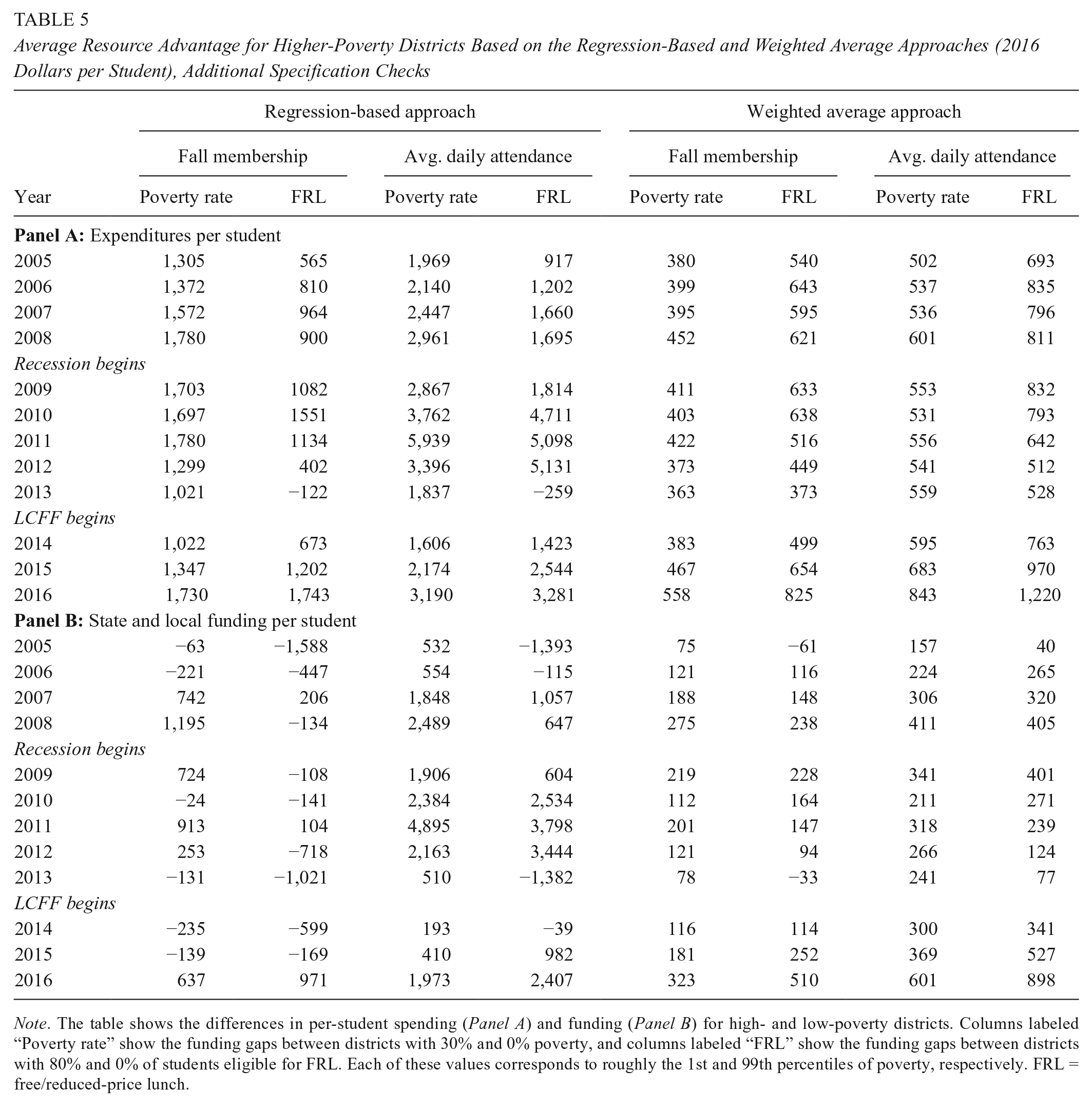
Note. The table shows the differences in per-student spending (Panel A) and funding (Panel B) for high- and low-poverty districts. Columns labeled “Poverty rate” show the funding gaps between districts with 30% and 0% poverty, and columns labeled “FRL” show the funding gaps between districts with 80% and 0% of students eligible for FRL. Each of these values corresponds to roughly the 1st and 99th percentiles of poverty, respectively. FRL = free/reduced-price lunch.

Figure 1.

Average expenditure rates for high- and low-poverty districts and spending advantage for higher-poverty districts. (A) Regression-based approach. (B) Weighted average approach.

Figure 2.

Average funding rates and funding advantage for higher-poverty districts. (A) Regression-based approach. (B) Weighted average approach.

Figure 3.

School finance equity in California, ranking relative to other states, 2004–2005 to 2015–2016. (A) Regression based, expenditures per student. (B) Weighted average, expenditures per student. (C) Regression based, state and local revenues per student. (D) Weighted average, state and local revenues per student.

Figure 4.

Comparing the regression-based approach and the weighted average approach based on state rankings, 2015–2016. (A). Expenditures per student. (B). State and local revenues per student.

Figure 5.

Funding and poverty rates for two states in which the weighted average and regression approaches to measuring state school finance diverge, 2015–2016.

Absolute Changes in School Finance Equity in California

Table 2 shows estimates of resource advantages for high-poverty districts. The first two columns show spending advantages for the regression-based approach and changes in the spending advantage over the prior year (labeled δ). The next two columns display comparable results for the weighted average approach. The final four columns show the same set of results, but for state and local funding rather than expenditures. We note the beginning of the Great Recession following the 2007–2008 school year, because 2008–2009 is the first school year in which the Recession began affecting school district finances (Baker, 2014a; Knight, 2017).

The left side of Table 2 shows the results for expenditures per student. School finance equity for low-income students in California decreased after the onset of the Great Recession, especially during the 2 years prior to the beginning of LCFF. The results for the regression-based approach, in column 1, show that in 2010–2011, the highest-poverty districts spent $1,780 more than the lowest-poverty districts but spending advantage decreased by $480 and then by $279, down to $1,021 per student, in the subsequent 2 years. Spending advantage increased to $1,730 by 2015–2016, 3 years after the implementation of LCFF began. The next two columns show the results for the weighted average approach. As with the regression-based approach, the results for the weighted average approach show that equity decreased in the 2 years leading up to LCFF and then increased in the following 3 years. Although the changes over time in spending advantage are consistent between the two measures, the weighted average approach identifies much smaller spending advantages. This finding make sense given that the regression approach estimates funding differences between the lowest- and highest-poverty districts (0% and 30% poverty rates, respectively), whereas the weighted average approach estimates spending differences between the typical low-income student and typical non-low-income student. In the 2015–2016 school year, for example, the average non-low-income student and average low-income student attended school in a district where the poverty rate was 17.8% and 23.2%, respectively.

The results in the left portion of Table 2 are synthesized in Figure 1, which shows estimates of expenditure per student in high- and low-poverty districts for the regression-based approach (Panel A) and the weighted average approach (Panel B). The lines indicate expenditure rates for each type of district, and the gray bars represent the spending advantage. The regression-based approach shows that the level of equity increased following the implementation of LCFF but has not returned to pre-Recession levels, whereas the weighted average approach suggests that the state has a more equitable system now than at any other time in the past two decades.

Figure 2 and the right side of Table 2 display the same results for state and local funding. The results for the regression-based approach (Panel A of Figure 2) suggest that, unlike expenditures, funding is distributed regressively for much of the early 2000s. This funding gap finally disappears in the years leading up to the Great Recession, but the system becomes less equitable during the Recession, including during the 2 years leading up to LCFF. Results based on the weighted average approach (Panel B of Figure 2) tell a similar story. For both expenditure and funding, LCFF is associated with greater finance equity, but the weighted average approach provides a more favorable estimate of the extent to which equity increases after LCFF. Like most other states, the California school finance system is generally more equitable in terms of expenditures than with state and local funding.¹⁴

Relative Changes in School Finance Equity in California

How do absolute changes in school finance equity in California compare with other states, and how do relative changes vary across equity measures? Figure 3 shows California’s ranking in school finance equity relative to other states. Consistent with the absolute changes shown in Figures 1 and 2, school finance equity in California increases relative to other states leading up to the Great Recession, decreases following the beginning of the Recession, and then increases after LCFF is implemented. This trend is consistent across equity measures and for both spending and funding. As with absolute measures of equity, the weighted average approach shows greater increases in equity following the implementation of LCFF.¹⁵ For both spending and funding, the regression-based approach places California in a higher rank than the weighted average approach for much of the 2000s but in a lower rank in the most recent years. In other words, across school years, one approach to measuring school finance equity does not consistently place the state in a higher rank than the other. Differences in the two equity measures, then, may be related to characteristics that change within a state over time. Below we describe some state characteristics associated with differences in the two equity measures.

Exploring Differences in Regression and Weighted Average Equity Measures

To gain a deeper understanding of the alignment between the regression-based and weighted average approaches to assessing school finance equity, we first show how the two measures align for each state in 2015–2016. For states located along the dashed lines in Figure 4, the two measures are relatively aligned. For those above the dashed line, the regression approach places states at a higher ranking in terms of school finance equity than the weighted average approach. As is clear, while the weighted average approach places California in a higher ranking than the regression approach, the two measures are fairly well aligned for California compared with some other states such as Florida, New York, Maryland, and Pennsylvania. The two measures have somewhat greater alignment overall for state and local revenues than for expenditures per student (more of the states in Panel B are near the dashed line than those in Panel A).¹⁶

Summary Statistics

Next, we summarize the state characteristics associated with differences between the regression-based and weighted average approaches. We construct a state-by-year data set for 49 states from 2004–2005 to 2015–2016, excluding Hawaii and Washington, D.C. (since both represent one school district). To equalize the overall variation in equity estimates between the two measures, we standardize each measure to a mean of 0 and standard deviation of 1 across states and school years.¹⁷ We take two approaches to comparing the regression and weighted average approaches. The absolute value of the difference shows the overall convergence of the two measures. We also examine the difference between the regression and weighted average approaches, where positive values suggest that the regression approach estimates a greater degree of equity than the weighted average approach. Panel A of Table 3 shows summary statistics of state characteristics, based on quintiles of the absolute value of the difference between the regression and weighted average approaches, measured using expenditures per student in 2015–2016. States in the first quintile—those for which the two measures most closely align—have a greater number of school districts and higher levels of income-based segregation. Conversely, states in which the two measures are poorly aligned have larger (but fewer) school districts, less segregation, a lower range of overall poverty across districts, and are generally more equitable.

Panel B provides insight into why one measure may be greater or less than the other. States in the first quintile in Panel B—those for which the weighted average approach estimates greater equity than the regression approach—are more segregated, but there is no clear pattern for the other variables. In contrast, states in which the weighted average approach estimates less equity than the regression approach (the fifth quintile) are less segregated, but they also have fewer (and larger) districts and a narrower range of average poverty across districts. Parallel results for state and local revenues are qualitatively similar and are reported in Appendix Table A1.

Regression Results

Finally, Table 4 gives the regression coefficients predicting the difference in equity measures for the regression and weighted average approaches, using the state-by-year panel described earlier (n = 588).¹⁸ The coefficients in the odd-numbered columns are based on bivariate regressions. For the even-numbered columns, we add all state covariates simultaneously. All variables are standardized to allow for comparisons across coefficients. Column 1 shows that a larger number of districts in a state and greater segregation are associated with closer alignment between the two measures. However, only student segregation remains significant when all the variables are included in one model (column 2). The larger magnitude and statistical significance of number of districts in the bivariate regression likely result from the greater segregation in states that tend to have larger numbers of districts. Column 4 shows that the regression approach estimates greater equity than the weighted average approach in states that have higher expenditures per student and less segregation. As with equity measures based on spending, those based on state and local revenues are more closely aligned in states with more across-district segregation (column 6). The measures are also more closely aligned in states with fewer districts, lower average spending, and a narrower range of poverty across districts. However, as shown in column 8, although these variables explain the absolute differences between the two equity measures, none are statistically significantly related to the overall difference. In summary, the two measures are more closely aligned in states with more income-based segregation across districts, but the regression approach generally estimates less equity than the weighted average approach for more segregated states.

Additional Variables and Extensions

We estimate two sets of additional models to gauge the sensitivity of our results to alternate specifications. First, we exchange the census-based poverty rate with the percentage of students eligible for FRL. As noted in recent research, the two measures are moderately correlated (.79 in California across all years; see Chingos, 2016; Domina et al., 2018; Harwell & LeBeau, 2010). To estimate resource gaps, we predict spending and funding levels for districts with 0% and 80% FRL students, corresponding to approximately the same percentiles of census poverty rates (roughly the 1st and 90th percentiles, respectively). Second, we exchange the fall membership variable with ADA, which measures the average number of students attending school each day. California uses this measure to allocate funding, and several recent analyses of LCFF also use ADA rather than fall membership.¹⁹

The results for these alternate specifications are given in Table 5. The first two columns show estimated spending and funding advantages for two models that both use fall membership but differ in the measure of student poverty (column 1 is repeated from Table 2 for comparison purposes). Given that U.S. Census poverty rates are based on surveys of households and FRL, in most cases, is based on students voluntarily returning application forms, the Census poverty rates are likely a more accurate depiction of the true poverty rate. This measure is still imperfect in part because not all students living in a district’s attendance zone attend schools in that district.

We find that in all years, the funding advantage for high-poverty districts is smaller, or the funding disadvantage is greater, when FRL is used in place of the U.S. Census poverty rate. In other words, using FRL as an indicator of poverty makes the school finance system appear less equitable. This may result from ceiling effects in the percentage of FRL students. The distribution of the percentage of FRL students across districts is approximately normal, with a mean of about 50%. In contrast, Census poverty rates have a mean of about 20%, with a long tail that stretches up to 100%. Thus, among districts with greater than 90% of FRL students, Census poverty rates generally range from 30% up to 70% or more. Greater funding allocated to the very highest-poverty districts may not be observed in models that use the percentage of FRL students. To test this pattern, we create a variable that measures the difference between a district’s standardized poverty rate and standardized percent FRL. We regress this variable on state and local funding per student and district controls and find that a higher rate of poverty relative to the percentage of FRL students is positively associated with funding, implying that districts receive greater funding with higher Census poverty rates at any given level of the percentage of FRL students. Using the percentage of FRL students to assess income-based across-district school finance equity may therefore mask some of the progressivity associated with funding allocated to the very highest-poverty districts.

Federal guidelines allow states to use “community eligibility” policies that allow schools above a certain threshold of percentage of FRL students to provide FRL to all students, effectively raising the proportion of FRL students in some schools to 100%. To test for the potential presence of community eligibility, we create histograms of the percentage of FRL students across schools in a state, using school-level data from NCES. Appendix Figure A3 shows that in many states, including California, community eligibility policies do not appear to change the shape of the distribution of the percentage of FRL students across schools. In other states, such as Mississippi and New Mexico, there is a large spike in the number of schools reporting 100% FRL students, compared with the number reporting 99%.

The next two columns in Table 5 show the same results, based on ADA. Not surprisingly, using ADA as a measure of the number of students a district serves tends to overstate the degree of equity. Because higher-poverty districts tend to have lower attendance rates, using ADA as the denominator in measures of per-student spending and funding will overstate resource levels relative to districts with higher rates of attendance. This pattern of results holds for estimates based on the weighted average approach. Importantly, several states, including California, fund districts based on ADA (Knight & Olofson, 2018). Some scholars argue that ADA is actually a better indicator of costs than enrollment because schools do not incur costs for students who are not in attendance. Baker (2014b) explains some limitations in this line of argument. Even if most students never have perfect attendance, all students attend school for some portion of the school year, so schools must choose the number of desks and make staffing decisions based on district enrollment rather than district attendance. In short, while previous analyses of state school finance use ADA, evidence suggests that fall enrollment is likely a stronger indicator of district costs. Using ADA artificially inflates estimates of school finance equity.

Discussion

Relative funding and spending for low-income students increased during the 3 years following implementation of the LCFF school finance reform.²⁰ In general, the weighted average approach estimates a higher degree of income-based equity for California than the regression-based approach, and a larger increase in equity following the implementation of LCFF. However, the two measures are more closely aligned in California than they are in most other states, in part because California has a large number of relatively segregated districts. Below, we describe the limitations of the study and recommendations for future research and policy.

Caveats and Limitations

Our analyses provide insights into the extent to which school finance equity in California improved following the implementation of LCFF and, more broadly, how alternate data sources and methodological approaches can produce different estimates of resource equity. A few caveats are warranted. First, district-level studies of resource allocation omit analysis of within-district resource allocation. States with larger and more segregated districts, such as California, Florida, and Maryland, are more likely to have within-district resource disparities (Knight, 2019; Orfield & Frankenberg, 2014; Sosina & Weathers, 2019). Hill and Ugo (2015) identify a number of schools in California where the percentage of low-income or English learner students exceeds 90% yet the district rate is below 25%. To determine whether LCFF, or similar reforms, targets resources to high-need students, further research should analyze within-district resource allocation (e.g., Lafortune, 2019).

Second, our study does not explore the types of educational practices in which districts are investing. Although such analyses are beyond the scope of this article, the methods used in this study could be adapted to specific types of spending categories, such as instruction, student support, and administration.

Third, we emphasize that our intent is not to estimate the causal impact of LCFF on school finance trends. Instead, our purpose is to describe how funding rates changed for different types of districts (low and high poverty) as the policy was implemented. Johnson and Turner (2018), in contrast, use a synthetic instrumental variables approach to answer two questions: (1) Did LCFF increase spending for the districts that were intended to receive additional resources? (2) What was the causal impact on student outcomes of each additional dollar of spending? We argue that both types of analyses offer important lessons for policy. Policymakers may benefit from knowing, in a general sense, how funding equity changed after the policy was implemented, overall and relative to other states.²¹ But policymakers also want to know if, net of other factors, LCFF accomplished one of its central goals of increasing state aid for historically underserved students and, if so, whether that increase in funding led to improved student outcomes.²²

Implications for Research and Policy

We highlight three key implications of our work. First, the two most prominent methods for measuring school finance equity lead to different conclusions in some states. Which measure is correct? The answer depends on both theoretical and practical considerations. For states with more socioeconomically (or racially) integrated school districts (e.g., Arkansas, North Carolina, and Tennessee), the regression approach estimates higher degrees of equity as long as there is at least a moderate positive relationship between district poverty (or the percentage of students of color) and funding. That is, the regression approach is more sensitive to funding differences in more integrated states and less sensitive to funding differences in more segregated states. Under the regression approach, states with more segregated districts require strongly progressive funding patterns to have high levels of finance equity. For the weighted average approach, a more integrated state would need strongly progressive funding to rank highly in school finance equity. The weighted average approach is more sensitive to funding differences in more segregated states (and less sensitive in more integrated states) and thus disproportionately “rewards” segregation. The regression approach therefore better aligns with the theoretical position that low-income students should receive especially more resources when such students attend school in districts that are segregated from wealthier districts. From a practical standpoint, because the regression approach forces a linear relationship, the measure will not perform well in states with a small number of districts (e.g., the six states with fewer than 50 districts).²³

This trend can be seen by comparing equity measures in two illustrative states. Pennsylvania, a state with high income-based segregation, ranks 24th in school funding equity based on the regression approach, but it ranks 13th based on the weighted average approach. In contrast, North Carolina has less student segregation and ranks 11th nationally in school funding equity based on the regression approach but 23rd based on the weighted average approach. The regression approach suggests that the North Carolina system is more equitable than Pennsylvania’s, whereas the weighted average approach shows Pennsylvania’s system as more equitable. Both states have more than 100 districts, so the linear relationship estimated in the regression approach is unlikely to provide an imprecise or skewed estimate of equity. The left panel of Figure 5 shows that Pennsylvania has a flat relationship between funding and poverty rate, and as a result, the state ranks poorly in the regression-based approach. However, the largest district in the state, Philadelphia (the largest circle), has slightly above-average funding and a far greater poverty rate than the state average. Allentown, Reading, and Pittsburgh are also high-poverty districts with above-average funding rates. Although the regression is weighted by enrollment, the slightly greater funding in a small number of large districts is not enough to increase the slope of the regression line. However, those larger, higher-poverty districts cause the weighted average approach to identify greater equity, placing the state 13th nationally. In general, those states farthest from the dashed lines in Figure 4 tend to have the highest or lowest levels of segregation.

North Carolina provides the opposite story. Funding in North Carolina is more progressive based on the regression approach (ranked 11th in 2015–2016); however, because districts are more socioeconomically integrated, the typical low-income student attends a district with approximately the same level of poverty as the typical non-low-income student. Therefore, the weighted average approach identifies little funding equity and ranks the state 23rd nationally. Neither measure is incorrect; they just assume a slightly different perspective on equity: The weighted average approach emphasizes the experience of the typical low-income student, and the regression approach focuses on the highest- and lowest-poverty districts in the state. Under this framework, the level of student segregation is an important predictor of how well the two measures align. In a relatively equitable school finance system, greater integration tends to amplify the level of equity based on the regression approach but reduces estimates of finance equity in the weighted average approach.²⁴

This finding has clear implications for future research on school finance equity, but there are also implications for policy. State efforts to reduce disparities in school resources across districts sometimes focus on reducing across-district student segregation rather than increasing funding in high-poverty districts or districts serving higher percentages of students of color (Finnigan & Holme, 2015). If the state initially has an inequitable system, then desegregation efforts may cause the state’s finance system to appear even less equitable on national reports that use the regression-based approach since the slope of the regression line would become steeper and more negative as the highest- and lowest-poverty districts move toward the mean poverty rate. States engaged in school finance equity reforms may need to be mindful of how these efforts will be assessed and reported in the media. Knowing how particular equity reforms such as desegregation or targeted funding increases will be assessed in national reports will help states build and sustain support for their equity-based policies.

Second, as noted in prior literature, FRL is an imperfect measure of income. Our study adds to this conversation by clarifying some additional implications of this fact. We highlight the variation in Census poverty rates among highest-FRL districts. Since high-FRL districts that also have extremely high poverty rates (e.g., above 50%) receive more funding on average nationally than otherwise similar high-FRL districts with more moderate poverty rates (e.g., between 25% and 50%), the use of FRL may understate income-based measures of school finance equity. Conversely, some state school finance formulas might treat high-FRL districts equally, even though some high-FRL districts may have greater poverty rates than other high-FRL districts. States may consider using U.S. Census poverty rates or other indicators of household income in their school finance formulas because Census poverty rates are less likely to suffer from ceiling effects. These issues may be complicated by FRL community eligibility provisions, although we show that use of community eligibility is not prominent in all states. Notably, district-level Census poverty rates can be easily linked to other databases through publicly available data, including those specifically designed for school finance analyses (e.g., Education Law Center, 2018; Urban Institute, 2018).

Last, state education agencies should consider publishing links or data crosswalks between state and federal data systems. Such a process would increase transparency around these two data sources and allow state and federal education officials to feel more comfortable reading and working with data outside their own agencies. To demonstrate how this might work, we include in our Appendix, STATA code that uses raw data downloaded from CDE and creates funding variables that align with U.S. Census data. Greater proliferation and transparency of these types of crosswalks will encourage researchers to review one another’s data-cleaning procedures and help ensure that data sources are correctly aligned.

Conclusion

For many years, scholars have debated the merits of school finance reforms that increased funding for high-poverty districts (Greenwald, Hedges, & Laine, 1996; Hanushek, 1986, 1997). Some researchers have argued that there is no clear and consistent relationship between substantial long-term increases in funding and student outcomes (e.g., Hanushek, 1997). However, based on studies using more robust data and methods than were previously available, scholars have now largely reached a consensus that school finance reforms are a powerful mechanism for increasing educational opportunity. As a result, the significance of research on school finance in general and school finance equity in particular has increased precipitously. Accurate measurement of school finance equity, with greater understanding of how particular theoretical perspectives, analytic approaches, and data sources influence results, will better inform policy efforts to improve state school finance systems.

Footnotes

Appendix A

Table A2

Correlation Matrix for Two State School Finance Equity Measures, the Difference Between Those Two Measures, and State-Level Characteristics, 2004–2005 to 2015–2016

	Regression Approach	Weighted Average Approach	Difference Between Standardized Values of Regression and Weighted Average Approaches	Absolute Value of Difference Between Standardized Values of Regression and Weighted Average approaches
Panel A: Expenditures per student
Equity measures
Regression approach	1
Weighted average approach	0.757	1
Difference between standardized values of regression and weighted average approaches	0.349	−0.349	1
Absolute value of difference between standardized values of regression and weighted average approaches	0.182	0.309	−0.181	1
State characteristics
Number of districts	−0.117	−0.009	−0.155	−0.213
Average district size	−0.183	−0.232	0.071	0.190
Average expenditure per student	0.203	0.150	0.077	0.097
Average poverty rate	−0.203	−0.239	0.053	−0.113
Poverty range (across districts)	0.040	0.161	−0.173	−0.210
Dissimilarity index	−0.019	0.245	−0.378	−0.247
Panel B: State and local revenues per student
Equity measures
Regression approach	1
Weighted average approach	0.862	1
Difference between standardized values of regression and weighted average approaches	0.263	−0.263	1
Absolute value of difference between standardized values of regression and weighted average approaches	−0.027	0.108	−0.256	1
State characteristics
Number of districts	−0.039	−0.080	0.078	−0.042
Average district size	−0.039	−0.034	−0.009	0.186
Average expenditure per student	0.179	0.213	−0.064	0.323
Average poverty rate	−0.012	−0.130	0.225	−0.032
Poverty range (across districts)	−0.007	−0.084	0.147	−0.266
Dissimilarity index	0.102	0.099	0.004	−0.135

Appendix B

Funding

The author(s) disclosed receipt of the following financial support for the research, authorship, and/or publication of this article: This material is based upon work supported by the National Science Foundation under Grant No. 1661097 and Grant No. 1945937. Any opinions, findings, and conclusions or recommendations expressed in this material are those of the authors and do not necessarily reflect the views of the National Science Foundation.

ORCID iD

David S. Knight

Notes

Authors

DAVID S. KNIGHT is an assistant professor of education finance and policy at the University of Washington College of Education. His research focuses on school finance, educator labor markets, and cost-effectiveness analysis.

JESÚS MENDOZA is an economic analyst for the city of El Paso. He completed his master’s degree in economics from the University of Texas at El Paso. His research examines public economics and economics of education.

References

Affeldt

J. T.

(2015). New accountability in California through local control funding reforms: The promise and the gaps. Education Policy Analysis Archives, 23(23). Retrieved from https://epaa.asu.edu/ojs/article/view/2023/1554

Angrist

J. D.

Pischke

J. S.

(2008). Mostly harmless econometrics: An empiricist’s companion. Princeton, NJ: Princeton University Press.

Atchison

Baker

Boyle

Levin

Manship

(2017). Exploring the quality of school-level expenditure data: Practices and lessons learned in nine sites. Washington, DC: Office of Planning, Evaluation and Policy Development, U.S. Department of Education.

Baker

B. D.

(2014a). Evaluating the Recession’s impact on state school finance systems. Education Policy Analysis Archives, 22(91). Retrieved from https://epaa.asu.edu/ojs/article/view/1721/1357

Baker

B. D.

(2014b). Not making the grade: How financial penalties for school absences hurt districts serving low-income, chronically ill kids. Oakland, CA: Change Lab Solutions.

Baker

B. D.

(2016). School finance and the distribution of equal educational opportunity in the post recession US. Journal of Social Issues, 72, 629–655.

Baker

B. D.

Corcoran

S. P.

(2012). The stealth inequities of school funding: How state and local school finance systems perpetuate inequitable student spending. Washington, DC: Center for American Progress.

Baker

B. D.

Farrie

Sciarra

D. G.

(2018). Is school funding fair? A national report card (7th ed.). Newark, NJ: Education Law Center.

Baker

B. D.

Farrie

Johnson

Luhm

Sciarra

D. G.

(2017). Is school funding fair? A national report card (6th ed.). Newark, NJ: Education Law Center.

10.

Baker

B. D.

Farrie

Luhm

Sciarra

D. G.

(2016). Is school funding fair? A national report card (5th ed.). Newark, NJ: Education Law Center.

11.

Baker

B. D.

Green

P. C.

(2015). Conceptions of equity and adequacy in school finance. In Ladd

H. F.

Goertz

M. E.

(Eds.), Handbook of research in education finance and policy (2nd ed., pp. 231–242). New York, NY: Routledge.

12.

Baker

B. D.

Green

P. C.

III Ramsey

M. J.

(2018). Financing education for children with special needs. In Handbook of leadership and administration for special education (pp. 130–147). New York, NY: Routledge.

13.

Baker

B. D.

Sciarra

D. G.

Farrie

(2015). Is school funding fair? A national report card (4th ed.). Newark, NJ: Education Law Center.

14.

Berne

Stiefel

(1979). Taxpayer equity in school finance reform: The school finance and the public finance perspectives. Journal of Education Finance, 5, 36–54.

15.

Berne

Stiefel

(1984). The measurement of equity in school finance. Baltimore, MD: Johns Hopkins Press.

16.

Berne

Stiefel

(1994). Measuring equity at the school level: The finance perspective. Educational Evaluation and Policy Analysis, 16, 405–421.

17.

Brunner

E. J.

Vincent

J. M.

(2018). Financing school facilities in California: A ten-year perspective (Getting Down to Facts II Technical Report). Retrieved from https://www.gettingdowntofacts.com/sites/default/files/2018-09/GDTFII_Report_Brunner-Vincent.pdf

18.

Bruno

(2018). District dollars 2: California school district finances, 2004–05 through 2016–17 (Getting Down to Facts II Technical Report). Retrieved from http://www.gettingdowntofacts.com/sites/default/files/2018-09/GDTFII_Report_Bruno.pdf

19.

California Department of Education. (2016). California school accounting manual. Sacramento, CA: Author.

20.

Candelaria

C. A.

Shores

K. A.

(2019). Court-ordered finance reforms in the adequacy era: Heterogeneous causal effects and sensitivity. Education Finance and Policy, 14, 31–60. doi:10.1162/edfp_a_00236

21.

Card

Payne

A. A.

(2002). School finance reform, the distribution of school spending, and the distribution of student test scores. Journal of Public Economics, 83, 49–82.

22.

Chingos

(2016). No more free lunch for education policymakers and researchers (Evidence Speaks Reports, Vol. 1, #20). Washington, DC: Brookings Institute.

23.

Chingos

M. M.

Blagg

(2017). Do poor kids get their fair share of school funding? Washington, DC: Urban Institute.

24.

Conaway

(2019). Maximizing research use in the world we actually live in: Relationships, organizations, and interpretation (CALDER Policy Brief No. 14-0319-1). Washington, DC: National Center for Analysis of Longitudinal Data in Education Research.

25.

Cornman

S. Q.

(2016). Documentation for the NCES Common Core of Data National Public Education Financial Survey (NPEFS), School Year 2013–14 (Fiscal Year 2014) (NCES 2016-302). Washington, DC: U.S. Department of Education, National Center for Education Statistics, Institute of Education Sciences.

26.

Costrell

R. M.

(2005). Equity v. equity: Why Education Week and the Education Trust don’t agree. Education Next, 5(3), 77-81.

27.

Darity

Jr. Castellino

Tyson

Cobb

McMillen

(2001). Increasing opportunity to learn via access to rigorous courses and programs: One strategy for closing the achievement gap for at-risk and ethnic minority students. Durham: North Carolina Department of Public Instruction.

28.

Domina

Pharris-Ciurej

Penner

A. M.

Penner

E. K.

Brummet

Porter

S. R.

Sanabria

(2018). Is free and reduced-price lunch a valid measure of educational disadvantage? Educational Researcher, 47, 539–555. doi:10.3102/0013189X18797609

29.

Dowd

A. C.

Bensimon

E. M.

(2015). Engaging the “race question”: Accountability and equity in US higher education. New York, NY: Teachers College Press.

30.

Duncombe

Yinger

(2007). Does school district consolidation cut costs? Education Finance and Policy, 2, 341–375.

31.

Education Law Center. (2018). School funding data. Retrieved from http://www.edlawcenter.org/research/school-funding-data.html

32.

Evans

W. N.

Schwab

R. M.

Wagner

K. L.

(2019). The Great Recession and public education. Education Finance and Policy, 14, 298–326. doi:10.1162/edfp_a_00245

33.

Finnigan

K. S.

Holme

J. J.

(2015). Regional educational equity policies: Learning from inter-district integration programs (Research Brief No. 9). Washington, DC: National Coalition on School Diversity.

34.

Fuller

Tobben

(2014). Local Control Funding Formula in California: How to monitor progress and learn from a grand experiment. Berkeley, CA: Chief Justice Earl Warren Institute on Law and Social Policy and Partners for Each and Every Child. Retrieved from https://files.eric.ed.gov/fulltext/ED561883.pdf

35.

Greenwald

Hedges

L. V.

Laine

R. D.

(1996). The effect of school resources on student achievement. Review of Educational Research, 66, 361–396.

36.

Grubb

W. N.

(2009). The money myth: School resources, outcomes and equity. New York, NY: Russell Sage Foundation.

37.

Hanushek

E. A.

(1986). The economics of schooling: Production and efficiency in public schools. Journal of Economic Literature, 24, 1141–1177.

38.

Hanushek

E. A.

(1997). Assessing the effects of school resources on student performance: An update. Educational Evaluation and Policy Analysis, 19, 141–164.

39.

Harwell

LeBeau

(2010). Student eligibility for a free lunch as an SES measure in education research. Educational Researcher, 39, 120–131.

40.

Hill

Ugo

(2015). Implementing California’s school funding formula: Will high-need students benefit? Sacramento: Public Policy Institute of California.

41.

Humphrey

D. C.

Koppich

J. E.

Esch

Marsh

J. A.

Hall

Campbell

. . . Imazeki

(2014). Toward a grand vision: Early implementation of California’s Local Control Funding Formula. Menlo Park, CA: J. Koppich & Associates/SRI International.

42.

Jackson

C. K.

Johnson

R. C.

Persico

(2015). The effects of school spending on educational and economic outcomes: Evidence from school finance reforms. Quarterly Journal of Economics, 131, 157–218.

43.

Johnson

R. C.

Tanner

(2018). Money and freedom: The impact of California’s school finance reform on academic achievement and the composition of district spending (Getting Down to Facts II Technical Report). Retrieved from http://www.gettingdowntofacts.com/sites/default/files/2018-09/GDTFII_Report_Johnson.pdf

44.

Knight

D. S.

(2017). Are high-poverty school districts disproportionately impacted by state funding cuts? School finance equity following the Great Recession. Journal of Education Finance, 43, 169–194.

45.

Knight

D. S.

(2019). Are school districts allocating resources equitably? The Every Student Succeeds Act, teacher experience gaps, and equitable resource allocation. Educational Policy, 33, 615–649. doi:10.1177/0895904817719523.

46.

Knight

D. S.

DeMatthews

D. E.

(2017). Assessing the educational opportunity of emergent bilingual students: Why are some state school finance systems more equitable than others? (CERPS Working Paper 2017-1). University of Texas at El Paso, El Paso.

47.

Knight

D. S.

Mendoza

J. E.

(2019). Compounded inequities: Tracking school finance equity for districts serving low-income emergent bilingual students. In DeMatthews

D. E.

Izquierdo

(Eds), Dual language education: Teaching and leading in two languages (pp. 35–55). New York, NY: Springer.

48.

Knight

D. S.

Olofson

(2018, July). Funding school districts based on student attendance: How use of average daily attendance harms school finance equity in Texas (Policy Brief #5). El Paso, TX: Center for Education Research and Policy Studies.

49.

Knight

D. S.

Strunk

K. O.

(2016). Who bears the costs of district funding cuts? Reducing inequality in the distribution of teacher layoffs. Educational Researcher, 45, 395–406.

50.

Knight

D. S.

Toenjes

(2019). Do charter schools receive their fair share of funding? School finance equity for charter and traditional public schools. Educational Policy Analysis Archives.

51.

Koppich

J. E.

Humphrey

D. C.

Marsh

J. A.

(2015). Two years of California’s Local Control Funding Formula: Time to reaffirm the grand vision. Policy Analysis for California Education, PACE.

52.

Ladson-Billings

Tate

W. F.

(2016). Toward a critical race theory of education. In Dixson

A. D.

Rousseau Anderson

C. K.

Donnor

J. K.

(Eds.), Critical race theory in education (pp. 10–31). New York, NY: Routledge.

53.

Lafortune

(2019). School resources and the Local Control Funding Formula: Is increased spending reaching high-need students? Sacramento, CA: Public Policy Institute of California.

54.

Lafortune

Rothstein

Schanzenbach

D. W.

(2018). School finance reform and the distribution of student achievement. American Economic Journal: Applied Economics, 10(2), 1–26. doi:10.1257/app.20160567

55.

Leachman

Figuera

. (2019). K-12 school funding up in most 2018 teacher-protest states, but still well below decade ago. Washington, DC: Center of Budget and Policy Priorities.

56.

Levin

(2018). Privatizing education: Can the school marketplace deliver freedom of choice, efficiency, equity, and social cohesion? New York, NY: Routledge.

57.

Levin

Brodziak de los Reyes

Atchison

Manship

Arellanes

(2018). What does it cost to educate California’s students? A professional judgment approach (Getting Down to Facts II Technical Report). Retrieved from https://www.gettingdowntofacts.com/sites/default/files/2018-09/GDTFII_Report_Levin.pdf

58.

Loeb

Grissom

J. A.

Strunk

K. O.

(2007). District dollars: Painting a picture of revenues and expenditures in California’s school districts (Getting Down to Facts Project). Palo Alto, CA: Stanford University.

59.

Mudrazija

Blagg

(2019). School district funding in Texas: Computing the effects of changes to the Foundation School Program funding formula. Washington, DC: Urban Institute.

60.

Oakes

(2005). Keeping track: How schools structure inequality. New Haven, CT: Yale University Press.

61.

Odden

Picus

(2014). School finance: A policy perspective (5th ed.). New York, NY: McGraw-Hill.

62.

Orfield

Frankenberg

(2014). Increasingly segregated and unequal schools as courts reverse policy. Educational Administration Quarterly, 50, 718–734.

63.

Picus

L. O.

Goertz

Odden

A. R.

(2015). Intergovernmental aid formulas and case studies. In Ladd

H. F.

Goetz

M. E.

(Eds.), Handbook of research in education finance and policy (2nd ed., pp. 279–296). New York, NY: Routledge

64.

Picus

L. O.

Odden

A. R.

Griffith

Hoyer

Knight

D. S.

Odden

(2016). Using the evidence-based method to identify adequate spending levels for Vermont schools (A report prepared for the Vermont State Legislature). North Hollywood, CA: Picus, Odden, & Associates.

65.

Rawls

(1971). A theory of justice. Cambridge, MA: Harvard University Press

66.

Rivera

M. D.

Lopez

S. R.

(2019). Some pennies are more equal than others: Inequitable school facilities investment in San Antonio, Texas. Education Policy Analysis Archives, 27(16). Retrieved from https://epaa.asu.edu/ojs/article/view/4191

67.

Rodriguez

G. M.

(2004). Vertical equity in school finance and the potential for increasing school responsiveness to student and staff needs. Peabody Journal of Education, 79(3), 7–30.

68.

Rose

Weston

(2013). California school district revenue and student poverty: Moving toward a weighted pupil funding formula. Sacramento: Public Policy Institute of California. Retrieved from https://www.ppic.org/content/pubs/report/R_213HRR.pdf

69.

Shores

Ejdemyr

(2017). Pulling back the curtain: Intra-district school spending inequality and its correlates. Unpublished manuscript. Retrieved from http://dx.doi.org/10.2139/ssrn.3009775

70.

Sosina

V. E.

Weathers

E. S.

(2019). Pathways to inequality: Between-district segregation and racial disparities in school district expenditures. AERA Open, 5(3). doi:10.1177/2332858419872445.

71.

Spring

(2016). Deculturalization and the struggle for equality: A brief history of the education of dominated cultures in the United States. New York, NY: Routledge.

72.

Taylor

L. L.

(2004). “Adjusting for geographic variations in teacher compensation: Updating the Texas Cost-of-Education Index. A report prepared for the Texas Legislature Joint Committee on Public School Finance. Retrieved from: http://bush.tamu.edu/research/faculty/TXSchoolFinance/

73.

Taylor

L. L.

(2015). When equal is not equitable: Adjusting for geographic differences in education costs. The Takeaway, 6(4), 1–4.

74.

Taylor

L. L.

Fowler

W. J.

Jr. (2006). A comparable wage approach to geographic cost adjustment (Research and Development Report NCES-2006-321). Washington, DC: National Center for Education Statistics.

75.

Taylor

(2013). Updated: An overview of the Local Control Funding Formula. Sacramento, CA: Legislative Analyst’s Office.

76.

Urban Institute. (2018). Education data portal (Beta). Retrieved from https://educationdata.urban.org/documentation/

77.

Ushomirsky

Williams

(2015). Funding gaps 2015: Too many states still spend less on educating students who need the most. Washington, DC: Education Trust.

78.

Verstegen

D. A.

(1996). Concepts and measures of fiscal inequality: A new approach and effects for five states. Journal of Education Finance, 22, 145–160.

Does the Measurement Matter? Assessing Alternate Approaches to Measuring State School Finance Equity for California’s Local Control Funding Formula

Abstract

Keywords

Background on School Finance Equity and the LCFF

Theoretical Conceptions of School Finance Equity

Measurement of School Finance Equity

Simple Measures of School Finance Equity

Advanced Measures of School Finance Equity

Data Sources for Measuring School Finance Equity

School Finance Equity in California Under the LCFF

Data and Analytic Approach

Aligning State and Federal Finance Data

Measures of School Finance Equity

Findings

Main Results

Absolute Changes in School Finance Equity in California

Relative Changes in School Finance Equity in California

Exploring Differences in Regression and Weighted Average Equity Measures

Summary Statistics

Regression Results

Additional Variables and Extensions

Discussion

Caveats and Limitations

Implications for Research and Policy

Conclusion

Footnotes

Appendix A

Appendix B

Funding

ORCID iD

Notes

Authors

References