Sage Journals: Discover world-class research

Abstract

This article examines how teachers unions affect teachers’ well-being under various legal institutions. Using a district–teacher matched data set, this study identifies the union effects by three approaches. First, I contrast teacher outcomes across different state laws toward unions. Second, I compare the union–nonunion differentials within the same legal environment, using multilevel models and propensity score matching. Finally, unexpected legal changes restricting the collective bargaining of teachers in four states form a natural experiment, allowing me to use the difference-in-difference estimation to identify the causal effect of weakening unionism on teacher outcomes. I find that (a) many teachers join unions even when bargaining is rarely or never available, and meet-and-confer or union membership rate affects teachers’ lives in the absence of a bargaining contract; (b) how unions influence teacher outcomes vary greatly by different legal environment; and (c) the changes in public policy limiting teachers’ bargaining rights significantly decrease teacher compensation.

Keywords

employer–employee matched data teachers unions collective bargaining meet-and-confer multilevel model propensity score matching

Over half of union workers in the United States are in the public sector, and public school teachers comprise the single largest group of public sector unions. In 2018, governments employed approximately 3.2 million public school teachers, of whom about 65% were union members. Contrasted with private sector unions regulated by the country’s single labor law, the 1935 National Labor Relations Act,¹ the unions of public sector employees encounter different legal institutions, depending on geographic region. Some states, for instance, allow collective bargaining and strikes by public school teachers, whereas others ban teachers from engaging in these activities.

The federal labor law also plays an important role for teachers’ well-being. In 1977, the Supreme Court in Abood v. Detroit Board of Education upheld public sector agency shop clauses, which approve that nonunion employees who are represented by a union could be required to pay a fraction of union dues to help finance union activities. In 2018, the Supreme Court ruled in Janus v. American Federation of State, County and Municipal Employees (Janus hereafter) that the agency fees paid by public sector nonunion members violated First Amendment principles protecting freedom of speech and association. This dramatic legal change, immediately affecting the lives of teachers, has arguably shifted the course of U.S. public education.

In this post-Janus period, we are faced with a critical question regarding the role of teachers unions in public schools: How will teachers unions affect teacher outcomes and the educational system in this new legal environment? To answer this question, it is essential to understand what unions do and how they influence the educational system under different legal institutions outlined in pre-Janus settings.

The goal of this study is to examine the relationships among teachers unions, teacher pay, and working conditions and to identify channels through which teacher representation influences teachers’ well-being under different legal environments before Janus. Since teachers unions operate in widely varying legal systems, this article analyzes union effects within a group of states that share a similar legal environment regarding teachers’ collective bargaining rights.

This study sets out to examine the roles of unions by asking three key questions: First, “Is collective bargaining essential for unions to affect teacher outcomes?” Second, “How do union effects differ across different legal environments?” Last, “Does the public policy weakening the bargaining power of unions influence how unions affect teacher outcomes?”

Previous studies that focus on the existence of bargaining contracts do not capture the true variation of teacher unionization because many teachers still unionize where collective bargaining is rarely used and even where bargaining is illegal. The key contribution of this research to literature is the use of multiple measures of teacher unionization to reduce measurement errors. Employing an approach that has been largely ignored in literature, this study assesses the strength of teachers unions and examines their role in the absence of bargaining contracts.

I use the Schools and Staffing Survey (SASS) by the National Center for Education Statistics (NCES) to create a unique district–teacher matched data set. This data set provides detailed information on teacher unionization, teachers’ compensation, and working conditions; it also includes teachers’ characteristics, as well as various attributes of their schools and districts.

This study identifies the union effects by three approaches. First, I contrast teacher outcomes across different state laws, such as mandatory bargaining laws and agency shop, regarding public sector unions. Second, I compare the union–nonunion differentials within the same legal environment, using multilevel (hierarchical) linear models and propensity score matching (PSM). Finally, and most important, unexpected legal changes substantially restricting the collective bargaining of public school teachers in 2010–2011 in four states form a natural experiment, allowing me to use the difference-in-difference (DID) estimation to identify the causal effect of weakening unionism on teacher outcomes.

Literature

Literature finds that teachers unions play an important role in raising teachers’ well-being. Many studies focus on union membership to define teacher unionization and show that unions raise teacher pay. Reviews of earlier literature by Lipsky (1982), Freeman (1986), and Ehrenberg and Schwarz (1986) show that teachers unions are associated with higher salaries and that the union–nonunion wage differential is smaller among workers in the public sector than in the private sector. Baugh and Stone (1982) and Freeman and Valletta (1988) estimate the union–nonunion gap in teacher salaries to be 12% to 22%, using the Current Population Survey. Gyourko and Tracy (1991) estimate that the union wage effect is about 10% in the absence of the controls for individual teacher characteristics. Belman, Heywood, and Lund (1997) report similar estimates using the Current Population Survey outgoing rotation file for 1991. Using a district-level data set, Lemke (2004) estimates the union premium to be about 8% for public school teachers in rural areas of Pennsylvania. Zwerling and Thomason (1995) show that a 10% increase in states’ union membership rate raises the highest teacher salary by 2.6%.

Studies also look at legal institutions, such as state laws regarding teachers unions or collective bargaining agreements (CB) between districts and unions, to estimate the union effects on teacher pay. Hoxby (1996) estimates that unions raise teacher salaries by 5%, based on district-level panel data constructed from the Census of Governments data for 1972–1992. Using the district-level data for the 1999–2000 school year, Hirsch, Macpherson, and Winters (2011) estimate the effect of bargaining coverage on teacher pay to be as high as 20%. Utilizing the SASS data, Mykerezi and West (2011) and West (2015) find that CB significantly affects teacher pay schedules. Researchers also look at the “restrictiveness” of CB and find that contract strength is associated with union strength and also with higher district spending (Eberts & Stone, 1984; Strunk, 2011).

Several studies find that unions significantly improve working conditions and raise nonwage benefits. Freeman (1984, 1985) shows that employees who change to unionized jobs significantly gain nonwage benefits compared with those who stay in nonunion jobs or move out of union jobs. Freeman and Medoff (1984) attest that unionized employees are 25 to 30 percentage points more likely to report having a pension plan than comparable nonunion workers. Delaney (1985) finds that Illinois school districts with CB had a larger “fringe benefit index” compared with school districts without bargaining contracts. Eberts and Stone (1984) show that CB had a larger effect on nonwage benefits than on wages, using public school data in New York. Hirsch, Macpherson, and DuMond (1997) demonstrate that union workers are more likely to file workers’ compensation claims and to receive compensation benefits than similar nonunion workers, mainly because unions provide workers with information concerning their rights and legal benefits, as well as education in filing claims. Similarly, Budd (2007) notes that the “facilitation” role of unions serves to enhance workers’ awareness of and access to employee benefits. Podgursky (2003) argues that teachers unions in Chicago effectively increase fringe benefits, measured by pension contributions, for their members in public schools.

Since different states apply different laws toward public sector employees, researchers struggle to measure the true degree of teacher unionization, hampering the identification of union effects. For this reason, researchers often focus on limited geographic regions. For instance, Lovenheim (2009) measures unionism with union certification information in three Midwestern states that have compulsory CB laws. Rose and Sonstelie (2010) study union effects in California, a state where nearly all districts engage in CB. Brunner and Squires (2013) acknowledge this issue and present that the union impact on allocation of school resources differs greatly, depending on whether states mandate or ban CB.

This research improves on previous literature and makes several key contributions. First, I use a nationally representative data set that covers the full breadth of union laws and prevailing contracts within different legal environments. Second, the district–teacher matched data set allows me to control for districts’ characteristics, including their financial status, which were unavailable in many studies due to the lack of employer identifying information at the national level. Third, I use various metrics to gauge teacher unionization, such as state laws toward teachers unions, contractual status between districts and unions, union density of districts, and union membership of individual teachers, and examine unions’ role even in the legal environment that prohibits teachers’ CB. Finally, I conduct a comprehensive analysis on teachers’ well-being by examining teachers’ pay, working conditions, and nonwage benefits.

Legal Institutions for Teachers Unions

Until the recent efforts to limit the CB rights of public school teachers in some states, legal environments for teacher unionization have been stable for the past several decades. States that allowed CB of teachers three decades ago still do so in 2010, and districts that have CB contracts with teachers unions in 2010 are likely to have had such agreements in the 1970s. The legal institutions often reflect the general view toward teachers unions within regions and help shape and maintain the distinct environments in which local unions operate.

Following Moe (2011), I define the legal environment toward teachers unions using two legal frameworks: whether a state allows CB of public school teachers and whether it permits agency fees so that nonunion teachers pay their “fair share” fees for the services unions provide (which is no longer applicable after Janus). Based on these two legal criteria, I classify the 50 U.S. states into four groups.

Table 1 presents the group classification in detail. The first group, which I call the High-CB group, is composed of 23 states that have compulsory CB laws (also called “duty-to-bargain” laws) and allow unions and school districts to negotiate mandatory agency fees for nonunion members.² About half of public school teachers belong to this group. The second group, the Med-CB group, also has compulsory CB laws but prohibits agency fees. There are 11 states in this group, and they are located in the Midwest and South. The third group, the Low-CB group, allows local school districts to sign CB agreements but does not require them to bargain with unions. Nine states fit into this group. The fourth group, the No-CB group, bans public school teachers from collectively bargaining, and there are seven states in this group. All states but one, Arizona, are located in the South, and approximately a quarter of all public school teachers belong to this group. Figure 1 presents the map of this group categorization to visualize how these states are spread across the United States.

Table 1

Group Categorization

Group	Definition	State
High-CB (50%)	States that mandate CB and also allow agency fees	Alaska, California, Connecticut, Delaware, Hawaii, Illinois, Maine, Maryland, Massachusetts, Michigan, Minnesota, Montana, New Hampshire, New Jersey, New Mexico, New York, Ohio, Oregon, Pennsylvania, Rhode Island, Vermont, Washington, Wisconsin*
Mid-CB (15%)	States that mandate CB but ban agency fees	Florida, Idaho, Indiana, Iowa, Kansas, Nebraska, Nevada, North Dakota, Oklahoma, South Dakota, Tennessee*
Low-CB (11%)	States that do not mandate CB but allow CB	Alabama, Arkansas, Colorado, Kentucky, Louisiana, Missouri, Utah, West Virginia, Wyoming
No-CB (24%)	States that prohibit CB	Arizona, Georgia, Mississippi, North Carolina, South Carolina, Texas, Virginia

Source. “Teacher Monopoly, Bargaining, and Compulsory Unionism, and Deduction Revocation Table” by the National Right to Work Foundation, 2010, and also from Moe (2011, Table 2-2, pp. 54–55).

Note. The numbers in parentheses represent the fraction of public school teachers who belong to each group. Due to the recent legal changes in 2010–2011 regarding CB rights of teachers, states with * now are in the Low-CB group. CB = collective bargaining agreement.

Figure 1.

Group categorization.

Besides the broad legal environment toward teachers unions, there exist three types of contractual status between teachers unions and districts: a collective bargaining agreement (CB), a meet-and-confer agreement (MC), and no agreement at all (NA). All teachers unions and districts, except in the No-CB group, can specify teacher compensation and conditions of work environment, signing CB contracts that are legally binding. MC is an alternative path when districts and unions cannot come to resolution in signing bargaining contracts. During MC, both sides exchange information and opinions to reach a resolution on matters within the scope of representation, prior to adoption by the district of its final budget for the ensuing year, but the outcomes of MC are not legally enforceable.

Regardless of legal institution, unions can influence teacher outcomes by engaging in activities using their political power.³ These union activities include lobbying school districts to grant teachers higher wages or better nonwage benefits and helping elect school board members who are favorably inclined to unions’ demands. Thus, union membership rates in districts provide an additional source of power unions can wield to affect the work lives of teachers.

If studies use a dummy variable for the existence of CB, they disregard the union activity in states where CB is rarely or never used. This research conducts an elaborate analysis for assessing union effects by utilizing a wide array of indicators of union strength: state laws (High-CB, Med-CB, Low-CB, or No-CB group), contractual status (CB, MC, or NA), union membership of individual teachers, and union density of districts.

District–Teacher Matched Data

The primary data source of this study is the SASS, administered by the NCES. The SASS is large-scale and nationally representative data that cover about a third of U.S. public school districts. The SASS form multilevel data, which are composed of a series of questionnaires given to districts, schools, and teachers in the selected schools. In the 2011–2012 SASS, the most recent data to date, approximately 38,240 teachers are nested in 7,570 schools within 4,600 districts. Table A1 in Appendix A (online) presents the descriptive statistics for key variables.

By linking data on teachers, schools, and districts, I construct a district–teacher matched data set for three waves of the SASS for the 2003–2004, 2007–2008, and 2011–2012 school years. Then I merge those three district–teacher matched data sets to form a pooled cross-sectional district–teacher matched data set.

This data set provides various measures of teacher unionization. Union membership status of individual teachers is available from the teacher-level SASS, while contractual status between unions and districts is from the district-level SASS. I also compute union density by district, using union membership information from the teacher-level SASS.

Since workers’ employment and compensation levels depend on the economic situation of employers, it is critical to consider the financial status of local school districts in the analysis of the union effects (Eberts & Stone, 1985). The School Districts Finance Survey by the Education Finance Statistics Center of the NCES contains detailed annual fiscal data on public elementary and secondary education for every school district in the United States. By combining information from the School Districts Finance Survey with the SASS, this data set allows me to estimate the union–nonunion differentials among districts with similar financial status.

Hirsch, Macpherson, and Winters (2011) compare the earnings of public school teachers with those of other college graduates, who are not teachers, to examine the role of unions on teacher compensation. For a similar approach, I use the Comparable Wage Index (CWI) from the NCES. The CWI, developed by Taylor and Fowler (2006), assesses the regional variations in the salaries of college graduates in the noneducational sector.⁴ The CWI is available at the school district level, so it provides the mean for geographical comparisons for locality differences in cost of living and other labor market conditions that can otherwise contaminate the analysis due to unobservable factors in the local labor market. The CWI is also an appropriate measure of the opportunity cost of teaching over a nonteaching career in the school district.

Table 2 provides summary statistics of key variables from the pooled district–teacher matched data set, by legal group. Panel A presents the basic pattern for teachers. In the High-CB group, approximately 90% of teachers are union members. In the Low-CB group where CB is not mandated, union membership rate is as high as in the Med-CB group with duty-to-bargain laws. The surprise is that a substantial proportion (46%) of teachers still join unions in the No-CB group, where CB is illegal. The fraction of teachers with alternative certificates is highest in the No-CB group. The High-CB group has the highest proportion of teachers with a master’s degree or above. The base salary, the number of days in the normal contract year, and required working hours for base salary are most advantageous for teachers in the High-CB group.

Table 2

Summary Statistics by Legal Environment

	High-CB	Med-CB	Low-CB	No-CB
Panel A: Public school teachers
% of union member	87.9 (32.5)	63.9 (48.0)	62.4 (48.4)	45.9 (49.8)
% with alternative certificates	8.7 (28.2)	7.5 (26.3)	10.4 (29.2)	20.7 (39.5)
% with master’s degree or above	86.0 (45)	84.7 (35.9)	85.0 (35.6)	81.5 (38.7)
Base teaching salary ($)	49,533 (16,174)	38,106 (10,489)	40,831 (11,068)	41,484 (10,143)
Days in normal contract year	185.8 (21.3)	187.6 (23.4)	189.5 (23.5)	193.7 (25.2)
Required working hours	36.59 (6.11)	37.80 (5.40)	37.65 (5.73)	38.70 (4.93)
N	49,700	25,860	19,200	17,390
Panel B: Public schools
Enrollment of Grades K–12	783.7 (693.1)	740.0 (595.2)	725.6 (518.5)	847.9 (582.7)
% of students with free lunch	36.6 (26.8)	40.8 (23.7)	42.0 (22.9)	49.9 (27.1)
% of Hispanic students	11.2 (19.3)	8.8 (14.9)	6.1 (10.3)	18.5 (26.4)
% of Black students	9.78 (19.4)	8.0 (15.3)	10.5 (19.8)	27.4 (27.1)
% of Asian students	4.05 (9.30)	1.64 (2.72)	1.2 (2.1)	2.1 (3.9)
N	17,000	7,030	5,580	5,030
Panel C: School districts
% of collective bargaining districts	84.0 (36.7)	67.4 (46.8)	12.0 (32.5)	0.6 (7.9)
% of meet-and-confer districts	7.2 (25.9)	14.1 (34.9)	26.0 (43.8)	7.7 (26.7)
% of districts with no agreement	8.7 (28.2)	18.4 (38.8)	61.9 (48.5)	91.6 (27.6)
Revenue per student ($)	20,031 (16,621)	13,127 (47,906)	11,975 (13,920)	11,558 (32,622)
Benefits per teacher ($)	25,333 (84,762)	14,356 (11,502)	19,380 (14,691)	13,038 (11,789)
Benefits to total spending ratio	0.124 (0.037)	0.107 (0.028)	0.121 (0.039)	0.085 (0.030)
Log(Comparable Wage Index)	0.14 (0.13)	0.04 (0.09)	0.04 (0.10)	0.11 (0.12)
N	6,460	2,870	1,970	2,160

Source. Pooled district–teacher matched SASS (Schools and Staffing Survey) data.

Note. Standard deviations are reported in parentheses. N is rounded to the nearest ten. Teacher-level variables are weighted by teacher sample weight. School-level variables are weighted by school sample weight. District-level variables are weighted by district sample weight.

Panel B shows that public schools in the No-CB group have, on average, the highest student enrollment, the largest proportion of students eligible for free or reduced-price lunch programs, and the greatest fraction of Hispanic and Black students.

In Panel C, the majority of districts in the High-CB and Med-CB groups have CB, and MC is most popular in the Low-CB group. In the No-CB group, most districts have neither CB nor MC. Districts’ revenue per student, benefits per teacher, benefits to total spending ratio, and the CWI are highest in the High-CB group.

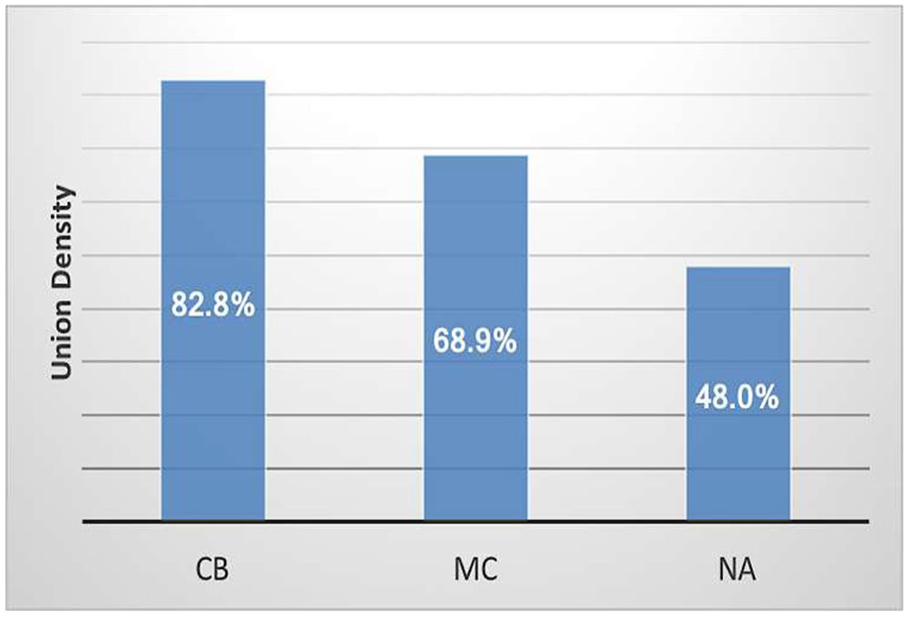
Based on the district–teacher matched data, Figures 2 through 4 highlight contradictory evidence for some widely held views about teachers unions. The first misconception is that CB is necessary for unions to attract teachers. Figure 2 shows that union density is the highest (83%) when districts have CB. However, MC districts have an approximately 70% union membership rate, and about half of teachers unionize, even in the NA districts.

Figure 2.

Union density by contractual status.

Figure 3.

Union density by union membership status.

Figure 4.

Free riders by legal environment.

The second misconception is that CB is the only avenue for public school teachers to come to an agreement with their employers. Before the enactment of labor laws permitting CB of public sector workers in the 1960s and 1970s, unions and employers commonly engaged in MC (Freeman & Ichniowski, 1988). Table 2 shows that MC is the primary form of agreement between unions and their districts in the Low-CB and No-CB groups. Figure 3 describes the contractual status by union membership status of public school teachers to confirm that MC is not an obsolete institution. Approximately 11% of union teachers and 12% of nonunion teachers are covered by MC.

The third misconception is that free riding is not a serious problem. If we define a “free rider” as a person who benefits from unions’ actions without contributing to meet their costs, there exist two types of free riders: “CB free riders” and “MC free riders.”⁵ We can estimate the extent of free riding by looking at how many nonunion teachers are in the CB and MC districts. Figure 4 presents free rider rates, measured by the fraction of nonunion teachers (nonunion density) in CB districts and MC districts. In the High-CB group, the nonunion density in CB districts is about 5%. These nonunion teachers in the High-CB group are required to pay agency fees, so they are not free riders under our definition. In the Med-CB and Low-CB groups, however, nonunion teachers are considered free riders. In the Med-CB group, 36% of teachers in the CB districts are free riders. Considering that about 70% of teachers are covered by CB in the Med-CB group, free riding will cause substantial damage to unions’ financial stability. The Low-CB group also has a high fraction of CB free riders (29%), but due to relatively low CB coverage, free riding is less likely to be a critical threat to unions’ finance than in the Med-CB group. If we take MC free riders into consideration, then the overall proportion of free riders is much greater, especially in the middle two groups.

Empirical Strategies

This study organizes the analysis around groups of states with similar legal environments toward teachers unions based on the notion that it is the legal institutions, rather than the state per se, that affects how teachers unions operate. As most state laws toward teachers unions were determined decades ago and remained generally unchanged, they provide fairly exogenous variation of teacher unionization.

I start with a general analysis using all 50 states. To examine the relationship between the legal environments and teacher outcome, I estimate the ordinary least squares (OLS) regression of the following form⁶:

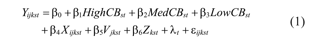
\begin{array}{l} Y_{i j k s t} = β_{0} + β_{1} H i g h C B_{s t} + β_{2} M e d C B_{s t} + β_{3} L o w C B_{s t} \\ + β_{4} X_{i j k s t} + β_{5} V_{j k s t} + β_{6} Z_{k s t} + λ_{t} + ε_{i j k s t} \end{array}

(1)

where i, j, k, s, and t indicate teacher, school, district, state, and year, respectively. Y_ijkst represents the outcome of a teacher i of school j in district k of state s in survey year t. HighCB, MedCB, and LowCB are the binary variables indicating if a teacher belongs to the High-CB, Med-CB, or Low-CB group, respectively. The No-CB group is the reference group in this model. X, V, and Z are vectors of teacher, school, and district characteristics, respectively. λ_t is the year dummy, and ε is the error term representing the unobservable characteristics of teachers.

Using the legal environment as the main explanatory variable, however, may lead to biased estimates due to omitted variables, such as states’ preferences for public education, which tend to be constant over time. To reduce such bias, I control for district-level education spending.

Although mandatory CB laws provide union-friendly atmospheres, they are not assurance for CB between districts and unions. Thus, I examine the relationship between actual contractual status and teacher outcome, using the following model:

\begin{array}{l} Y_{i j k t} = β_{0} + β_{1} C B_{k t} + β_{2} M C_{k t} + β_{3} X_{i j k t} \\ + β_{4} V_{j k t} + β_{5} Z_{k t} + λ_{t} + ε_{i j k t}, \end{array}

(2)

where CB and MC indicate if a teacher is covered by CB or MC, respectively. NA districts form the reference group in this model.

The array of measures of teacher unionization reveals a challenge in defining the right comparison group for union teachers. Consider, for instance, the question of whether or not to include state dummies to control for unobserved differences between the states. An analysis without state dummies would be comparing union members in Massachusetts, for example, with nonmembers in Alabama. A model with state fixed effects, however, would be comparing the 95% of union teachers with the highly selected 5% of nonunion teachers in Massachusetts, or comparing the highly selected union teachers with the majority of nonunion teachers in Alabama. There may be substantial spill-over effects from unionized districts to nonunion districts, and threat effects in nonunion districts, that make it more difficult to measure the union–nonunion differentials.⁷ Moreover, the within-state variation in unionization may be too small, as the laws and general predilection toward unions in each state are usually stable over time, and CB districts tend to continue their CB status from one period to the next.⁸

To deal with this complication, I perform a separate analysis for each group. In this approach, which I call the “group analysis,” I attempt to find the comparable counterparts for union teachers within each group. The group analysis also allows me to examine if the relationship between unions and teachers’ work lives differs by legal environment.

The group analysis still poses endogeneity problems in measuring union effects. The comparison of teachers by union status or CB status within the same group may be subject to omitted variable bias and/or selection bias, as some unmeasured factors can cause differences in unionization, as well as in teacher outcomes. Thus, I employ two statistical methods to mitigate these biases: a multilevel linear regression model and PSM.

Teachers in the same school may share common characteristics and experiences that are unobservable. When this commonality is large, teachers in the same school may have the same value of the school-level residual, and the standard OLS estimates will suffer from omitted variable bias. To tackle this problem, I employ a multilevel linear model that separates the total variance into within-group and between-group components. For each group and survey year, I estimate the following multilevel mixed-effects model:

Y_{i j} = (β_{0} + u_{j}) + β_{1} U n i o n_{i j} + β_{2} X_{i j} + β_{3} Z_{j} + ε_{i j},

(3)

where i and j indicate teachers and schools, respectively. Union represents teacher unionization, measured by contractual status or union membership. X is the vector of control variables at the teacher level, and Z is the vector of control variables at the school level. The model estimates a single coefficient for each independent variable (fixed effects), so the effect of teachers unions is assumed to be the same (β₁) for all schools within each group. However, the model allows a school-specific intercept (u_j) for each school (random effects). This model is “mixed-effect” because it has both fixed effects and random effects components (see Appendix B, online, for details on multilevel mixed-effects linear regression models).⁹

Even in the same district, some teachers join unions whereas others do not. This selection bias may distort the causal inference of the analysis. I use PSM to reduce such bias within the same group. Considering union membership as a treatment, unionized teachers are the treated units. Using the PSM, I define the nontreated units as teachers who have not joined a union but their probability (propensity) of joining is similar to that of unionized teachers, within the same group in each survey year (see Appendix C, online, for details on PSM).¹⁰

To diagnose the quality of the matching, I carry out a series of tests. I calculate the percent of bias for each covariate that is used to estimate the propensity score.¹¹ For all treatment variables, the percent of bias for most covariates within each group is less than 5% as required, suggesting that covariates are well-balanced in all groups. I also perform a t test for each covariate and calculate the mean difference between the treated and nontreated units. Both tests confirm that the difference between the two groups is insignificant for most covariates, and I obtain the balancing property of propensity score for the treatment variable in each group. For visual inspection of the matching, I present a histogram of propensity scores for union membership by treatment status for each group in Figure C1 in Appendix C (online), showing that the treated and nontreated groups have symmetrical histograms. Therefore, I conclude that the matching has constructed good control units for the treated units on the observables in each group, and the results from the PSM are based on highly comparable groups.

Once each treated unit is matched with a control unit, I compute the mean difference between teacher outcomes of the treated and control units (see Table C1 in Appendix C, online, for the mean differences of teacher pay and their significance for each stratum of $p$ by group based on the t test). The average treatment effect on the treated is then obtained by taking the weighted average of these mean differences.¹²

In 2010–2011, state legislators in Indiana, Idaho, Tennessee, and Wisconsin launched unprecedented initiatives substantially restricting the CB rights of public sector employees, making CB nonmandatory. In Idaho, CB is not permitted unless the union proves that at least half of all teachers are union members. The new law also limits CB to teacher salaries and benefits. In Indiana, CB is no longer mandatory, and only wage and wage-related items can be bargained. Tennessee also passed a similar law making CB nonmandatory and later deemed CB illegal. Wisconsin’s new law requires teachers unions to obtain annual recertification, and only wage and wage-related items can be bargained; it also eliminates the agency shop.

The sudden legal changes form a natural experiment, allowing me to investigate the causal impact of the legal changes restricting the bargaining power of teachers unions on teacher compensation and working conditions. I employ the DID estimation of the following equation, using the treatment group composed of the four states and the control group including all other states that also mandate CB:

\begin{array}{l} Y_{k s t} = a_{0} + a_{1} T r e a t_{k s t} + a_{2} A f t e r_{k s t} \\ + a_{3} (T r e a t_{k s t} * A f t e r_{k s t}) + a_{4} X_{k s t} + ε_{k s t}, \end{array}

(4)

where k, s, and t indicate district, state, and year, respectively. Treat equals to 1 for the treatment group and 0 for the control group. After equals to 1 if the year is 2011–2012 and 0 if the year is before 2011. α₃ gives us the DID estimator for the effect of legal changes on teacher outcomes.¹³

Results

The Relation Between Legal Institutions and Teachers’ Well-Being

Table 3 shows the relation between legal institutions toward teachers unions and teachers’ well-being. Panel A summarizes the results for the estimated relationship between legal environment and teacher pay and working conditions, using the No-CB group as a reference group. All model specifications control for teacher, school, and district characteristics. Column (1) shows that the base salary is 16% higher in the High-CB group and 1.5% higher in the Low-CB group than in the No-CB group. Compared with the No-CB group, however, the Med-CB groups pay 1.3% lower salary.

Table 3

Estimated Relationship Between Legal Environment, Contractual Status, Teacher Pay, and Working Conditions

	Panel A: Legal environment			Panel B: Contractual status
	Log(base salary)	Log(contract days)	Log(required hours)	Log(base salary)	Log(contract days)	Log(required hours)
Variables	(1)	(2)	(3)	(4)	(5)	(6)
High-CB	0.162*** (0.005)	−0.025*** (0.003)	−0.067*** (0.003)
Med-CB	−0.013** (0.006)	−0.005 (0.004)	−0.031*** (0.003)
Low-CB	0.015*** (0.005)	−0.020*** (0.004)	−0.031*** (0.003)
CB				0.094*** (0.005)	−0.019*** (0.002)	−0.047*** (0.002)
MC				0.028*** (0.006)	−0.008** (0.004)	−0.021*** (0.004)
MA or above	0.119*** (0.003)	−0.0005 (0.002)	0.003 (0.002)	0.127*** (0.003)	−0.001 (0.002)	−0.0001 (0.002)
Full time	0.274*** (0.009)	0.101*** (0.012)	0.401*** (0.011)	0.272*** (0.010)	0.091*** (0.012)	0.400*** (0.012)
Experience	0.029*** (0.0005)	−0.0008 (0.0005)	−0.0004 (0.0004)	0.029*** (0.0006)	−0.0005 (0.0005)	−0.0005 (0.0004)
Secondary	−0.008*** (0.003)	0.008*** (0.002)	0.003 (0.002)	−0.008** (0.003)	0.008*** (0.002)	0.0005 (0.002)
Log(Comparable Wage Index)	0.559*** (0.025)	−0.012 (0.012)	−0.0515*** (0.013)	0.819*** (0.025)	−0.030*** (0.011)	−0.104*** (0.013)
Log(enrollment)	0.020*** (0.002)	0.001 (0.002)	0.008*** (0.002)	0.018*** (0.002)	0.001 (0.002)	0.0089*** (0.002)
% free lunch	−0.050*** (0.008)	0.002 (0.006)	0.003 (0.006)	−0.037*** (0.010)	−0.003 (0.007)	−0.005 (0.006)
Log(revenue)	0.011*** (0.002)	0.006*** (0.001)	−0.005*** (0.001)	−0.005** (0.002)	0.008*** (0.001)	−0.0009 (0.001)
District control	x	x	x	x	x	x
Year dummies	x	x	x	x	x	x
Observations	100,660	62,710	100,690	93,090	60,620	93,120
Adjusted R²	0.570	0.041	0.280	0.539	0.038	0.272

Source. Pooled district–teacher matched SASS (Schools and Staffing Survey) data.

Note. Standard errors are clustered within states (presented in parentheses). N is rounded to the nearest ten. High-CB, Med-CB, and Low-CB are the binary variables indicating if a teacher belongs to the High-CB, Med-CB, or Low-CB group, respectively. The No-CB group serves as the reference group for Panel A. CB and MC are binary variables indicating if a district has a collective bargaining agreement or meet-and-confer agreement with teachers unions, respectively. Districts with neither type of agreement is the reference group for Panel B. The number of observations for columns (2) and (5) are smaller than other columns because the information on number of contract days is not available in the 2003–2004 SASS. The number of observations for columns (4) through (6) are smaller because some districts have not reported their CB/MC status. Other covariates not presented in this table are teacher’s gender, experience², interaction between gender and experience, and between gender and experience², race and ethnicity, race and ethnicity composition of students in each district in percent, census regions, and urbanism of school districts.

p < .1. **p < .05. ***p < .01.

I initially expected the union effects on teacher pay to be proportional to the strength of legal frameworks for unions: highest in the High-CB group and linearly declining through the Med-CB, Low-CB, and No-CB groups. Panel A, however, shows that the estimated relations between unions and teacher pay are weaker in the Med-CB group that mandates CB than in the No-CB group that bans CB. This may be partly due to the Med-CB group’s serious free rider problem limiting unions’ financial resources and negotiating power. This is consistent with Farber (1984), who finds that right-to-work laws result in free rider problems for private sector unions, diminishing their bargaining power. A pro-bargaining law alone, therefore, is not a sufficient condition for unions to raise teacher pay.

Even if unions fail to raise base salary in the Med-CB group above what the No-CB group pays, they may promote other teacher outcomes. Column (2) shows that teachers in the High-CB and Low-CB groups work fewer contract days than No-CB teachers by 2.5% and 2%, respectively.¹⁴ Column (3) demonstrates that the required working hours for base salary are 7% and 3% shorter in the High-CB and Low-CB groups, respectively, than in the No-CB group.¹⁵ Unions in the Med-CB group benefit teachers in terms of working hours. Teachers in the Med-CB groups work 3% shorter hours than No-CB group teachers.

Mandatory CB laws do not necessarily lead to bargaining contracts between districts and unions. Panel B in Table 4 shows the estimated relations between actual contractual status and teacher outcomes, using NA districts as the reference group. Column (4) displays that teachers covered by CB and MC earn a significantly higher base salary than teachers in the NA districts by 9% and 3%, respectively. Column (5) shows that teachers in CB and MC districts work about 2% and 1% fewer days than teachers in NA districts, respectively. Column (6) shows that compared with teachers in NA districts teachers in CB and MC districts are required to work shorter hours by 5% and 2%, respectively.¹⁶

Table 4

Estimated Relationship Between Union Membership, Union Density Teacher Pay, and Working Conditions

	Panel A: Log(base salary)		Panel B: Log(contract days)		Panel C: Log(required hours)
Variables	(1)	(2)	(3)	(4)	(5)	(6)
Member	0.078*** (0.003)		−0.010*** (0.002)		−0.015*** (0.002)
Density		0.190*** (0.007)		−0.030*** (0.004)		−0.050*** (0.004)
MA or above	0.131*** (0.003)	0.126*** (0.003)	−0.002 (0.002)	−0.001 (0.002)	−0.002 (0.002)	−0.0008 (0.002)
Full time	0.266*** (0.009)	0.270*** (0.009)	0.102*** (0.012)	0.102*** (0.012)	0.404*** (0.011)	0.403*** (0.011)
Experience	0.028*** (0.0005)	0.0290*** (0.0005)	−0.0007 (0.0005)	−0.0007 (0.0005)	−0.0002 (0.0004)	−0.0003 (0.0004)
Secondary	−0.005 (0.003)	−0.007** (0.003)	0.007*** (0.002)	0.008*** (0.002)	0.001 (0.002)	0.002 (0.002)
Log(Comparable Wage Index)	0.810*** (0.024)	0.733*** (0.023)	−0.032*** (0.011)	−0.018* (0.010)	−0.115*** (0.013)	−0.090*** (0.013)
Log(enrollment)	0.014*** (0.003)	0.016*** (0.002)	0.002 (0.002)	0.002 (0.002)	0.011*** (0.002)	0.010*** (0.002)
% free lunch	−0.045*** (0.009)	−0.048*** (0.009)	0.0002 (0.006)	0.0005 (0.006)	0.0008 (0.006)	0.002 (0.006)
Log(revenue)	0.002 (0.002)	0.003** (0.001)	0.006*** (0.001)	0.006*** (0.001)	−0.004*** (0.001)	−0.004*** (0.001)
District control	x	x	x	x	x	x
Year dummies	x	x	x	x	x	x
Observations	100,660	100,660	62,710	62,710	100,690	100,690
Adjusted R²	0.544	0.554	0.039	0.041	0.269	0.272

Source. Pooled district–teacher matched SASS (Schools and Staffing Survey) data.

Note. Standard errors are clustered within states (presented in parentheses). N is rounded to the nearest ten. The dependent variable for columns (1) and (2) is the log(teacher base salary), columns (3) and (4) is the log(number of contract days per year), and columns (5) and (6) is the log(number of required working hours for base salary). The number of observations for columns (3) and (4) is smaller than other columns because the information on number of contract days is not available in the 2003–2004 SASS. All columns control for teacher-level, school-level, and district-level variables. Other covariates not presented in this table are teacher’s gender, experience², interaction between gender and experience, and between gender and experience², race and ethnicity, race and ethnicity composition of students in percent, census regions, and urbanism of school districts.

p < .1. **p < .05. ***p < .01.

The findings in Panel B show that MC, though not legally binding, has a statistically significant association with teacher salary and working conditions. The strength of the associations between CB and teacher outcomes is much greater, but MC clearly serves as a second best alternative when unions cannot obtain CB.

The fact that teachers still unionize when CB is illegal suggests that unions may be able to influence teacher outcomes, regardless of their contractual status. Thus, I examine the role of union membership, which can measure the strength of unionization even in districts with neither CB nor MC. I also use union density (the average union membership rate) of districts as an additional measure of teacher unionization.

Table 4 reports the estimated results. Union teachers earn 8% higher base salary, work 1% fewer contract days, and are required to work 1.5% shorter hours than nonunion teachers. A 10% increase in union density is associated with 2% higher salaries, 0.3% fewer contract days, and 0.5% shorter working hours.

In sum, the relationships between teachers unions and teachers’ well-being greatly vary across different legal environments. Teachers in states that mandate CB but ban agency fees are less well-off than teachers in states that prohibit CB. Legal institutions for CB are important for unions to effectively influence teacher outcomes, but unions improve teachers’ well-being regardless of CB institutions through MC and high union membership rates.

The Relation Between Legal Institutions and Teachers’ Well-Being by Group

I now examine the role of teachers unions within each group that shares a similar legal environment, using two identification strategies: multilevel models and PSM.

The multilevel mixed-effect models estimate the between-school variance component ( ${\hat{σ}}_{u}^{2}$ ) to be 0.104 and the within-school variance component $({\hat{σ}}_{ε}^{2})$ to be 0.221 in the High-CB group, yielding the intraclass correlation ( $ρ$ ) of 0.33.¹⁷ This large value of $ρ$ implies that teachers in the same school do not behave independently of one another and that there are unobservable omitted factors in the error term. In all groups, the intraclass correlation is sizable, ranging between 0.253 and 0.33.¹⁸ Therefore, the estimates from the standard OLS regressions will be biased, and the multilevel models are preferred.

Table 5 presents the results estimated from the multilevel model for teacher pay and working conditions by each group. Section 1 shows the results for the High-CB group, for which Panels A through C display estimated coefficients of various measures of teacher unionization for different teacher outcomes. In contrast to the significant association between contractual status and teacher salary from the general analysis (using all 50 states) in Table 3, Panel A of Table 5 shows that CB and MC have a negligible impact on teacher pay in the High-CB group. This insignificant union influence may be due to the threat effects of unions. Once the CB laws are firmly established, it may be difficult for nearby NA districts to diverge much from the salary level of CB districts. If NA districts deviate too much during this period, there will be more pressure from unions to push for CB in the next period to raise teacher pay.

Table 5

The Effect of Teachers Unions on Teachers’ Well-Being by Group Multilevel Mixed-Effects Model

	Panel A: Log(base salary)			Panel B: Log(contract days)			Panel C: Log(required hours)
Year	2003	2007	2011	2003	2007	2011	2003	2007	2011
Section 1: High-CB group
CB	0.001 (0.021)	0.055 (0.043)	0.031* (0.018)	N/A	−0.038** (0.015)	−0.024*** (0.005)	−0.015 (0.011)	−0.039*** (0.014)	−0.021 (0.014)
MC	−0.020 (0.036)	0.059 (0.047)	0.029 (0.022)	N/A	−0.021 (0.016)	−0.021*** (0.005)	−0.018 (0.019)	−0.044*** (0.015)	−0.026 (0.023)
Member	0.094*** (0.015)	0.069*** (0.017)	0.071*** (0.015)	N/A	−0.008 (0.013)	−0.012** (0.005)	0.006 (0.011)	−0.014 (0.014)	−0.022* (0.012)
Density	0.110*** (0.026)	0.121*** (0.034)	0.152*** (0.019)	N/A	−0.019 (0.015)	−0.022** (0.010)	−0.013 (0.015)	−0.046*** (0.016)	−0.036** (0.017)
Section 2: Med-CB group
CB	−0.009 (0.015)	−0.020 (0.015)	0.013 (0.012)	N/A	−0.010 (0.001)	−0.015** (0.006)	0.005 (0.009)	0.007 (0.012)	0.0003 (0.010)
MC	−0.007 (0.021)	−0.004 (0.018)	0.014 (0.015)	N/A	−0.0006 (0.012)	−0.017* (0.009)	0.037*** (0.013)	0.022* (0.013)	−0.0008 (0.013)
Member	0.033*** (0.007)	0.008 (0.006)	0.024*** (0.006)	N/A	−0.003 (0.004)	−0.002 (0.004)	0.011 (0.007)	0.006 (0.007)	−0.001 (0.016)
Density	0.050*** (0.017)	−0.010 (0.017)	0.118*** (0.018)	N/A	−0.029** (0.012)	−0.020*** (0.007)	−0.012 (0.014)	0.003 (0.014)	−0.005 (0.018)
Section 3: Low-CB group
CB	−0.014 (0.012)	−0.020 (0.014)	−0.031** (0.015)	N/A	−0.040** (0.016)	−0.026*** (0.005)	−0.009 (0.012)	−0.010 (0.009)	−0.020* (0.011)
MC	0.027*** (0.013)	0.010 (0.011)	0.007 (0.014)	N/A	0.005 (0.008)	−0.012** (0.005)	0.010 (0.011)	0.015** (0.007)	0.004 (0.010)
Member	0.031*** (0.007)	0.008 (0.007)	0.011 (0.008)	N/A	−0.001 (0.007)	−0.004 (0.003)	0.006 (0.008)	0.007 (0.006)	0.006 (0.007)
Density	0.042** (0.022)	−0.020 (0.018)	0.014 (0.020)	N/A	−0.012 (0.013)	−0.021*** (0.008)	0.003 (0.015)	−0.004 (0.011)	0.028** (0.014)
Section 4: No-CB group
MC	−0.020* (0.011)	−0.028** (0.011)	−0.062*** (0.015)	N/A	−0.015 (0.012)	−0.002 (0.005)	−0.023** (0.010)	−0.022** (0.010)	−0.021** (0.008)
Member	0.022** (0.005)	0.015** (0.007)	0.006 (0.009)	N/A	0.003 (0.007)	−0.002 (0.005)	0.009* (0.005)	0.005 (0.006)	0.004 (0.005)
Density	0.057*** (0.013)	0.036** (0.016)	0.046* (0.024)	N/A	−0.018* (0.011)	−0.011* (0.006)	0.026* (0.014)	0.006 (0.010)	0.010 (0.011)

Note. Standard errors are clustered within states (presented in parentheses). Each cell of this table reports the coefficient from a multilevel mixed-effect model, running a regression of an outcome for teachers on teacher-level, school-level, district-level characteristics, by group and by year. Panel A shows the results for dependent variable of the log(teacher base salary), Panel B for the log(number of contract days per year), and Panel C for the log(number of required working hours for base salary). The information on number of contract days is not available in the 2003–2004 SASS data. CB and MC are binary variables indicating if a district has a collective bargaining agreement or meet-and-confer agreement with teachers unions, respectively. Member represents each teacher’s union membership status. Density measures the union density in each school district. N/A = not applicable.

Panels B and C in Section 1, however, show that contractual status improves teachers’ working conditions. CB and MC reduce the number of contract days by about 2% to 4% and 2%, respectively. The required working hours are lower in CB and MC districts than in NA districts by about 4%, although most of the effects are concentrated in the 2007–2008 school year. Union membership and density, regardless of contractual status, significantly raise teachers’ well-being. Union membership raises base salary by 7% to 9%, decreases contract days by 1%, and reduces working hours by 2%. A 10% increase in union density within districts raises base salary by 1% to 1.5%, reduces contract days by 0.2%, and decreases working hours by 0.4% to 0.5%.

Section 2, which presents the results for the Med-CB group, shows that contractual status has no significant relation with teacher pay. This is consistent with Lovenheim (2009), who finds that teachers unions from three Midwestern states (Iowa, Indiana, and Minnesota) had no impact on teacher salary. Contractual status, however, shows mixed results on working conditions. CB reduces the number of contract days but has no impact on working hours. Teachers covered by MC work 1.7% fewer contract days but 2% to 4% longer hours on each contract day, compared to teachers of NA districts. As seen in Section 1, union membership and density significantly influence teacher outcomes. Union teachers earn 2% to 3% higher salary than nonunion teachers. A 10% increase in density raises base salary by 0.5% to 1% and reduces contract days by 0.2% to 0.3%.

Section 3 describes that there exists a trade-off between teacher salary and working conditions in the Low-CB group. CB districts pay a lower salary to teachers but require fewer contract days and shorter working hours. Teachers in the MC districts earn a higher base salary enjoying shorter contract days, but they work longer hours. Union membership and density have a significantly positive association with base salary only in the 2003–2004 school year. Union density shows mixed results on the two types of working conditions.

In the No-CB group, whose results are presented in Section 4, the trade-off between salary and working conditions also exists. MC significantly decreases base salary by 2% to 6% but reduces required working hours by 2%. Union membership significantly raises base salary but its relation with working conditions is mixed. Union density seems to be the main channel for unions to influence teacher outcomes. The overall magnitude and significance of its role in the No-CB group are greater than those presented in the Med-CB and Low-CB groups. This result suggests that, in the absence of CB, unions provide more efficient ways of forming a collective voice of teachers through political action, such as campaigning and lobbying, and higher membership rates are essential in achieving their goals and bringing tangible benefits to teachers.

The multilevel mixed-effects models reveal three general findings. First, teachers unions influence teachers’ well-being beyond pay level. Unions also improve working conditions when wage gain is not substantial. Second, the union’s role in influencing teacher outcomes are largest in the High-CB group, and there are only small differences in union effects among the other three groups. This may be partly because agency fees in the High-CB group provide unions with financial stability that help negotiate better conditions for teachers. Finally, the main mechanism through which unions influence teacher outcomes within a given legal environment is union membership, not contractual status. Once the legal system toward unions is set, contractual status has little impact on the overall well-being of teachers. Districts that offer significantly lower pay than other districts may be unable to attract qualified teachers, so they eventually match pay with the levels of CB or MC districts. The underlying mechanism, in this case, seems to be the classical market force for a single wage for comparable workers in a local labor market.

To examine the relationship between union membership and teacher outcomes more rigorously, I employ PSM. PSM reduces selection bias with respect to measurable covariates by finding matches of treated (union teachers) and nontreated units (nonunion teachers) that have a similar probability of receiving the treatment (union membership).

Table 6 displays the results for the average treatment effect on the treated of union membership estimated from PSM, by legal group. The PSM reveals that union membership significantly raises teachers’ base salaries in all groups. As seen in Table 5, the estimated coefficient of union membership on teacher outcomes is not smallest in the No-CB group. The union–nonunion wage differentials are higher in the No-CB group than in the Low-CB group and also higher than in the Med-CB group, except the 2011–2012 school year. Nonunion teachers in the Med-CB and Low-CB groups are allowed to free ride without paying their “fair share” fees, weakening unions’ financial status. On the other hand, unions in the No-CB group may be better able to achieve their goals because there exist no CB free riders. Moreover, union members in the No-CB group are more likely to be further committed and enthusiastic in union activities than union members in other groups, because they are unionizing in the most adverse legal environment.¹⁹

Table 6

The Effect of Union Membership on Teachers’ Well-Being by Group Propensity Score Matching

	Panel A: Log(base salary)			Panel B: Log(contract days)			Panel C: Log(required hours)
Year	2003	2007	2011	2003	2007	2011	2003	2007	2011
Section 1: High-CB group
Member	0.118*** (0.019)	0.110*** (0.020)	0.091*** (0.019)	N/A	0.007 (0.017)	−0.010 (0.008)	0.012 (0.013)	0.002 (0.011)	−0.009 (0.015)
Section 2: Med-CB group
Member	0.034*** (0.010)	0.011 (0.010)	0.037*** (0.009)	N/A	0.003 (0.006)	−0.003 (0.003)	0.001 (0.008)	0.006 (0.007)	0.004 (0.007)
Section 3: Low-CB group
Member	0.047*** (0.011)	0.010 (0.011)	0.013 (0.012)	N/A	−0.011 (0.006)	−0.002 (0.003)	0.009 (0.009)	0.006 (0.008)	0.009 (0.010)
Section 4: No-CB group
Member	0.048*** (0.009)	0.021** (0.009)	0.023** (0.010)	N/A	0.010 (0.008)	−0.001 (0.004)	−0.002 (0.006)	0.007 (0.007)	−0.008 (0.005)

Source. Pooled district–teacher matched SASS (Schools and Staffing Survey) data.

Note. Standard errors are clustered within states (presented in parentheses). Each cell of this table reports the average treatment effect on the treated estimated from propensity score matching, by group and by year. Panel A shows the results for dependent variable of the log(teacher base salary), Panel B for the log(number of contract days per year), and Panel C for the log(number of required working hours for base salary). The information on number of contract days is not available in the 2003–2004 SASS data. Member represents each teacher’s union membership status.

p < .1. **p < .05. ***p < .01.

Union membership has a statistically insignificant association with working conditions in all groups. This suggests that for a significant impact on working conditions higher union membership is insufficient, and formal institutions such as CB or MC agreement are necessary.

Some teachers may prefer favorable working conditions to higher pay, and districts may reduce teacher pay to improve working conditions, keeping their total expenses constant. I examine if compensating wage differentials exist between salary and working conditions and if they differ by group, by running a regression of base salary on either contract days or working hours. Table 7 reports the coefficients and standard errors of two working conditions variables, estimated from the two sets of regressions. The results show that teachers are compensated more for less pleasant working conditions. Column (1) shows that teachers with 1% more contract days or 1% longer working hours receive a higher base salary by 0.08% or 0.09%, respectively. This is consistent with Eberts and Stone (1985), who also find the trade-offs between teacher pay and working conditions. The trade-offs between salary and working conditions are much greater in the last three groups than in the High-CB group. This may be partly because average working conditions in those groups are poorer than in the High-CB group so that the marginal increase in contract days or working hours must be compensated more generously.²⁰

Table 7

Compensating Differentials Between Teacher Pay and Working Conditions Dependent Variable: Log(Base Salary)

	All states	High-CB	Med-CB	Low-CB	No-CB
Variables	(1)	(2)	(3)	(4)	(5)
Log(contract days)	0.081*** (0.024)	0.080*** (0.0275)	0.116** (0.047)	0.158** (0.080)	0.125* (0.073)
Log(required hours)	0.092*** (0.003)	0.141*** (0.022)	0.132*** (0.036)	0.209*** (0.036)	0.202*** (0.039)

Source. Pooled district–teacher matched SASS (Schools and Staffing Survey) data.

Note. Standard errors are clustered within states (presented in parentheses). Each cell of this table reports the coefficient from an ordinary least squares regression of log(teacher base salary) either on log(number of contract days per year), whose results are presented in the first row, or on log(number of required working hours for base salary), whose results are presented in the second row, by group. All regression models control for teacher, school, and district characteristics, including teacher’s gender, experience, experience², interaction between gender and experience, and between gender and experience², race and ethnicity, education, full-time status, union membership, secondary school, log(Comparable Wage Index), fraction of students who are eligible for free/reduced-price lunch programs, log(enrollment), log(revenue), race and ethnicity composition of students in percent, census regions, urbanism of school districts, and year dummies.

p < .1. **p < .05. ***p < .01.

Teachers Unions and Nonwage Benefits by Group

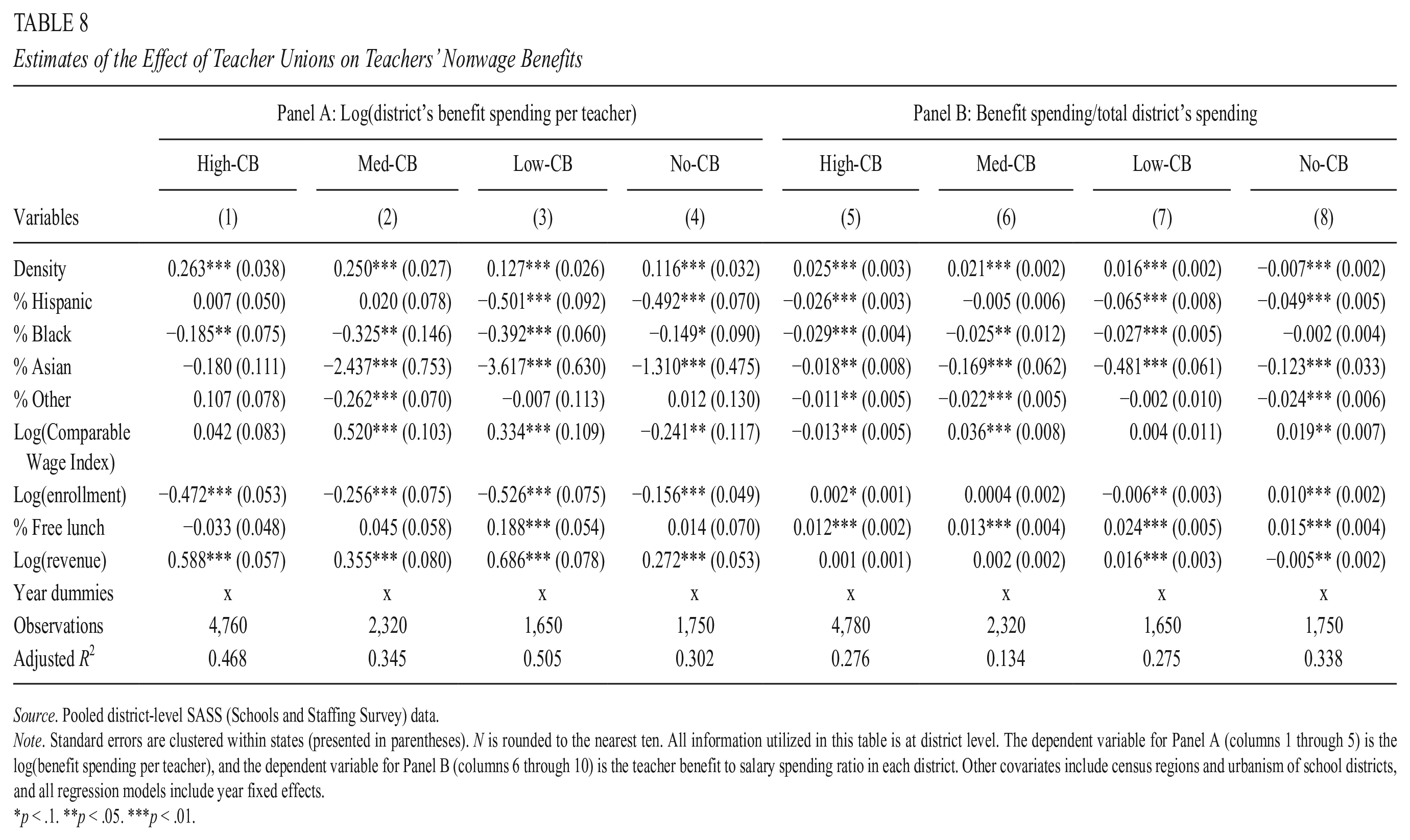
Both the multilevel model and PSM show that the union effects on teacher outcomes are relatively minor in the Med-CB and Low-CB groups. One may wonder why teachers in these groups join unions. In this section, I investigate if unions provide other advantages for their members beyond salary and working conditions by looking at the relation between unions and teachers’ nonwage benefits. Table 8 presents the results for districts’ benefit expenditure per teacher in Panel A and the ratio of benefit-to-total expenditure in Panel B. The information on nonwage benefits is only available at the district level, so I use union density as a measure of teachers’ unionization.²¹

Table 8

Estimates of the Effect of Teacher Unions on Teachers’ Nonwage Benefits

	Panel A: Log(district’s benefit spending per teacher)				Panel B: Benefit spending/total district’s spending
	High-CB	Med-CB	Low-CB	No-CB	High-CB	Med-CB	Low-CB	No-CB
Variables	(1)	(2)	(3)	(4)	(5)	(6)	(7)	(8)
Density	0.263*** (0.038)	0.250*** (0.027)	0.127*** (0.026)	0.116*** (0.032)	0.025*** (0.003)	0.021*** (0.002)	0.016*** (0.002)	−0.007*** (0.002)
% Hispanic	0.007 (0.050)	0.020 (0.078)	−0.501*** (0.092)	−0.492*** (0.070)	−0.026*** (0.003)	−0.005 (0.006)	−0.065*** (0.008)	−0.049*** (0.005)
% Black	−0.185** (0.075)	−0.325** (0.146)	−0.392*** (0.060)	−0.149* (0.090)	−0.029*** (0.004)	−0.025** (0.012)	−0.027*** (0.005)	−0.002 (0.004)
% Asian	−0.180 (0.111)	−2.437*** (0.753)	−3.617*** (0.630)	−1.310*** (0.475)	−0.018** (0.008)	−0.169*** (0.062)	−0.481*** (0.061)	−0.123*** (0.033)
% Other	0.107 (0.078)	−0.262*** (0.070)	−0.007 (0.113)	0.012 (0.130)	−0.011** (0.005)	−0.022*** (0.005)	−0.002 (0.010)	−0.024*** (0.006)
Log(Comparable Wage Index)	0.042 (0.083)	0.520*** (0.103)	0.334*** (0.109)	−0.241** (0.117)	−0.013** (0.005)	0.036*** (0.008)	0.004 (0.011)	0.019** (0.007)
Log(enrollment)	−0.472*** (0.053)	−0.256*** (0.075)	−0.526*** (0.075)	−0.156*** (0.049)	0.002* (0.001)	0.0004 (0.002)	−0.006** (0.003)	0.010*** (0.002)
% Free lunch	−0.033 (0.048)	0.045 (0.058)	0.188*** (0.054)	0.014 (0.070)	0.012*** (0.002)	0.013*** (0.004)	0.024*** (0.005)	0.015*** (0.004)
Log(revenue)	0.588*** (0.057)	0.355*** (0.080)	0.686*** (0.078)	0.272*** (0.053)	0.001 (0.001)	0.002 (0.002)	0.016*** (0.003)	−0.005** (0.002)
Year dummies	x	x	x	x	x	x	x	x
Observations	4,760	2,320	1,650	1,750	4,780	2,320	1,650	1,750
Adjusted R²	0.468	0.345	0.505	0.302	0.276	0.134	0.275	0.338

Source. Pooled district-level SASS (Schools and Staffing Survey) data.

Note. Standard errors are clustered within states (presented in parentheses). N is rounded to the nearest ten. All information utilized in this table is at district level. The dependent variable for Panel A (columns 1 through 5) is the log(benefit spending per teacher), and the dependent variable for Panel B (columns 6 through 10) is the teacher benefit to salary spending ratio in each district. Other covariates include census regions and urbanism of school districts, and all regression models include year fixed effects.

p < .1. **p < .05. ***p < .01.

Overall, the results show that unions are strongly associated with greater nonwage benefits of teachers. The magnitude of the association between union density and benefits per teacher is highest in the High-CB group and second highest in the Med-CB group. Column (1) shows that a 10% increase in union density is associated with 2.6% higher benefits per teacher in the High-CB group. This association is about half in the Low-CB group, as illustrated in column (3). Union density is also positively associated with benefits per teacher in the No-CB group.

Panel B shows that union density is positively associated with benefit-to-total spending ratio, and the association is highest in the High-CB group and second highest in the Med-CB group. Column (6) shows that a 10% increase in union density is associated with a 0.2% higher benefit-to-total spending ratio in the Med-CB group. In column (7), union density is also positively associated with benefit-to-total spending ratio in the Low-CB group. This suggests that teachers unions in the Med-CB and Low-CB groups tend to focus more on bringing higher nonwage benefits, rather than raising pay level. However, union density is negatively associated with benefit-to-total spending ratio in the No-CB group, implying that teachers unions in this group emphasize pay level more than benefits.

The Effect of Restricting Teachers’ Bargaining Rights on Teacher Outcomes

The group analysis reveals that there exists the substantial heterogeneity in union effects, and the legal environments in which unions operate play important roles in the magnitude of union influence. It also reveals that, to no surprise, the High-CB states provide the best compensation package and working conditions to their teachers. In this section, I exploit recent changes in state legislatures that compel Idaho, Indiana, Tennessee, and Wisconsin to move down toward lower tier groups, limiting the bargaining rights of public school teachers. The unanticipated legal changes in 2010–2011 in those four states form a natural experiment, allowing Freeman and Han (2015) to estimate the causal effect of the legal changes on unionism. They find that the new regulations dramatically reduced public school teachers’ bargaining coverage by 24 percentage points and union density by 11 percentage points.

Building on their studies, I estimate the effect of weakening unionism on teachers’ well-being. All the four states mandated CB before the passage of new state legislation, but their new laws no longer require districts to bargain with unions. Thus, I employ the DID estimation, using these four states as a treatment group and the remaining states in the High-CB and Med-CB groups with compulsory CB laws as a control group. Appendix D (online) presents the testing of the parallel-trend assumption of the DID model.

In demonstrating in previous sections that unions increase teacher compensation and improve working conditions, I anticipate that the legal change limiting unions’ negotiating power will reduce teachers’ well-being. Table 9 presents the results from the DID estimation in four panels. Panel A presents the base salary of the treatment and control groups before and after the legal changes. Teacher salaries rise in 2011–2012 compared with previous years in both groups (as salaries are often indexed to inflation), but the extent of the pay increase of the treatment group is about half that of the control group’s pay increase. The DID estimator shows that the change in public policy weakening unionism significantly reduces teacher salaries by 8.8%.

Table 9

The Effect of Legal Changes Limiting Collective Bargaining of Teachers on Teacher Compensation and Working Conditions

	Before legal changes	After legal changes	Treatment effect = After − Before
Panel A: Log(base salaries)
Treatment group	10.608 (0.006)	10.699 (0.009)	0.091 (0.006)
Control group	10.644 (0.004)	10.823 (0.005)	0.179 (0.006)
Difference (= Treatment − Control)	−0.036 (0.007)	−0.123 (0.011)	−0.088*** (0.024)
Panel B: Log(required hours)
Treatment group	3.292 (0.004)	3.369 (0.007)	0.077 (0.008)
Control group	3.278 (0.010)	3.362 (0.009)	0.084 (0.014)
Difference (= Treatment − Control)	0.014 (0.011)	0.007 (0.012)	0.007 (0.019)
Panel C: Log(benefit spending per teacher)
Treatment group	9.890 (0.017)	10.117 (0.023)	0.226 (0.028)
Control group	9.313 (0.057)	10.007 (0.052)	0.694 (0.078)
Difference (= Treatment − Control)	0.577 (0.060)	0.110 (0.057)	−0.467*** (0.164)
Panel D: Benefit spending/total spending
Treatment group	0.142 (0.001)	0.153 (0.002)	0.011 (0.003)
Control group	0.103 (0.003)	0.138 (0.004)	0.035 (0.005)
Difference (= Treatment − Control)	0.039 (0.004)	0.015 (0.004)	−0.024*** (0.012)

Source. The data sources are the pooled district–teacher matched SASS (Schools and Staffing Survey) data for Panels A and B and the pooled district-level SASS data for Panels C and D.

Note. Standard errors are clustered within states (presented in parentheses). The treatment group includes Wisconsin, Idaho, Indiana, and Tennessee. The control group includes other states in the High-CB and Med-CB groups that have mandatory collective bargaining laws. I do not estimate the difference-in-difference for contract days because the information on number of contract days is not available in the 2003–2004 SASS data.

p < .1. **p < .05. ***p < .01.

Panel B shows the required working hours for the treatment and control groups. The legal change has no significant effect on working conditions if measured by required working hours. Considering that the base salary falls by about 9%, this finding implies that the average hourly wage of teachers also falls by 9% after the legal change.

I present the estimated DID results for average benefit spending per teacher in Panel C. The data show that districts spend significantly less on nonwage benefits for teachers, following the legal changes. The increase in benefit spending per teacher in the treatment group is only about a third of that of the control group, leading to a significantly negative DID estimator.

Panel D reports the DID results for the benefit-to-total spending ratio. The increase in the benefit-to-total spending ratio in the control group is three times that of the treatment group.

The legal changes reduce districts’ benefit expenditure relative to total spending by 2.4%. Appendix E (online) presents the robustness and sensitivity checks of the DID results.

In sum, teachers unions have multiple potential pathways for improving teachers’ well-being beyond salary. If unions do not raise salaries, they may improve working conditions or increase nonwage benefits. CB is neither a necessary nor a sufficient condition for unions to affect teachers’ work lives: Teachers in CB districts do not necessarily earn higher pay than teachers in NA districts in some legal environments, and teachers unionize even where CB is prohibited, gaining a modest wage premium. The natural experiment occurring in four states nevertheless confirms that the general legal environments toward the CB of public school teachers play a critical role in unions’ influence on teachers’ well-being.

Discussion and Conclusion

This study examines the relationship between teachers unions and teachers well-being under different legal institutions for U.S. public school teachers. The significant contributions of this study to literature on teachers unions include the diverse measurements of unionism using nationally representative district–teacher matched data, the controls for both district-specific and teacher-specific demographics, the usage of a natural experiment to identify causal effects of unions, and the examination of union effects in the absence of CB.

The findings of this study lead to several implications for education policies. First, this study shows that about half of public school teachers still join unions, even when CB is prohibited, and that teachers unions can influence teacher outcomes, even if they are deprived of bargaining rights. Therefore, focusing on CB will underestimate unions’ roles in educational systems. Union membership can be a powerful mechanism for unions because membership rates represent the strength of the collective “voice” of teachers within their districts.

Second, teachers in districts whose legal institutions are favorable for unions enjoy substantially better working lives, but simply permitting bargaining contracts without an ability to collect union dues from nonunion teachers does not guarantee better economic conditions for teachers. Both the Med-CB and Low-CB groups allow CB, but their union effects, on average, are often smaller than the union effects in the No-CB group that bans CB. The free rider problems in these two middle groups reduce unions’ financial stability, limiting their capability of negotiating better terms and conditions for teachers. Moreover, the natural experiments in four states show that legal changes leading toward more hostile institutions for teachers unions make negative impacts on teacher outcomes. Hence, this research predicts that the Janus decision and the recent movement toward right-to-work laws in several states, including Kentucky and Michigan, will significantly weaken the union effects on teachers’ well-being.

Third, the lower pay, poor working conditions, and fewer nonwage benefits provided in districts with weak unions may decrease average teacher quality. Due to the unpopularity of the teaching profession, it is difficult to attract and retain high-quality teaching applicants. This study suggests that strong teachers unions, by improving compensation and working conditions, are able to reduce teacher attrition and increase teacher quality.²²

Finally, the union effects and the mechanisms through which unions affect teacher outcomes vary in different legal environments. For instance, unions in the Med-CB and Low-CB groups have small effects on teacher pay, but they significantly raise the nonwage benefits each teacher receives. This finding suggests that the external validity of experimental studies on union effects in limited geographic areas will be weak.

In the debate over public sector unions, both the pro-union and anti-union parties seem to believe that CB is the be-all and end-all for public sector workers. This study rejects that proposition. The legal institutions for CB are important for teachers unions to influence teachers’ working lives, but unions organize with or without bargaining power, as “freedom of assembly” asserts. Furthermore, CB is neither necessary nor sufficient for teachers unions to affect teachers’ work lives, and meet and confer or higher union membership can improve teacher outcomes in the absence of CB. This research provides valuable information for understanding the role of teachers unions in the post-Janus period. Teachers unions will evolve to find ways to enhance teachers’ well-being even in the most hostile legal environments. Therefore, broadening the perspective toward unionism beyond CB is essential to fully understand how unions behave and operate in the U.S. education sector.

Supplemental Material

DS_10.1177_2332858419867291 – Supplemental material for The Impact of Teachers Unions on Teachers’ Well-Being Under Various Legal Institutions: Evidence From District–Teacher Matched Data

Supplemental material, DS_10.1177_2332858419867291 for The Impact of Teachers Unions on Teachers’ Well-Being Under Various Legal Institutions: Evidence From District–Teacher Matched Data by Eunice S. Han in AERA Open

Footnotes

Acknowledgements

I thank Elaine Bernard, Raj Chetty, Richard Freeman, Jeffrey Keefe, Jerry Marschke, Marty West, seminar participants at Harvard University and Brigham Young University, and colleagues at the University of Utah for their many helpful comments. I thank the National Bureau of Economic Research (NBER) for providing me with the necessary facilities and assistance. I also thank the National Center for Educational Statistics (NCES) for kindly providing me with the data. The views expressed herein are my own and do not necessarily reflect the views of the NBER or the NCES.

ORCID iD

Eunice S. Han

Notes

Author

EUNICE S. HAN is an assistant professor at the University of Utah, a senior research associate at the Labor and Worklife Program at Harvard Law School, and a research associate at Economic Policy Institute. Han’s recent research focuses on the impact of unionism on the local labor market, especially on income inequality and on economic mobility.

References

Abood v. Detroit Board of Education, 431 U.S. 209 (1977).

Arnesen

(2007). Encyclopedia of U.S. labor and working-class history (Vol. 1). New York, NY: Routledge.

Baron

E. J.

(2018). The effect of teachers’ unions on student achievement in the short run: Evidence from Wisconsin’s Act 10. Economics of Education Review, 67, 40–57.

Baugh

Stone

(1982). Teachers, unions, and wages in the 1970s: Unionism now pays. Industrial and Labor Relations Review, 35, 368–376.

Belman

Heywood

J. D.

Lund

(1997). Public sector earnings and the extent of unionization. Industrial and Labor Relations Review, 50, 610–628.

Brunner

E. J.

Squires

(2013). The bargaining power of teachers’ unions and the allocation of school resources. Journal of Urban Economics, 76, 15–27.

Budd

J. W.

(2007). The effect of unions on employee benefits and nonwage compensation: Monopoly power, collective voice, and facilitation. In Bennett

J. T.

Kaufman

B. E.

(Eds.), What do unions do? A twenty-year perspective (pp. 160–192). Piscataway, NJ: Transaction.

Delaney

J. T.

(1985). Unionism, bargaining spillovers, and teacher compensation. In Lipsky

D. B.

(Eds.), Advances in industrial relations 2 (pp. 111–142). Greenwich, CT: JAI Press.

Eberts

R. W.

Stone

J. A.

(1984). Unions and public schools: The effect of collective bargaining on American Education. Lexington, MA: Lexington Books.

10.

Eberts

R. W.

Stone

J. A.

(1985). Communications: Wages, fringe benefits, and working conditions: An analysis of compensating differentials. Southern Economic Journal, 52, 274–279.

11.

Ehrenberg

R. G.

Schwarz

J. L.

(1986). Public sector labor markets. In Ashenfelter

O. C.

Layard

(Eds.), Handbook of labor economics 2 (pp. 1219–1268). Amsterdam, Netherlands: North-Holland.

12.

Farber

H. S.

(1984). Right-to-work laws and the extent of unionization. Journal of Labor Economics, 2, 319–352.

13.

Frandsen

(2016). The effects of collective bargaining rights on public employee compensation: Evidence from teachers, firefighters, and police. Industrial and Labor Relations Review, 69, 84–112.

14.

Freeman

R. B.

(1984). Longitudinal analyses of the effects of trade unions. Journal of Labor Economics, 2, 1–26.

15.

Freeman

R. B.

(1985). Unions, pensions, and union pension funds. In Wise

D. A.

(Ed.), Pensions, labor, and individual choice (pp. 89–121). Chicago, IL: University of Chicago Press.

16.

Freeman

R. B.

(1986). Unionism comes to the public sector. Journal of Economic Literature, 24, 41–86.

17.

Freeman

R. B.

Han

E. S.

(2015). When states restrict public sector bargaining rights (Working Paper).

18.

Freeman

R. B.

Ichniowski

(Eds.). (1988). When public sector workers unionize. Chicago, IL: University of Chicago Press.

19.

Freeman

R. B.

Medoff

J. L.

(1984). What do unions do? New York, NY: Basic Books.

20.

Freeman

R. B.

Valletta

(1988). NBER public sector collective bargaining law dataset. In Freeman

Ichniowski

(Eds.), When public sector workers unionize. Chicago, IL: University of Chicago Press.

21.

Gyourko

Tracy

(1991). Public sector bargaining and the local budgetary process. Research in Labor Economics, 12, 117–136.

22.

Han

E. S.

(2017). The myth of unions’ overprotection of bad teachers: Evidence from the district–teacher matched data on teacher turnover (Working Paper Series, Labor and Worklife Program). Cambridge, MA: Harvard Law School.

23.

Hirsch

B. T.

Macpherson

D. A.

DuMond

J. M.

(1997). Workers’ compensation recipiency in union and nonunion workplaces. Industrial and Labor Relations Review, 50, 213–236.

24.

Hirsch

B. T.

Macpherson

D. A.

Winters

J. V.

(2011, March). Teacher salaries, state collective bargaining laws, and union coverage. Paper presented at the annual conference of the Association for Education Finance and Policy, Seattle, WA.

25.

Hoxby

C. M.

(1996). How teachers’ unions affect education production. Quarterly Journal of Economics, 111, 671–718.

26.

Lemke

R. J.

(2004). Estimating the union wage effect for public school teachers when all teachers are unionized. Easter Economic Journal, 30, 273-291.

27.

Lewis

H. G.

(1986). Union relative wage effects. In Ashenfelter

O. C.

Layard

(Eds.), Handbook of labor economics (Vol. 2, pp. 1139–1181). Amsterdam, Netherlands: Elsevier.

28.

Lipsky

D. B.

(1982). The effect of collective bargaining on teacher pay: A review of the evidence. Educational Administration Quarterly, 18(1), 14–42.

29.

Lovenheim

M. F.

(2009). The effect of teachers’ unions on education production: Evidence from union election certifications in three Midwestern states. Journal of Labor Economics, 27, 525–587.

30.

Martin

Rence

(1984). Vertical spillovers, market concentration, union coverage, and wages. Journal of Labor Research, 5, 177–189.

31.

Moe

T. M.

(2011). Special interest. Washington, DC: Brookings Institution Press.

32.

Mykerezi

West

(2011). Teachers’ unions and compensation: The impact of collective bargaining on salary schedules and performance pay schemes. Economics of Education Review, 30, 99–108.

33.

National Center for Education Statistics. State nonfiscal survey of public elementary/secondary education for 2011–2012. Washington, DC: U.S. Department of Education.

34.

Podgursky

M. J.

(2003). Fringe benefits: There is more to compensation than a teacher’s salary. Education Next, 3, 71–76.

35.

Rose

Sonstelie

(2010). School board politics, school district size, and the bargaining power of teachers’ unions. Journal of Urban Economics, 67, 438–450.

36.

Rosen

(1969). Trade union power, threat effects and the extent of organization. Review of Economic Studies, 36, 185–196.

37.

Rosenbaum

P. R.

Rubin

D. B.

(1985). Constructing a comparison group using multivariate matched sampling methods that incorporate the propensity score. The American Statistician, 39, 33–38.

38.

Taylor

L. L.

Fowler

W. J.

(2006). A comparable wage approach to geographic cost adjustment. Washington, DC: National Center for Education Statistics.

39.

West

K. L.

(2015). Teachers’ unions, compensation, and tenure. Industrial Relations: A Journal of Economy and Society, 54, 294–320.

40.

Winters

J. V.

(2011). Teacher salaries and teacher unions: A spatial econometric approach. Industrial and Labor Relations Review, 64, 747–764.

41.

Zwerling

H. L.

Thomason

(1995). Collective bargaining and the determinants of teachers’ salaries. Journal of Labor Research, 16, 467–484.

Supplementary Material

Please find the following supplemental material available below.

For Open Access articles published under a Creative Commons License, all supplemental material carries the same license as the article it is associated with.

For non-Open Access articles published, all supplemental material carries a non-exclusive license, and permission requests for re-use of supplemental material or any part of supplemental material shall be sent directly to the copyright owner as specified in the copyright notice associated with the article.

0.00 MB

0.48 MB