Sage Journals: Discover world-class research

Abstract

Binaural hearing can improve the intelligibility of a speech source spatially separated from competing sound sources when compared to co-located conditions. Monaural speech intelligibility models cannot predict this spatial release from masking. A binaural front end is proposed that can be combined with monaural models to do so. From the noisy speech signals at the two ears, it produces binaurally-enhanced monaural signals that can be evaluated by monaural models. A stationary and a time-dependent version of the front end were tested here with the monaural Hearing Aid Speech Perception Index (HASPI) that compares the envelope modulations of the noisy speech to those of the clean speech. The model predictions were compared to the intelligibility scores of three datasets collected with normal-hearing listeners via headphones measurements in anechoic conditions. A stationary speech-shaped noise (SSN) was tested at 10 azimuths in dataset 1. In dataset 2, an SSN or a non-stationary noise were tested at three azimuths, with or without ideal binary mask processing. In dataset 3, the competing sounds were obtained by mixing the signals from an SSN co-located with the target speech, a diffuse noise coming from all directions, and a spatially-separated SSN. The stationary-front-end predictions are very accurate in the conditions with a spatially-separated SSN, while monaural HASPI predictions at the ear with the better signal-to-noise ratio under-estimate intelligibility. The front-end predictions are slightly less accurate for non-stationary noise but under-estimate intelligibility with diffuse noise. The time-dependent version of the front end systematically over-estimates intelligibility at low signal-to-noise ratios.

Keywords

speech intelligibility binaural hearing auditory models

Introduction

Binaural hearing improves speech intelligibility in noise as it allows for spatial release from masking: when a speech target and a masking sound source are at the same position, the target is less intelligible than when the masking source is moved to a different direction (Hawley et al., 2004; Plomp, 1976). The gain in intelligibility, or release from masking, is thought to be based on two binaural mechanisms (Bronkhorst & Plomp, 1988; Culling & Lavandier, 2021): (a) better-ear listening, which relies on the ear having a better signal-to-noise ratio (SNR) due to the interaural level difference (ILD) created by the acoustic shadow of the head, so that the listener can use this ear to better understand the target; (b) binaural unmasking, which relies on the differences in interaural time difference (ITD) produced by the two sources. Following the Equalization-Cancellation theory (Durlach, 1972), the auditory system would be able to cancel to some extent the noise if it has an ITD different from that of the speech. It would do that by first by equalizing the signals at the ears (applying a gain and a delay to compensate for the noise ITD and ILD) and then subtracting the signals at one ear from the other to cancel the noise. Several binaural speech intelligibility models have been proposed to predict these effects (for a review, see Lavandier & Best, 2020), but monaural speech intelligibility models cannot do so. The aim of the present study was to test a model front end that can be combined with monaural models to predict the influence of binaural hearing on speech intelligibility.

From the binaural signals at the ears, the front end produces binaurally enhanced monaural signals on which monaural models can be used. The idea of re-synthetizing binaurally-enhanced signals is inspired from the model of Beutelmann and Brand (2006). The front-end implementation is based on the modified binaural short-time objective intelligibility index (MBSTOI; Andersen et al., 2018). Like MBSTOI, the front end takes as inputs the noisy speech signal at the two ears along with a clean version of the same speech, also at the two ears. The clean speech is used as a reference. The front-end outputs are binaurally-enhanced monaural versions of the noisy and clean speech. The front end was tested here in combination with the monaural Hearing Aid Speech Perception Index (HASPI; Kates and Arehart, 2021), that also uses the noisy and clean speech as inputs.

Because binaural speech intelligibility models have already been proposed in the literature, one might wonder whether the proposed front end would still be useful. First, several of these binaural models are SNR-based (Beutelmann et al., 2010; Beutelmann & Brand, 2006; Collin & Lavandier, 2013; Cueille & Lavandier, 2025; Lavandier & Culling, 2010; Leclère et al., 2015; Rennies et al., 2011; Tang et al., 2016; Vicente et al., 2020; Wan et al., 2010). SNR-based models require as inputs the speech and noise signals separately. It is in particular the case for the model front end of Beutelmann and Brand (2006) that inspired the present study. Considering the speech and noise separately might not be the most appropriate when one wants to consider nonlinearly processed noisy speech (such as in hearing aid applications). The nonlinear processing is different when it is applied to the noise and speech separately rather than to the noisy speech. The model of Cosentino et al. (2014) uses directly the noisy speech, but it works only for frontal speech in the presence of a single noise source. In a similar way, the model of Mi and Colburn (2016) requires a priori knowledge of the speech direction. The binaural version of the speech transmission index (STI; Wijngaarden & Drullman, 2008) assumes that the speech is the only source of modulations in the signals in order to identify its direction, and it was not tested for modulated maskers. Another modulation-based model proposed by Chabot-Leclerc et al. (2016) has been shown to largely overestimate spatial release from masking (Andersen et al., 2018), leading to large prediction errors compared to its monaural version (Jørgensen et al., 2013), which might benefit from a different binaural front end. Several binaural models based on machine learning have also been proposed recently (Barker et al., 2022; Josupeit & Hohmann, 2017; Schädler et al., 2018), but the most accurate of these models require prior training with speech and conditions very similar to the evaluation material. Among the correlation-based models, MBSTOI can be used only for normal-hearing (NH) listeners (Andersen et al., 2018). HASPI can handle hearing impairment (Kates and Arehart, 2021), but it is monaural and would require either to be revised to directly incorporate aspects of binaural processing, as tested in parallel to the present study by Kates, Lavandier, Arehart, et al. (2025), or to be used with a binaural front end. Such a front end was proposed by Hauth et al. (2020), who tested it in combination with an SNR-based monaural model. Like the binaural STI, this front end cannot be used in conditions where the masking sound contains speech-like modulations. The availability of a model's specific inputs and the applicability of its underlying assumptions will determine its usability in practice for any given application (Lavandier & Best, 2020). The variety of applications makes for the variety of models.

The front end proposed here was combined with HASPI and tested using three datasets from Andersen et al. (2018): intelligibility scores measured with headphones at different SNRs for NH listeners and a Danish speech source simulated in anechoic conditions in front of the listener. In dataset 1 (D1), a stationary speech-shaped noise (SSN) was simulated at one of 10 azimuths. In dataset 2 (D2), an SSN or a non-stationary noise was simulated at one of three azimuths, with or without nonlinear processing simulating noise reduction in hearing aids. In dataset 3 (D3), the competing sounds were obtained by mixing a diffuse noise with an SSN simulated co-located with or spatially-separated from the target speech. This study is a first step in the development of the front end, comparing different front-end versions on a limited set of data chosen to test specifically what the front end was developed to handle: very clear binaural effects (D1, D3), combined with an example of non-stationary masker and of nonlinear processing (D2). In particular, at this stage, the front end was not tested for hearing-impaired (HI) listeners nor reverberation.

Models

Two versions of binaural front end, stationary and time-dependent, were tested in combination with monaural HASPI v2 (Kates & Arehart, 2021), which was re-fitted here to be applied to the Danish intelligibility datasets (Andersen et al., 2018).

Monaural HASPI v2

HASPI v2 is a correlation model that compares the noisy speech signal to a clean version of the same speech used as a reference (Kates and Arehart, 2021). The signals are passed through a model of the auditory periphery that computes the envelope in each frequency band. A time-frequency modulation analysis is then performed and the noisy speech envelopes are cross-correlated with the clean speech envelopes, producing a correlation value at each of 10 modulation frequencies. These 10 correlations are then mapped to a single HASPI value corresponding to the predicted proportion sentence correct. This mapping is done through a set of 10 neural networks, averaging the outputs of these networks to improve immunity to overfitting.

HASPI v2 has been described in detail by Kates and Arehart (2021, 2022), so only an overview is provided here. The model of the auditory periphery starts with re-sampling the signals to 24 kHz, followed by a broadband temporal alignment of the noisy speech to the clean speech reference. A second temporal alignment stage is later provided within each frequency band. Note that these two temporal alignment steps were bypassed in the present study, because the signals considered were already perfectly time-aligned when they were synthesized (Andersen et al., 2018). The peripheral model can be adjusted in response to the listener's audiogram, making HASPI v2 appropriate for both NH and HI listeners. Here, only NH data were considered, so the model of the normal auditory periphery was used for all signals (assuming a flat audiogram at 0 dB HL). After re-sampling, the signals are passed through a middle ear filter (Kates, 1991), followed by a fourth-order gammatone filterbank (Patterson et al., 1995); with 32 filters spanning the frequency range from 80 to 8,000 Hz, the bandwidth of each filter increasing with increasing signal level above 50 dB SPL (Baker & Rosen, 2002, 2006). Dynamic-range compression is applied to the output of each filter to mimic the gain variations provided by the outer hair cell behavior. Linear amplification is applied to inputs below 30 or above 100 dB SPL, while amplitude compression is applied to signals lying between 30 and 100 dB SPL. The envelopes are then converted to dB re: auditory threshold (dB SL), sound levels below threshold being set to 0 dB SL. Inner hair cell adaptation is applied to the envelope dB output using a rapid time constant of 2 ms and a short-term time constant of 60 ms (Harris & Dallos, 1979). Compensation is then provided for the auditory filter delays (Wojtczak et al., 2010).

For the envelope modulation analysis, the dB SL envelopes are lowpass filtered at 320 Hz using a linear-phase filter having a raised-cosine impulse response (to prevent negative envelope values), and subsampled at 2,560 Hz (8 times the lowpass filter cutoff frequency). At each time sample, the envelope values (in dB) in the 32 frequency bands correspond to a log spectrum on an auditory frequency scale. These spectra are fitted with five basis functions ranging from ½ cycle per spectrum to 2½ cycles per spectrum. The basis filter functions correspond to both Mel-frequency cepstral coefficients (Mitra et al., 2012) and the principal components of speech short-time spectra (Zahorian & Rothenberg, 1981). The five sequences of cepstral coefficients are passed through a 10-filter modulation filterbank with center frequencies ranging from 2 to 256 Hz, and 1.5-Q filters consistent with values resulting from fitting amplitude modulation discrimination data (Ewert et al., 2002; Ewert & Dau, 2000). This produces a total of 50 output envelope sequences. The noisy speech and clean speech reference envelopes are compared using cross-covariance. Because the basis function cross-correlations are similar to one another (Kates & Arehart, 2015), the cross-covariance functions are averaged over the five basis functions, resulting in 10 correlations, one per envelope modulation filter.

The final processing stage of HASPI v2 is an ensemble of 10 neural networks that map the 10 averaged envelope correlations to the intelligibility scores. Each neural network has 10 inputs, a hidden layer with four neurons, and a single-neuron output layer, using a sigmoid activation function for all layers. Ensemble averaging is used to reduce the possibility of overfitting the data.

Monaural HASPI v2 Re-fitting

In HASPI v2, the neural networks were trained using monaural English sentence correct scores measured at positive SNRs (Kates & Arehart, 2021). They associate envelope correlations at positive SNRs with full-sentence correct scores. In this paper, HASPI was used to predict binaural Danish word correct scores measured at very low SNRs (Andersen et al., 2018), much lower than the SNRs for which HASPI v2 was designed. In a given condition, understanding a full sentence correctly is much more difficult than getting single words right, and sentence correct scores will differ from word correct scores (Kates, 2023). So here, the neural network ensemble had to be re-designed to associate envelope correlations at negative SNRs with word correct scores. In our modeling framework, the aim of the neural networks is not to model binaural processing (which is done by the front end). Thus, the training of the 10 networks was based on monaural HASPI values computed at one ear in conditions with no binaural effects involved.

The training data was composed of the individual data from the co-located conditions of the three datasets D1, D2 and D3 considered in the present study and measured by Andersen et al. (2018). These conditions are described in details below in the section “Datasets and predictions.” They all use the same Danish speech material but involved different listeners at many different SNRs, along with different types of noise and nonlinear processing. There is one co-located condition in D1, one in D3, and three in D2. These five conditions were not all measured with the same number of SNRs and listeners (but always with three experimental repetitions). The neural network weights depend on the relative proportion of each condition in the training data. The data representation was weighted to give the same weight to each of the five co-located conditions by replicating 42 times the co-located data of D1, 30 times the co-located data of D2, and 39 times the co-located data of D3, leading to about 2,500 “training vectors” per condition, 12,576 vectors in total. Each of these vectors contained the individual word correct score (averaged across the three repetitions in the experiment) and the 10 envelope correlations resulting from applying monaural HASPI v2 to the left ear signals (the right ear signals were very similar for these anechoic conditions with frontal speech and noise), with the reference clean speech signals calibrated at 65 dB SPL and the noisy speech signals calibrated at their presentation level during the experiment (see section Implementation and evaluation of the models below), concatenating the signals used for the different listeners and the three experimental repetitions after trimming them from any silent portion at their beginning and end.

The fitting procedure followed the one used for HASPI v2 (Kates & Arehart, 2021). The 10 networks were initialized to different sets of random weights, and network training used backpropagation with a mean-squared error loss function (Rumelhart et al., 1986). The network outputs were combined using bootstrap aggregation (Breiman, 1996). The training of each network used a subset of the 12,576 training vectors, each subset being selected with replacement and comprising (1 – 1/e) = 0.632 of the available training data. Each network was trained on 5,000 iterations of its randomly selected training subset. The main benefits of bootstrap aggregation in reducing overfitting are obtained for an ensemble of 10 neural networks (Breiman, 1996; Hansen & Salamon, 1990).

The difference in the neural network ensemble used here compared to HASPI v2 is that the networks have two neurons instead of four in their hidden layer. Originally, the same 4-neuron networks were tested, but they led to unexpected behavior of monaural HASPI in some conditions: non-monotonic variations with increasing SNR. The envelope correlations between clean and noisy speech do not decrease with increasing SNR. The occasional decreases of HASPI values with increasing SNR were associated with the neural networks probably overfitting the data in the new range of very low SNRs considered here, modeling the specific noise signals rather than providing a general solution for all noises. Reducing the number of neurons in the hidden layer eliminated the non-monotonic variations in the HASPI values. The simplest networks (with fewer degrees of freedom) still leading to the best fitting performance on the training data were the two-neuron networks. The quality of this fitting is highlighted by the very good description of the co-located (training) data by the monaural HASPI values computed at the better ear (dotted black lines) shown in Figures 1 ‒3.

Figure 1.

Mean proportion word correct with standard error across listeners and repetitions as a function of tested SNR for dataset D1. Each panel corresponds to a noise azimuth. The red symbols are the measured data, while the black lines are the predictions from the three model versions: monaural HASPI at the better ear (dotted line, “BE-only”), stationary front end with HASPI (full line, “front end”), time-dependent (non-stationary) front end with HASPI (dashed line, “non-stat front end”). The BE-only predictions in the co-located condition (“noise @ 0˚”) highlight the results of the HASPI v2 neural network re-fitting (see Models section).

Figure 2.

Mean proportion word correct with standard error across listeners and repetitions as a function of tested SNR for dataset D2. The left column corresponds to the masker at 20˚ (“S0N0”), the middle column to the masker at 0˚ (“S0N0,” co-located condition), the right column to the masker at −115˚ (“S0N-115”). The top row corresponds to the SSN with IBM processing (“SSN + IBM”), the middle row to the bottle (non-stationary) noise without IBM processing (“bottle”), the bottom row to the bottle noise with IBM processing (“bottle + IBM”). The red symbols are the measured data, while the black lines are the predictions from the three model versions: monaural HASPI at the better ear (dotted line, “BE-only”), stationary front end with HASPI (full line, “front end”), time-dependent (non-stationary) front end with HASPI (dashed line, “non-stat front end”). The BE-only predictions in the co-located conditions (middle column) highlight the results of the HASPI v2 neural network re-fitting (see Models section).

Figure 3.

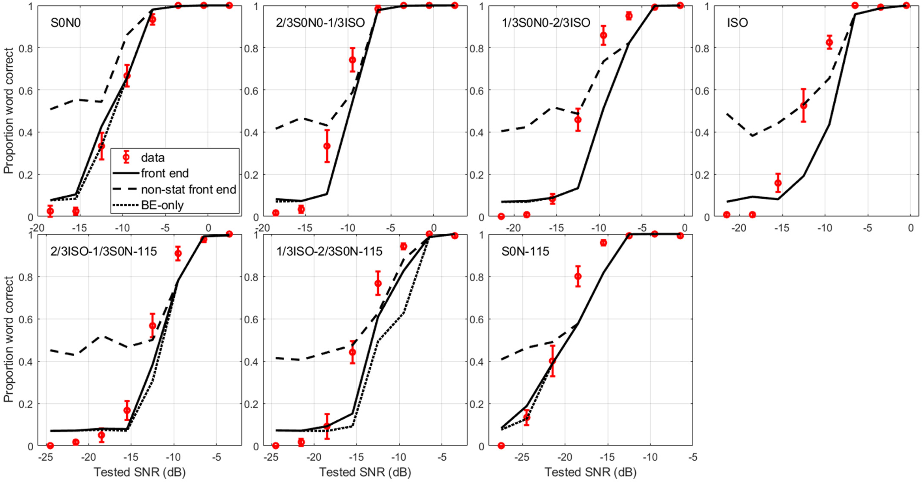
Mean proportion word correct with standard error across listeners and repetitions as a function of tested SNR for dataset D3. each panel corresponds to a condition for which the stationary noise was a mixture of co-located SSN at 0˚ (“S0N0”), spatially-separated SSN at −115˚ (“S0N-115”) and isotropic SSN (“ISO”). The top left panel is for a fully co-located SSN, the bottom right panel is for a fully spatially-separated SSN, and the top right panel is for a fully isotropic SSN. The red symbols are the measured data, while the black lines are the predictions from the three model versions: monaural HASPI at the better ear (dotted line, “BE-only”), stationary front end with HASPI (full line, “front end”), time-dependent (non-stationary) front end with HASPI (dashed line, “non-stat front end”). The BE-only predictions in the co-located condition (top left panel) highlight the results of the HASPI v2 neural network re-fitting (see Models section).

Once trained on the co-located data and monaural HASPI values, the neural network ensemble was kept constant, in particular the same ensemble was used with the binaural front ends and when considering spatially separated conditions involving binaural hearing.

Binaural Front Ends and Three Model Versions

Three model versions were compared in the present study: monaural HASPI computed at the better ear, a stationary binaural front end combined with HASPI, and a time-dependent (non-stationary) binaural front end combined with HASPI. All model versions use the same inputs: the clean and noisy speech signals at the two ears.

Better-ear (BE-Only) Version

The first model version computes the monaural HASPI values at the left ear, at the right ear, and selects the highest value of the two. It is a very crude better-ear solution, both broadband and long-term, because HASPI values are broadband and computed over the whole duration of the signals, so this model assumes that the better ear is better all the time at all frequencies. It is denoted as the better-ear (BE-only) model in the following.

Stationary Binaural Front end

From the binaural signals at the ears, the stationary front end produces binaurally-enhanced monaural signals (Beutelmann & Brand, 2006) on which monaural HASPI can be used. The front-end implementation is based on MBSTOI (Andersen et al., 2018).

MBSTOI predicts intelligibility by looking at the correlation between the envelopes of the clean and noisy speech signals, the same inputs as HASPI. After a time-frequency decomposition, an envelope correlation is computed at each ear. A direct implementation of equalization-cancellation (E-C; Durlach, 1972) is also used to combine the left and right signals (Beutelmann & Brand, 2006): applying delays and gains to the left-ear signal and subtracting it from the right-ear signal. The delay and gain are chosen to maximize an envelope-correlation-based objective function. This process is done independently for each time frame and frequency band, in which the best envelope correlation among the three correlation values computed on the left-ear, right-ear and E-C enhanced signals is selected. The selected values are averaged across time-frequency units to get an MBSTOI value that is then mapped to intelligibility ratings using a fitted logistic function.

The stationary front end is based on MBSTOI, but first, there is no time decomposition, it considers the signals over their entire duration. Then, instead of selecting the best envelope correlation in each frequency band, the corresponding signals (left-ear, right-ear, or E-C enhanced) are selected, and summed across frequency to reconstruct broadband binaurally-enhanced monaural signals (Beutelmann & Brand, 2006). This requires the signal waveforms so the front end is implemented in the time domain (while MBSTOI is implemented in the spectral domain).

The E-C stage adjusts the relative gains and time delays applied to the reference and noisy signals in each frequency band to maximize the MBSTOI objective function. The reference (clean speech) input signals at the left and right ears are here denoted as $x_{L} (n)$ and $x_{R} (n)$ , respectively, and the noisy signals are $y_{L} (n)$ and $y_{R} (n)$ . The first processing step is an auditory filterbank that comprises 16 channels, with center frequencies ranging from 80 to 8,000 Hz on an auditory critical band frequency scale. The lowest frequency band is provided by a lowpass filter and the highest band by a highpass filter, with the remaining bands given by bandpass filters. All filters are linear-phase with a filter duration of 16 ms at the sampling rate of 22.05 kHz.

Uncertainty is implemented in the E-C process (in the time domain) by applying jitters in amplitude and time into the signals used to determine the best E-C gains and delays. The amplitude and timing jitters are zero-mean Gaussians as specified by Wan et al. (2010). The amplitude jitter is multiplicative with a standard deviation of 0.25 and the timing jitter has a standard deviation of 105 μs, and these nominal values can be adjusted up or down by multiplication with a jitter gain. This jitter gain controls simultaneously the amount of amplitude and timing jitters. It constitutes the only free parameter of the binaural front end. The jitter is assumed to be independent in each frequency band, and is applied to both the reference and noisy signals. We define the amplitude jitter for the left and right ears in frequency band k as $ϵ_{L, k} (n)$ and $ϵ_{R, k} (n)$ , respectively, and define the timing jitters as $δ_{L, k} (n)$ and $δ_{R, k} (n)$ , with the timing jitters quantized to the nearest sample. The timing jitter is applied by resampling the input sequence at the jittered sample values, after which the amplitude jitter is applied by multiplying the resampled sequence by the amplitude jitter function. The jittered waveforms at the left and right ears are given by

{\hat{z}}_{L, k} (n) = [1 + ϵ_{L, k} (n)] z_{L, k} (n - δ_{L, k} (n))

{\hat{z}}_{R, k} (n) = [1 + ϵ_{R, k} (n)] z_{R, k} (n - δ_{R, k} (n))

(1)

where equation (1) is applied to both the reference and noisy signals (i.e.,

z

represents

x

and

y

The signal envelopes are extracted using a stepped raised cosine (von Hann) window. The window duration is set to 25.6 ms to match the short-time FFT window size used in MBSTOI (Andersen et al., 2018). The window step size is half its duration, so the envelope subsampling rate is 78.125 Hz. Each windowed output sample is computed as the RMS sum of the waveform over the windowed segment.

The MBSTOI objective function is a modified envelope correlation computed from the signal envelopes. It is an updated objective function compared to a previous version of MBSTOI (Andersen et al., 2016), modified to eliminate a prediction bias at low SNRs for spatially distributed maskers. Three objective function values are computed and compared for each frequency band. They are computed using the signals on the left ear alone, on the right ear alone, and on both ears using the E-C process. The left- and right-ear objective functions are computed with the envelopes of the reference and noisy signals with no jitter applied. Consider, for example, the left ear signals. The mean is removed from the reference and noisy signal envelopes, giving vectors of zero-mean envelope samples $x_{L, k}$ and $y_{L, k}$ in each frequency band. The objective function is equation (26) from Andersen et al. (2018):

g_{L, k} = \sqrt{\frac{E [x_{L, k}^{T} x_{L, k}]}{E [y_{L, k}^{T} y_{L, k}]}}

(2)

where

E [.]

is the expectation operator. The objective function for the right ear alone is computed in a similar fashion using the right ear reference and noisy signal envelopes.

The objective function calculation for the E-C process uses differences between the left- and right-ear jittered signals. When defining $γ_{k}$ as the gain applied to the left ear signals in band k (the inverse gain being applied to the right ear signals) and $μ_{k}$ as the time delay in samples applied between the left and right ear signals, the difference between the left and right ear reference signals and the difference between the noisy signals are given by

{\tilde{x}}_{k} (n) = γ_{k} {\hat{x}}_{L, k} (n - μ_{k} / 2) - \frac{1}{γ_{k}} {\hat{x}}_{R, k} (n + μ_{k} / 2)

{\tilde{y}}_{k} (n) = γ_{k} {\hat{y}}_{L, k} (n - μ_{k} / 2) - \frac{1}{γ_{k}} {\hat{y}}_{R, k} (n + μ_{k} / 2)

(3)

A grid search is used to find the values of $γ_{k}$ and $μ_{k}$ that maximize the envelope-based objective function given by equation (2) applied to ${\tilde{x}}_{k}$ and ${\tilde{y}}_{k}$ , with separate searches in each frequency band. The gain $γ_{k}$ is varied such that $20 l o g_{10} (γ_{k})$ goes from −20 to 20 dB in 10 equal 4-dB steps, and the time delay $μ_{k}$ goes from −1 to 1 ms in 25 equal 0.08-ms steps.

In each frequency band k, the three objective function values, left-ear, right-ear and E-C, are compared. If the left ear objective function is greatest, the left ear gain $γ_{k}$ = 1 and the right ear gain = 0 (thus selecting the left-ear signals). Similarly, if the right ear objective function is greatest, the left ear gain = 0 and the right ear gain = 1. If the E-C objective function is greatest, the values of $γ_{k}$ and $μ_{k}$ that correspond to this maximum are saved. These gain and delay values are then used to combine the left and right ear signals without jitters to provide E-C processed monaural signals. If the left ear had the highest objective function, the combined reference signal in that frequency band is given by ${\overset{˘}{x}}_{k} (n) = x_{L, k} (n)$ and the degraded signal is given by ${\overset{˘}{y}}_{k} (n) = y_{L, k} (n)$ . Similarly, if the right ear had the highest objective function, the combined reference signal in that frequency band is given by ${\overset{˘}{x}}_{k} (n) = x_{R, k} (n)$ and the degraded signal is given by ${\overset{˘}{y}}_{k} (n) = y_{R, k} (n)$ . If the E-C process returned the highest objective function, then the corresponding left and right gains and delays in the frequency band are applied to the unjittered reference and degraded signals and their left/right difference is computed as the selected signals:

{\overset{˘}{x}}_{k} (n) = γ_{k} x_{L, k} (n - μ_{k} / 2) - \frac{1}{γ_{k}} x_{R, k} (n + μ_{k} / 2)

{\overset{˘}{y}}_{k} (n) = γ_{k} y_{L, k} (n - μ_{k} / 2) - \frac{1}{γ_{k}} y_{R, k} (n + μ_{k} / 2)

(4)

Note that the E-C process is applied only up to 1800 Hz above which binaural unmasking is not effective (Culling & Lavandier, 2021; Hauth et al., 2020). For the bands above this frequency limit, the signals leading to the highest objective function between the left and right ears are selected.

The final step in preparing the HASPI input signals is level normalization. The model of the auditory periphery used in HASPI is nonlinear: even for normal hearing, changes in signal level can cause changes in the computed HASPI values. The level normalization is provided by setting the mean square level of ${\overset{˘}{x}}_{k} (n)$ to equal the mean square level of $x_{L, k} (n)$ plus the mean square level of $x_{R, k} (n)$ , with the same procedure applied to ${\overset{˘}{y}}_{k} (n) .$ Setting the power of the combined signal to the sum of the powers of the signals at the two ears in each frequency band also provides approximate matching of the monaural signal loudness to that of the binaural stimulus (Moore et al., 2018; Sivonen, 2007).

The equalized signals in each band are then summed across frequency. The summed reference and noisy signals provide the front-end output signals, on which monaural HASPI is applied. Because the jitters introduce random variations in the front-end output signals and the resulting HASPI value, the computation is realized five times and averaged across realizations. The averaged HASPI value after front-end processing is then compared to the HASPI values computed on the left- and right-ear signals. The final intelligibility prediction is the maximum value between these three HASPI values, following the assumption that the E-C process cannot deteriorate intelligibility compared to monaural and better ear listening (Durlach, 1963).

All the front-end parameters are taken from the literature apart from the jitter gain that controls the amount of uncertainty in the E-C process. The value of this single free parameter was optimized on the first dataset considered in this study, D1. The jitter gain was fixed at 4.5, as this value provided the most accurate predictions across the 10 conditions of D1. The jitter gain remained at 4.5 when considering the two other datasets, D2 and D3, and the time-dependent front end.

Time-Dependent (Non-Stationary) Binaural Front End

The time-dependent front end consists in applying the same process as in the stationary front end but after segmenting the input signals in the time domain. First, the signals are passed through the auditory filterbank, and within each frequency band they are segmented in 300-ms segments with 50% overlap using a raised-cosine temporal window. The 300-ms duration was chosen based on the results of Vicente and Lavandier (2020) to account for sluggishness in the E-C process (Hauth & Brand, 2018). The same process as in the stationary front end is applied for each segment, with optimal E-C delays and gains chosen independently in each segment of each frequency band, before reconstruction of the broadband long-term binaurally-enhanced monaural signals. While the stationary front end uses a sliding raised-cosine 25.6-ms window to extract the envelopes, the time-dependent front end uses a Hilbert transform since there would otherwise be too few envelope samples in the short segments to get meaningful envelope correlations.

The signals re-synthesis uses an overlap-add technique that accounts for the potential E-C introduced delays differing across segments. The segments have zero padding appended before the onset and after the offset of the raised-cosine segment window. The zero padding is designed to allow for relative left-ear and right-ear time delays that time-align the left and right ear signals within the segment for the E-C processing. The time delay for no temporal adjustment (e.g., left or right ear has the highest objective function) is t_max/2 in both ears, where t_max is the maximum allowed interaural delay (1 ms). If the signal at one ear leads the other for the E-C processing, then the delay represented by the leading zero-padding for that ear is increased and the delay at the other ear is decreased to align the left and right ear signals within the segment (before taking the left/right difference). The corresponding trailing zero-padding delays for the leading ear are decreased and the trailing zero padding is increased. Because of the compensating delays, the overall duration of the windowed segment plus leading and trailing zeros is always the same and is given by the window length plus t_max (thus 301 ms). The left-right temporal alignment is adjusted independently for each segment, after which the time-shifted and gain-adjusted segment is added to the pre-existing concatenation of overlapped and adjusted segments.

The signals are then equalized in level and summed across frequency as for the stationary front end, and HASPI is applied on the front-end output signals. Like for the stationary front end, this computation is realized five times and averaged across realizations. The final intelligibility prediction is the maximum value between the left-ear, right-ear and front-end processed HASPI values.

Implementation and Evaluation of the Models

The three model versions used the same input signals, reference clean speech and noisy speech, and the same neural network ensemble fitted using the co-located data and monaural HASPI values. The two front ends used the same 4.5 jitter gain.

Because HASPI predictions depend on the input signal levels, the input signals needed to be calibrated. As required for HASPI calculations, the reference clean speech signals were calibrated at 65 dB SPL, while the noisy speech signals were calibrated at their presentation level. Andersen et al. (2016) indicate that the datasets considered were collected at a comfortable level for the listeners, without providing further information on the presentation level, so this level was assumed to be 70 dB SPL here. Also, the stimuli were equalized in level before convolution by the head-related transfer functions used for stimuli synthesis, so that the stimuli level varies across conditions. Because the tested SNR was varied by varying the speech level in the experiment, the noise-only signals are those varying less in level and were used for the level calibration (but not used as model inputs, only the calibrated clean and noisy speech signals were). For dataset D1, the noise-only signal has a constant level at the worse ear across conditions, so this level was chosen as the reference for 70 dB SPL, and the noisy speech signals were calibrated accordingly. For dataset D2 and D3, the level producing the least variation across conditions was the averaged level across left and right ears of the noise-only signals. So, this level was defined as the level reference for 70 dB SPL, and the noisy speech signals were calibrated accordingly. The model input signals were obtained by concatenating the calibrated reference and noisy speech signals used for the different listeners and the three experimental repetitions of each condition/SNR, after trimming them from any silent portion at their beginning and end.

Model predictions were compared to the measured data averaged across repetitions and listeners. To evaluate the overall performance of each model version for each dataset considered, different statistics were used: the Pearson, Spearman and Kendall correlation coefficients between measured and predicted percent word correct scores across all conditions of the dataset, along with the mean absolute difference between measured and predicted scores, the RMS difference between these scores, and their maximum absolute difference.

Datasets and Predictions

The models were tested using three datasets from Andersen et al. (2018), who measured percent word correct at different SNRs, with headphones, for NH listeners, in anechoic conditions, for a (Danish) speech source simulated in front of the listener (0° azimuth).

D1: A Single Stationary SSN at 10 Azimuths

In the first dataset involving 10 listeners (D1 here and in Andersen et al., 2018), a single SSN was simulated at one of 10 azimuths around the listener, leading to 10 conditions, each measured at six SNRs with three repetitions. The tested azimuths were: 0° (co-located with the speech), 20°, −40°, 65°, −80°, 100°, −115°, 140°, −160°, and 180°.

Figure 1 presents the measured proportion word correct (red symbols) and the three types of model predictions (black lines) for each of the 10 conditions (one per panel), averaged across repetitions and listeners. The noise at 180°, directly in the back of the listener in anechoic conditions, does not produce any interaural differences, like the frontal speech, so that there is no spatial release from masking and listeners performance is close to what is found in the co-located position (noise at 0˚). As soon as the noise is on a side, spatially separated from the speech, the BE-only model under-estimates intelligibility at mid-range SNRs, while the stationary front-end model improves the predictions. The non-stationary front end is much less accurate than the stationary front end, and it deteriorates performances compared to the BE-only predictions, because it systematically overpredicts intelligibility at the two or three lowest SNRs. At the other SNRs (upper half range), as expected, the non-stationary front end does not improve predictions compared to the stationary front end, because there is nothing non-stationary involved in this dataset.

Table 1 contains the performance statistics of the three models across all conditions in each dataset. The stationary front end gives the best overall predictions across dataset D1 considering any of the 6 performance statistics.

Table 1.

Performance Statistics of the Prediction Models for Each of the Three Datasets: Pearson Correlation Coefficient (rp), Spearman Correlation Coefficient (rs), Kendall's Tau Coefficient (rk), Mean Absolute Error (meanErr), RMS Error (rmsErr) and Maximum Absolute Error (maxErr).

	rp	rs	rk	meanErr (%)	rmsErr (%)	maxErr (%)
Dataset D1
BE-only	.95	.96	.83	8.2	12.1	45.2
front end	.98	.97	.85	5.8	7.7	18.7
non-stat front end	.93	.94	.79	13.9	19.7	48.7
Dataset D2
BE-only	.94	.94	.78	10	13.8	43
front end	.96	.96	.82	7.6	9.2	20.2
non-stat front end	.92	.93	.77	11.8	14.8	35.9
Dataset D3
BE-only	.95	.94	.81	8.7	14.1	38.8
front end	.96	.95	.82	8.2	12.8	38.8
non-stat front end	.92	.93	.78	17.7	25.1	52.8

The Errors Are Expressed in Percent Word Correct (%). Statistics Were Computed Across All Conditions of the Dataset for Each of the Three Model Versions: Monaural HASPI at the Better Ear (BE-Only), Stationary Front End with HASPI (Front End), Time-Dependent Front End with HASPI (Non-Stat Front End).

D2: An SSN or a Non-Stationary Noise, With or Without Ideal Binary Mask Processing

In the second dataset involving fourteen listeners (D2 here and in Andersen et al., 2018), the single masker was tested at only three azimuths, 0° (co-located with the speech), 20° and −115°. The novelty is that a non-stationary noise was tested, an industrial noise from a bottle factory; and nonlinear processing simulating noise reduction in hearing aids was also used, denoted IBM for ideal binary-mask processing. Three types of masker were tested at the three azimuths: an SSN like in dataset D1 but with IBM processing and the bottle noise with and without this processing, resulting in nine conditions, each measured at six SNRs with three repetitions.

Figure 2 presents the measured proportion word correct and the three types of model predictions for each of the nine conditions, averaged across repetitions and listeners. Overall, the BE-only model tends to under-evaluate intelligibility and the stationary front end generally improves the predictions, for example for the bottle noise at −115° (right column, middle and bottom rows). When the BE-only predictions are better, for example for the bottle noise with IBM processing at 20° (bottom left panel), then the front-end model can slightly over-estimate intelligibility. The stationary front-end predictions are less accurate for the non-stationary noise (without IBM processing, middle row) than for the stationary noise tested at the same azimuths in dataset D1 (Figure 1, second column). The predictions with the non-stationary front end are less accurate than with the stationary front end. The non-stationary front end slightly deteriorates performances compared to the BE-only predictions. It overpredicts intelligibility at the two lowest SNRs. At the two highest SNRs, for the spatially separated non-stationary noises, it slightly improves predictions compared to the stationary front end. Table 1 indicates that the stationary front end gives the best overall predictions across dataset D2 considering any of the 6 performance statistics.

D3: Mixing Co-Located, Diffuse, and Spatially-Separated SSNs

In the third dataset involving eight listeners (D3 here, D5 in Andersen et al., 2018), only stationary noise was used, but the novelty is that this noise was the mix of two SSNs in different proportions. The two extreme conditions were a single co-located SSN at 0° and a single spatially-separated SSN at −115°. In the other five conditions, these noises were mixed with an isotropic SSN (“ISO”), a diffuse noise coming from all directions: two third of co-located noise (waveform multiplied by the amplitude factor $\sqrt{2 / 3}$ ) added with one third of ISO noise (amplitude factor $\sqrt{1 / 3}$ ), one third of co-located with two third of ISO, two similar mixtures but with the ISO and spatially-separated SSNs, and a fully ISO noise. The seven conditions were each measured at eight SNRs with three repetitions.

Figure 3 presents the measured proportion word correct and the three types of model predictions for each of the seven conditions, averaged across repetitions and listeners. The stationary front end offers no apparent benefit with the isotropic noise, so that the front-end predictions are overlaying the BE-only predictions (top right panel). The front end only improves the predictions when the spatially-separated noise becomes preponderant, mostly in the “1/3ISO-2/3S0N-115” condition (middle bottom panel). Again, the non-stationary front end is much less accurate than the stationary front end, it deteriorates performances compared to the BE-only predictions, systematically overpredicting intelligibility at the three lowest SNRs. However, at the higher SNRs, it improves predictions when the diffuse noise is preponderant, in particular in the “ISO” and “1/3S0N0-2/3ISO” conditions. Table 1 indicates that the stationary front end gives the best overall predictions across dataset D3 considering any of the six performance statistics.

Discussion

The very good predictions obtained with the BE-only model in the co-located conditions (Figures 1 to 3) used to train the new neural network ensemble indicate that it was possible to successfully fit the monaural HASPI correlation values to the word proportion correct measured with the Danish speech material at very low SNRs. However, as indicated in the Models section, this required reducing the number of neurons in the hidden layer of the networks from 4 to 2 compared to the original networks used in HASPI v2. The 4-neuron networks led to occasional decreases of monaural HASPI values with increasing SNR, the neural networks probably overfitting the data at the very low SNRs considered. This is important to keep in mind when using HASPI with speech materials and/or SNR ranges different from those with which it was designed (Kates & Arehart, 2021). In the spatially-separated conditions, the BE-only model systematically under-predict intelligibility at mid-range SNRs, most probably because it does not account for the intelligibility improvement provided by binaural unmasking (Bronkhorst & Plomp, 1988; Culling & Lavandier, 2021; Durlach, 1972). These two important limitations—the potential necessity of re-fitting the neural networks to the speech material/SNRs considered and the absence of binaural unmasking modeling—should be kept in mind when using monaural HASPI at the better ear, in particular when it is the reference used to evaluated other models (Barker et al., 2022).

Compared to the BE-only model, the stationary front end systematically improves the predictions at mid-range SNRs for the spatially-separated SSNs (Figure 1) and modulated noises (Figure 2), with and without nonlinear processing involved (Figure 2), leading to accurate predictions for all conditions with a point source masker, most probably because modeling the E-C process allows to account for binaural unmasking in addition to better-ear listening. The front end has a single free parameter, the gain applied to the time and amplitude jitters in the E-C process, that was optimized on dataset D1, and further tested on datasets D2 and D3. The 4.5 gain selected indicates that the jitters were larger than those used by Wan et al. (2010). This is not surprising because the MBSTOI objective function used here in the E-C process is computed on the signal envelopes, while the model of Wan et al. (2010) works on the signal waveforms, and the influence of signal jitters is reduced on the envelopes compared to the waveforms.

In the presence of stationary noise (e.g., for dataset D1, Figure 1), the non-stationary front end was expected to behave like the stationary front end. This is generally true at the highest SNRs, but not for the lowest SNRs, for which the non-stationary front end systematically greatly over-estimates intelligibility. There are differences in the E-C delays and gains obtained by the two front ends. In the conditions of dataset D1, in which everything is stationary, the gain and delay values obtained with the stationary front end seem to be more relevant than those obtained with the non-stationary front end that vary a lot, in particular across time. At least at low SNRs, the delay/gain evaluation on short time frames might lead to uncertainty/variability that might explain the less accurate predictions. However, this would not explain why these predictions would systematically over-estimate intelligibility, that is to say why the uncertain/variable E-C process would always increase predicted intelligibility.

The over-estimation of intelligibility with the non-stationary front end at low SNRs could also arise from the reconstruction of the signals in the E-C process, with different gain/delays applied to overlapping time frames. There is a potential periodic pattern in the reconstructed envelopes tied into the periodic overlap of the 300-ms segments, occurring for both the reference and noisy speech. At poor SNRs, this periodic pattern could cause a stronger degree of envelope correlation than caused by the noisy speech signal alone, resulting in higher HASPI values. At higher SNRs, the envelope modulations of the noisy speech would dominate the correlation, so that the effect of the reconstruction pattern could become negligible. To further test this hypothesis on an example, Figure 4 compares the envelope of an unprocessed clean speech sentence (“March the soldiers past the next hill” spoken by a male talker) in the 694-Hz band highlighting clear syllabic envelope modulation (panel A) with the corresponding envelope of the noisy sentence (obtained by mixing the speech with a co-located SSN at −20 dB SNR) processed using the stationary front end (panel B) or the non-stationary front end (panel C). The clean sentence in panel A shows the syllabic structure typical of speech. The stationary-front-end processed sentence in panel B, however, is dominated by the noise and does not show any apparent syllabic structure, as expected because the front end cannot “denoise” the speech against co-located noise. On the other hand, modulation similar to that of the clean speech syllables is shown in the envelope of the non-stationary-front-end processed sentence in panel C (even if the non-stationary front end should not help denoise the speech in this co-located condition either). The non-stationary front end thus appears to impose envelope modulation on the signals it processes. The gain and phase of the left and right signals can shift with every overlapped segment, so the E-C process for the 300-ms segments has a built-in modulation period which is similar to the 4-Hz syllabic modulation typical of speech (Ghitza, 2013). For shorter segments (e.g., 30 ms), this modulation can produce a burbling effect like that found in noise-suppression algorithms (Mandel et al., 2010) and which was observed in pilot testing of the E-C algorithm presented in this paper. If the 300-ms segment modulation period is similar to the speech syllable presentation rate, one could anticipate an artificially high correlation between the processed and reference envelopes. Even if a different segment duration were chosen, the non-stationary front end would still impose an envelope modulation corresponding to this duration to both the noisy speech and the clean speech reference, because both are passed through the front end, thus it would still artificially increase their correlation.

Figure 4.

Envelope of an unprocessed clean speech sentence in the 694-Hz band highlighting syllabic envelope modulation (Panel A) compared with the corresponding envelope of the noisy sentence (−20-dB SNR in SSN) processed using the stationary front end (Panel B) or the non-stationary front end (Panel C).

Even if it allows for more accurate predictions than the BE-only model, the stationary front-end is slightly less accurate for non-stationary noise than for stationary noise, e.g., comparing the second row of Figure 2 to Figure 1 (without IBM processing), or the first and third rows of Figure 2 (with IBM processing). This could be due to a fundamental limitation of HASPI with non-stationary maskers: HASPI considers the signals over their whole duration and this could prevent the prediction of the listeners’ benefit to listen into the masker dips (Bronkhorst & Plomp, 1992; Collin & Lavandier, 2013; Festen & Plomp, 1990). Even if the bottle noise used in dataset D2 is non-stationary, its simulated position is constant, so that the ITD and ILD it produces are constant as well. However, their estimation in the E-C process of the stationary front end might still be impaired by the less energetic portions of the non-stationary signal, in which its interaural characteristics might be less salient. The non-stationary front end uses a time-dependent E-C process, so that the E-C delay and gain can be adjusted across the 300-ms time frames rather than being fixed for the whole duration of the stimuli. This could explain the more accurate predictions that the non-stationary front end highlights at the two highest SNRs for the spatially-separated non-stationary noise in Figure 2 (left and right panels of the second row) compared to the stationary front end. This slight improvement does not compensate for its much less accurate predictions at the lowest SNRs in all conditions.

The stationary front end systematically under-estimates intelligibility when the diffuse noise is preponderant in the masker of dataset D3 (Figure 3), to the point that its predictions are almost identical to those of the BE-only model, indicating that binaural unmasking is not accounted for. Binaural unmasking is supposed to be useless against a diffuse noise coming simultaneously from all directions, but the noise is diffuse only on a long-term basis. On the short-term, it might have a predominant direction and listeners might benefit from short-term binaural unmasking. Culling et al. (2010) suggested that the only way to predict binaural masking level differences in diffuse noise, where the noise interaural coherence is zero and its interaural phase is undetermined, is to have a distribution of phases obtained by time-windowing the signals, thus modeling short-term binaural unmasking. Supporting this assumption, the non-stationary front end improves the predictions with diffuse noise in the upper-half range of SNRs (two most right panels of the first row of Figure 3), indicating that the time-dependent E-C process could be relevant when the interaural characteristics of the masker vary over time. Again, this improvement hardly compensates for its much less accurate predictions at the lowest SNRs.

Overall, the stationary front end gives the best predictions compared to the BE-only model and the non-stationary front end, for each of the three tested datasets, considering any of the 6 performance statistics presented in Table 1. Andersen et al. (2018) reported some of these statistics for three models tested on the same datasets: MBSTOI, a previous version of MBSTOI called DBSTOI (deterministic binaural short-time objective intelligibility index; Andersen et al., 2016), and the model BsEPSM proposed by Chabot-Leclerc et al. (2016) which is a binaural extension to the multi-resolution speech-based envelope power spectrum model (Jørgensen et al., 2013). Table 2 indicates that, for dataset D1, the performances of the stationary front end are slightly better than those of DBSTOI, roughly equivalent to those of MBSTOI, and better than those of BsEPSM. For dataset D2, they are roughly equivalent to those of DBSTOI, slightly worse than those of MBSTOI, and much better than those of BsEPSM. For dataset D3, they are slightly better than those of DBSTOI, worse than those of MBSTOI, and much better than those of BsEPSM. Overall, the stationary front-end performances fall between those of MBSTOI and DBSTOI. One should keep in mind that the logistic functions transforming the output of MBSTOI/DBSTOI/BsEPSM to an intelligibility score were each fitted using (among others) all the conditions of D1, D2, and D3, in particular the conditions involving binaural hearing (Andersen et al., 2018). In the present study, the neural network ensemble of HASPI assuring the equivalent transformation was fitted using only the co-located conditions of these datasets with no binaural hearing involved, and the single parameter of the binaural front end was optimized using only the conditions of D1.

Table 2.

Comparison of Some Performance Statistics for the Stationary Front End Used With HASPI (“Front End”) With the Performance Statistics Reported by Andersen et al. (2018) for Three Models of the Literature: MBSTOI (Andersen et al., 2018), DBSTOI (Andersen et al., 2016), and BsEPSM (Chabot-Leclerc et al., 2016). Statistics were Computed Across All Conditions of Each of the Three Datasets Considered Here, and Comprise the Pearson Correlation Coefficient (rp), the Kendall’s Tau Coefficient (rk), and the RMS Error (rmsErr, in Percent Word Correct).

	rp	rk	rmsErr (%)
Dataset D1
front end	.98	.85	7.7
MBSTOI	.98	.89	7.3
DBSTOI	.97	.88	10.8
BsEPSM	.93	.75	15.1
Dataset D2
front end	.96	.82	9.2
MBSTOI	.97	.86	6.9
DBSTOI	.97	.87	8.7
BsEPSM	.84	.67	17.8
Dataset D3 (D5 in Andersen et al., 2018)
front end	.96	.82	12.8
MBSTOI	.99	.89	7.7
DBSTOI	.96	.82	15.4
BsEPSM	.87	.82	23.5

It is not straightforward to directly compare these model performances to those of models predicting only the speech reception threshold (SRT, the SNR for 50% intelligibility; for a review of such performances, see Lavandier & Best, 2020) rather than the full psychometric function relating SNR and intelligibility. The performance statistics could be more advantageous for the predictions of the full psychometrics functions that include their asymptotes at 0% and 100% intelligibility, because these asymptotes are at least partly included in the fit used to associate the model outputs to the intelligibility scores. The SRT corresponds to the point of the psychometric function with the highest slope, making it also particularly sensitive for model predictions.

As mentioned in the Introduction, the availability of a model's inputs and the applicability of its underlying assumptions will determine its usability in practice. The binaural front end proposed here requires the noisy speech as inputs but also a clean version of the same speech used as a reference. Thus, the front end is intrusive, it is not blind as the front end proposed by Hauth et al. (2020) that only takes the noisy speech as input. This alternate front end tests two E-C strategies at low frequencies, one effective at positive SNRs and the other at negative SNRs. The choice between these strategies is determined by the amount of speech-like modulations in their resulting signals, assuming that these modulations arise only from the speech target. The same modulation criterion is used to select the better-ear signals at higher frequencies. Thus, this front end is blind but seems limited to conditions where the masker does not contain speech-like modulations. One advantage of front ends that produce binaurally-enhanced monaural signals is that they can be combined with different monaural speech intelligibility models, e.g., as done by Hauth et al. (2020) and Rӧttges et al. (2022).

The front end proposed in the present study was combined with HASPI, which offers the advantage of being able to consider the effect of hearing impairment. It is thus important to test the front end on HI listeners data in future studies. The front end as it stands does not account for hearing loss. It will thus produce the same binaurally-enhanced monaural signals for HI and NH listeners, while the effect of hearing loss will be handled exclusively by monaural HASPI. On the one hand, this could be sufficient to predict the listeners’ performance, because the loss of audibility has been shown to be a major factor explaining the reduced spatial release from masking for HI listeners (e.g., Rana & Buchholz, 2018), potentially having a much stronger effect than the effect of reduced ITD sensitivity (e.g., Vicente et al., 2021), and HASPI has been shown to predict well the effect of reduced audibility (Kates & Arehart, 2021). On the other hand, it might be required to model the effect of hearing impairment and sound level on binaural processing, in which case the front end could be revised by incorporating internal noises affecting the E-C process (Beutelmann & Brand, 2006) and/or by making the E-C jitters dependent on sound level (Vicente et al., 2021), with jitters increasing as sound level decreases and signal representation in the auditory system becomes less accurate (impairing the E-C process). The front end would then model the effect of hearing loss on binaural processing, while HASPI would model its effect on signal audibility. This approach remains to be tested. It would be particularly interesting to compare it with the different approach followed by Kates, Lavandier, Arehart, et al. (2025), who revised HASPI so that it directly incorporates aspects of binaural hearing. In this revised binaural HASPI, binaural processing is not based on the E-C theory but instead modelled through cross-correlation of the right- and left-ear envelopes, hearing loss is artificially increased for HI listeners, and the neural network ensemble is re-fitted using binaural data (Kates, Lavandier, Muralimanohar, et al., 2025).

The present study was a first step in the development of the binaural front end. It allowed to identify its most promising version, and in particular to abandon the non-stationary approach tested, and to optimize the front-end single parameter (jitter gain). It is important in future studies to test the front end on more datasets that were not used for its development, focusing in particular on data involving HI listeners, reverberation, and more types of nonlinear processing. Our next step will be to test the front end on the data of Kates, Lavandier, Muralimanohar, et al. (2025) that incorporates all these characteristics and will also allow for the comparison with the other binaural HASPI modeling approach (Kates, Lavandier, Arehart, et al., 2025).

Footnotes

ORCID iDs

Mathieu Lavandier

James M. Kates

Consent to Participate

The data involving human participants come from previous studies from a different lab.

Funding

The authors disclosed receipt of the following financial support for the research, authorship, and/or publication of this article: This project has received funding from the European Union's Horizon Europe research and innovation program (Grant No. 101129903), from the Labex CeLyA (Grant No. ANR-10-LABX-0060), from the University of Colorado and from ENTPE. The authors are very grateful to Asger Andersen and Jesper Jensen for providing copies of their data, stimuli, and MBSTOI code.

Declaration of Conflicting Interests

The authors declared no potential conflicts of interest with respect to the research, authorship, and/or publication of this article.

Data Availability Statement

The modeling data that support the findings of the present study are available from the corresponding author upon reasonable request.

References

Andersen

A. H.

de Haan

J. M.

Tan

Z.-H.

Jensen

(2016). Predicting the intelligibility of noisy and nonlinearly processed binaural speech. IEEE/ACM Transactions on Audio, Speech, and Language Processing, 24, 1908–1920. https://doi.org/10.1109/TASLP.2016.2588002

Andersen

A. H.

de Haan

J. M.

Tan

Z.-H.

Jensen

(2018). Refinement and validation of the binaural short time objective intelligibility measure for spatially diverse conditions. Speech Communication, 102, 1–13. https://doi.org/10.1016/j.specom.2018.06.001

Baker

R. J.

Rosen

(2002). Auditory filter nonlinearity in mild/moderate hearing impairment. The Journal of the Acoustical Society of America, 111, 1330–1339. https://doi.org/10.1121/1.1448516

Baker

R. J.

Rosen

(2006). Auditory filter nonlinearity across frequency using simultaneous notch-noise masking. The Journal of the Acoustical Society of America, 119, 454–462. https://doi.org/10.1121/1.2139100

Barker

Akeroyd

M. A.

Cox

T. J.

Culling

J. F.

Firth

Graetzer

Griffiths

Harris

Viveros-Munoz

Naylor

Podwinska

Porter

(2022). The 1st clarity prediction challenge: A machine learning challenge for hearing aid intelligibility prediction. In Interspeech, 2022, 3508–3512. https://doi.org/10.21437/Interspeech.2022-10821

Beutelmann

Brand

(2006). Prediction of speech intelligibility in spatial noise and reverberation for normal-hearing and hearing-impaired listeners. The Journal of the Acoustical Society of America, 120, 331–342. https://doi.org/10.1121/1.2202888

Beutelmann

Brand

Kollmeier

(2010). Revision, extension, and evaluation of a binaural speech intelligibility model. The Journal of the Acoustical Society of America, 127, 2479–2497. https://doi.org/10.1121/1.3295575

Breiman

(1996). Bagging predictors. Machine Learning, 24, 123–140. https://doi.org/10.1023/A:1018054314350

Bronkhorst

A. W.

Plomp

(1988). The effect of head-induced interaural time and level differences on speech intelligibility in noise. The Journal of the Acoustical Society of America, 83, 1508–1516. https://doi.org/10.1121/1.395906

10.

Bronkhorst

A. W.

Plomp

(1992). Effect of multiple speechlike maskers on binaural speech recognition in normal and impaired hearing. The Journal of the Acoustical Society of America, 92, 3132–3139. https://doi.org/10.1121/1.404209

11.

Chabot-Leclerc

MacDonald

E. N.

Dau

(2016). Predicting binaural speech intelligibility using the signal-to-noise ratio in the envelope power spectrum domain. The Journal of the Acoustical Society of America, 140, 192–205. https://doi.org/10.1121/1.4954254

12.

Collin

Lavandier

(2013). Binaural speech intelligibility in rooms with variations in spatial location of sources and modulation depth of noise interferers. The Journal of the Acoustical Society of America, 134, 1146–1159. https://doi.org/10.1121/1.4812248

13.

Cosentino

Marquardt

McAlpine

Culling

J. F.

Falk

T. H.

(2014). A model that predicts the binaural advantage to speech intelligibility from the mixed target and interferer signals. The Journal of the Acoustical Society of America, 135, 796–807. https://doi.org/10.1121/1.4861239

14.

Cueille

Lavandier

(2025). Binaural speech intelligibility in noise and reverberation: Prediction of group performance for normal-hearing and hearing-impaired listeners. Trends in Hearing, 29, 1–21. https://doi.org/10.1177/23312165251344947

15.

Culling

J. F.

Lavandier

(2021). Binaural unmasking and spatial release from masking. In Litovsky

R. Y.

Goupell

M. J.

Popper

A. N.

Fay

R. R.

(Eds.), Binaural hearing, Springer handbook of auditory research (Vol. 73, pp. 209–241). Springer Nature Switzerland.

16.

Culling

J. F.

Lavandier

Jelfs

(2010). From E-C theory to speech intelligibility in rooms. In Buchholz

J. M.

Dau

Dalsgaard

J. C.

Poulsen

(Eds.), Binaural Processing and Spatial Hearing. Danavox Jubilee Foundation.

17.

Durlach

N. I.

(1963). Equalization and cancellation theory of binaural masking-level differences. The Journal of the Acoustical Society of America, 35, 1206–1218. https://doi.org/10.1121/1.1918675

18.

Durlach

N. I.

(1972). Binaural signal detection: Equalization and cancellation theory. In Tobias

J. V.

(Ed.), Foundations of modern auditory theory (Vol. II, pp. 371–462). Academic.

19.

Ewert

S. D.

Dau

(2000). Characterizing frequency selectivity for envelope fluctuations. The Journal of the Acoustical Society of America, 108, 1181–1196. https://doi.org/10.1121/1.1288665

20.

Ewert

S. D.

Verhey

J. L.

Dau

(2002). Spectro-temporal processing in the envelope-frequency domain. The Journal of the Acoustical Society of America, 112, 2921–2931. https://doi.org/10.1121/1.1515735

21.

Festen

J. M.

Plomp

(1990). Effects of fluctuating noise and interfering speech on the speech reception threshold for impaired and normal hearing. The Journal of the Acoustical Society of America, 88, 1725–1736. https://doi.org/10.1121/1.400247

22.

Ghitza

(2013). The theta-syllable: A unit of speech information defined by cortical function. Frontiers in Psychology, 4, 138. https://doi.org/10.3389/fpsyg.2013.00138

23.

Hansen

L. K.

Salamon

(1990). Neural network ensembles. IEEE Transactions on Pattern Analysis and Machine Intelligence, 12, 993–1001. https://doi.org/10.1109/34.58871

24.

Harris

D. M.

Dallos

(1979). Forward masking of auditory nerve fiber responses. Journal of Neurophysiology, 42, 1083–1107. https://doi.org/10.1152/jn.1979.42.4.1083

25.

Hauth

C. F.

Berning

S. C.

Kollmeier

Brand

(2020). Modeling binaural unmasking of speech using a blind binaural processing stage. Trends in Hearing, 24, 1–16. https://doi.org/10.1177/2331216520975630

26.

Hauth

C. F.

Brand

(2018). Modeling sluggishness in binaural unmasking of speech for maskers with time-varying interaural phase differences. Trends in Hearing, 22, 1–10. https://doi.org/10.1177/2331216517753547

27.

Hawley

M. L.

Litovsky

R. Y.

Culling

J. F.

(2004). The benefit of binaural hearing in a cocktail party: Effect of location and type of interferer. The Journal of the Acoustical Society of America, 115, 833–843. https://doi.org/10.1121/1.1639908

28.

Jørgensen

Ewert

S. D.

Dau

(2013). A multi-resolution envelope-power based model for speech intelligibility. The Journal of the Acoustical Society of America, 134, 436–446. https://doi.org/10.1121/1.4807563

29.

Josupeit

Hohmann

(2017). Modeling speech localization, talker identification, and word recognition in a multi-talker setting. The Journal of the Acoustical Society of America, 142, 35–54. https://doi.org/10.1121/1.4990375

30.

Kates

J. M.

(1991). A time domain digital cochlear model. IEEE Transactions on Signal Processing, 39, 2573–2592. https://doi.org/10.1109/78.107409

31.

Kates

J. M.

(2023). Extending the hearing-aid speech perception index (HASPI): Keywords, sentences, and context. The Journal of the Acoustical Society of America, 153, 1662–1673. https://doi.org/10.1121/10.0017546

32.

Kates

J. M.

Arehart

K. H.

(2015). Comparing the information conveyed by envelope modulation for speech intelligibility, speech quality, and music quality. The Journal of the Acoustical Society of America, 138, 2470–2482. https://doi.org/10.1121/1.4931899

33.

Kates

J. M.

Arehart

K. H.

(2021). The hearing-aid speech perception index, version 2. Speech Communication, 131, 35–46. https://doi.org/10.1016/j.specom.2020.05.001

34.

Kates

J. M.

Arehart

K. H.

(2022). An overview of the HASPI and HASQI metrics for predicting speech intelligibility and speech quality for normal hearing, hearing loss, and hearing aids. Hearing Research, 426, 108608. https://doi.org/10.1016/j.heares.2022.108608

35.

Kates

J. M.

Lavandier

Arehart

K. H.

Lundberg

E. M. H.

Muralimanohar

R. K.

(2025). A binaural implementation of the hearing-aid speech perception index (HASPI). Acta Acustica, 9, 74. https://doi.org/10.1051/aacus/2025054

36.

Kates

J. M.

Lavandier

Muralimanohar

R. K.

Lundberg

E. M. H.

Arehart

K. H.

(2025). Binaural speech intelligibility for combinations of noise, reverberation and hearing-aid signal processing. PLoS ONE, 20(1), e0317266. https://doi.org/10.1371/journal.pone.0317266

37.

Lavandier

Best

(2020). Modeling binaural speech understanding in complex situations. In Blauert

Braasch

(Eds.), The technology of binaural understanding (pp. 547–578). Springer Nature Switzerland.

38.

Lavandier

Culling

J. F.

(2010). Prediction of binaural speech intelligibility against noise in rooms. The Journal of the Acoustical Society of America, 127, 387–399. https://doi.org/10.1121/1.3268612

39.

Leclère

Lavandier

Culling

J. F.

(2015). Speech intelligibility prediction in reverberation: Towards an integrated model of speech transmission, spatial unmasking and binaural dereverberation. The Journal of the Acoustical Society of America, 137, 3335–3345. https://doi.org/10.1121/1.4921028

40.

Mandel

M. I.

Bressler

Shinn-Cunningham

Ellis

D. P. W.

(2010). Evaluating source separation algorithms with reverberant speech. IEEE Transactions on Audio, Speech, and Language Processing, 18, 1872–1883. https://doi.org/10.1109/TASL.2010.2052252

41.

Colburn

H. S.

(2016). A binaural grouping model for predicting speech intelligibility in multitalker environments. Trends in Hearing, 20, 1–12. https://doi.org/10.1177/2331216516669919

42.

Mitra

Franco

Graciarena

Mandal

(2012). Normalized amplitude modulation features for large vocabulary noise-robust speech recognition. Proceedings of IEEE International Conference on Acoustics, Speech and Signal Processing, Kyoto, March 25–30, 4117–4120.

43.

Moore

B. C. J.

Jervis

Harries

Schlittenlacher

(2018). Testing and refining a loudness model for time-varying sounds incorporating binaural inhibition. The Journal of the Acoustical Society of America, 143, 1504–1513. https://doi.org/10.1121/1.5027246

44.

Patterson

R. D.

Allerhand

M. H.

Giguère

(1995). Time-domain modeling of peripheral auditory processing: A modular architecture and a software platform. The Journal of the Acoustical Society of America, 98, 1890–1894. https://doi.org/10.1121/1.414456

45.

Plomp

(1976). Binaural and monaural speech intelligibility of connected discourse in reverberation as a function of azimuth of a single competing sound source (speech or noise). Acta Acustica United with Acustica, 34, 200–211.

46.

Rana

Buchholz

J. M.

(2018). Effect of audibility on better-ear glimpsing as a function of frequency in normal-hearing and hearing-impaired listeners. The Journal of the Acoustical Society of America, 143, 2195–2206. https://doi.org/10.1121/1.5031007

47.

Rennies

Brand

Kollmeier

(2011). Prediction of the influence of reverberation on binaural speech intelligibility in noise and in quiet. The Journal of the Acoustical Society of America, 130, 2999–3012. https://doi.org/10.1121/1.3641368

48.

Rӧttges

Hauth

C. F.

Rennies

Brand

(2022). Using a blind EC mechanism for modelling the interaction between binaural and temporal speech processing. Acta Acustica, 6, 21. https://doi.org/10.1051/aacus/2022009

49.

Rumelhart

D. E.

Hinton

G. E.

Williams

R. J.

(1986). Learning internal representations by error propagation. In Rumelhart

D. E.

McClelland

J. L.

(Eds.), In parallel distributed processing (Vol. I). MIT Press.

50.

Schädler

M. R.

Warzybok

Kollmeier

(2018). Objective prediction of hearing aid benefit across listener groups using machine learning: Speech recognition performance with binaural noise-reduction algorithms. Trends in Hearing, 22, 2331216518768954. https://doi.org/10.1177/2331216518768954

51.

Sivonen

V. P.

(2007). Directional loudness and binaural summation for wideband and reverberant sounds. The Journal of the Acoustical Society of America, 121, 2852–2861. https://doi.org/10.1121/1.2717497

52.

Tang

Cooke

Fazenda

B. M.

Cox

T. J.

(2016). A metric for predicting binaural speech intelligibility in stationary noise and competing speech maskers. The Journal of the Acoustical Society of America, 140, 1858–1870. https://doi.org/10.1121/1.4962484

53.

Vicente

Buchholz

J. M.

Lavandier

(2021). Modelling binaural unmasking and the intelligibility of speech in noise and reverberation for normal-hearing and hearing-impaired listeners. The Journal of the Acoustical Society of America, 150, 3275–3287. https://doi.org/10.1121/10.0006736

54.

Vicente

Lavandier

(2020). Further validation of a binaural model predicting speech intelligibility against envelope-modulated noises. Hearing Research, 390, 107937. https://doi.org/10.1016/j.heares.2020.107937

55.

Vicente

Lavandier

Buchholz

J. M.

(2020). A binaural model implementing an internal noise to predict the effect of hearing impairment on speech intelligibility in non-stationary noises. The Journal of the Acoustical Society of America, 148, 3305–3317. https://doi.org/10.1121/10.0002660

56.

Wan

Durlach

N. I.

Colburn

H. S.

(2010). Application of an extended equalization-cancellation model to speech intelligibility with spatially distributed maskers. The Journal of the Acoustical Society of America, 128, 3678–3690. https://doi.org/10.1121/1.3502458

57.

Wijngaarden

S. J.

Drullman

(2008). Binaural intelligibility prediction based on the speech transmission index. The Journal of the Acoustical Society of America, 123, 4514–4523. https://doi.org/10.1121/1.2905245

58.

Wojtczak

Biem

J. A.

Micheyl

Oxenham

A. J.

(2010). Perception of across-frequency asynchrony and the role of cochlear delay. The Journal of the Acoustical Society of America, 131, 363–377. https://doi.org/10.1121/1.3665995

59.

Zahorian

S. A.

Rothenberg

(1981). Principal-components analysis for low-redundancy encoding of speech spectra. The Journal of the Acoustical Society of America, 69, 832–845. https://doi.org/10.1121/1.385539

A Binaural Front End for Speech Intelligibility Models: Application to the Hearing-Aid Speech Perception Index (HASPI)

Abstract

Keywords

Introduction

Models

Monaural HASPI v2

Monaural HASPI v2 Re-fitting

Binaural Front Ends and Three Model Versions

Better-ear (BE-Only) Version

Stationary Binaural Front end

Time-Dependent (Non-Stationary) Binaural Front End

Implementation and Evaluation of the Models

Datasets and Predictions

D1: A Single Stationary SSN at 10 Azimuths

D2: An SSN or a Non-Stationary Noise, With or Without Ideal Binary Mask Processing

D3: Mixing Co-Located, Diffuse, and Spatially-Separated SSNs

Discussion

Footnotes

ORCID iDs

Consent to Participate

Funding

Declaration of Conflicting Interests

Data Availability Statement

References