Sage Journals: Discover world-class research

Abstract

Noise adaptation is the improvement in auditory function as the signal of interest is delayed in the noise. Here, we investigated if noise adaptation occurs in spectral, temporal, and spectrotemporal modulation detection as well as in speech recognition. Eighteen normal-hearing adults participated in the experiments. In the modulation detection tasks, the signal was a 200ms spectrally and/or temporally modulated ripple noise. The spectral modulation rate was two cycles per octave, the temporal modulation rate was 10 Hz, and the spectrotemporal modulations combined these two modulations, which resulted in a downward-moving ripple. A control experiment was performed to determine if the results generalized to upward-moving ripples. In the speech recognition task, the signal consisted of disyllabic words unprocessed or vocoded to maintain only envelope cues. Modulation detection thresholds at 0 dB signal-to-noise ratio and speech reception thresholds were measured in quiet and in white noise (at 60 dB SPL) for noise-signal onset delays of 50 ms (early condition) and 800 ms (late condition). Adaptation was calculated as the threshold difference between the early and late conditions. Adaptation in word recognition was statistically significant for vocoded words (2.1 dB) but not for natural words (0.6 dB). Adaptation was found to be statistically significant in spectral (2.1 dB) and temporal (2.2 dB) modulation detection but not in spectrotemporal modulation detection (downward ripple: 0.0 dB, upward ripple: −0.4 dB). Findings suggest that noise adaptation in speech recognition is unrelated to improvements in the encoding of spectrotemporal modulation cues.

Keywords

adaptation to noise speech-in-noise perception spectrotemporal modulation perception

Introduction

Background noise can hamper hearing. The negative effect of noise, however, diminishes as the target sound is delayed a few hundred milliseconds from the noise onset. The improvement in auditory function as the target is delayed in the noise has been referred to as adaptation to noise (Cervera & Ainsworth, 2005; Marrufo-Pérez et al., 2018a, 2020) and occurs in various auditory tasks including pure tone detection (also known as “overshoot”) (Bacon & Takahashi, 1992; Elliot, 1965; Jennings et al., 2011; Zwicker, 1965a, 1965b), amplitude modulation (AM) detection (Almishaal et al., 2017; Marrufo-Pérez et al., 2018b; Wojtczak et al., 2019) and speech recognition (Ben-David et al., 2012; Cervera & Gonzalez-Alvarez, 2007; Marrufo-Pérez et al., 2018a, 2020) (reviewed by Marrufo-Pérez & Lopez-Poveda, 2022). Regarding speech recognition, normal-hearing listeners can recognize up to 30% more syllables and tolerate 3 dB more noise while maintaining 50% correct word recognition when the speech signal is delayed ∼300 ms from the noise onset (Ben-David et al., 2012; Cervera & Gonzalez-Alvarez, 2007; Marrufo-Pérez et al., 2018a). It remains unknown which of the myriad speech cues improve as the speech is delayed in the noise. Here, we investigate if adaptation in speech recognition relates to improvements in the encoding of spectral (SM), temporal (TM), and/or spectrotemporal modulation (STM) cues.

Adaptation to noise could be caused by a noise-induced shift of the dynamic range of auditory neurons (reviewed in Marrufo-Pérez & Lopez-Poveda, 2022). In a noise background, auditory neurons can shift their dynamic range toward the background sound level (Evans, 1975) and/or toward the most frequent level in the environment (Dean et al., 2005). Dynamic range adaptation can occur throughout the auditory system, from the auditory nerve (AN) (Costalupes et al., 1984; Evans, 1975; Gibson et al., 1985; Wen et al., 2009, 2012), to the inferior colliculus (Dean et al., 2005, 2008; Rees & Palmer, 1989), to the auditory cortex (Phillips & Hall, 1986; Watkins & Barbour, 2008, 2011). Several physiological mechanisms could be involved in dynamic range adaptation, including the activation of middle-ear muscle reflex (Costalupes et al., 1984; Gibson et al., 1985; Grange et al., 2022), the activation of the medial olivocochlear reflex (Dean et al., 2005, 2008; Grange et al., 2022; Wen et al., 2009, 2012; Zilany & Carney, 2010), or the dynamics of synaptic processes related to the exocytosis and endocytosis of neurotransmitter vesicles between cochlear inner hair cells and AN fibers (Dean et al., 2005, 2008; Wen et al., 2009, 2012; Zilany & Carney, 2010). Dynamic range adaptation can help encode sound intensity (Dean et al., 2005, 2008; Wen et al., 2009, 2012), and thus TM and SM, as illustrated in Figure 1.

Figure 1.

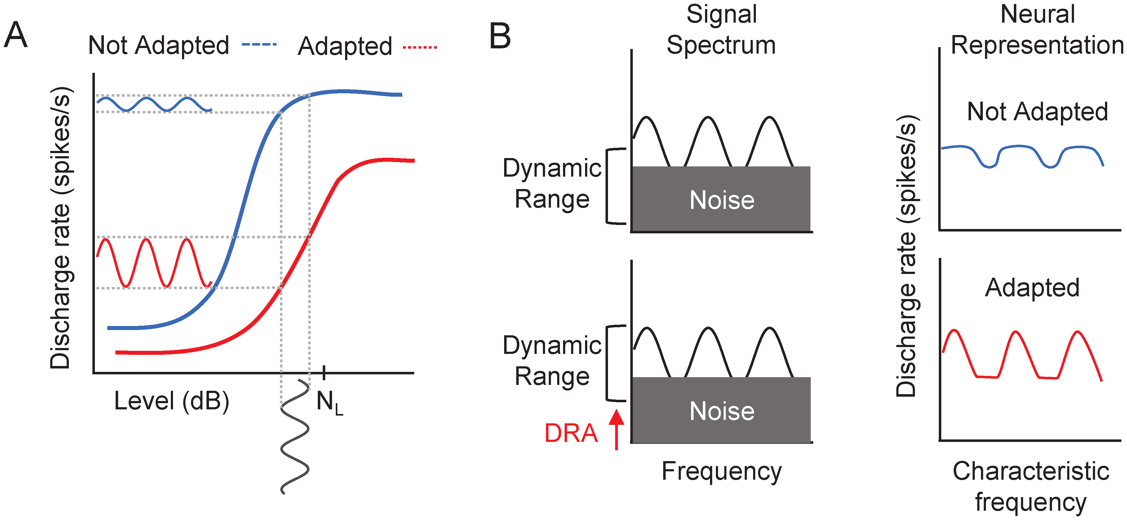
Schematic representation of the effect of neural dynamic range adaptation (DRA) on the encoding of temporal (A) and spectral envelopes (B). (A) The temporal envelope (black solid line) of a signal is poorly encoded when the neuron's response is saturated (blue solid line). However, when the neuron shifts its dynamic range toward the noise level (N_L), the encoding of the temporal envelope improves (red dotted line). Figure adapted from Marrufo-Pérez et al. (2018a). (B) Similarly, the spectral envelope (black solid line) could be poorly encoded in the neural rate profile when auditory neurons are saturated (blue solid line) but could be more faithfully encoded thanks to dynamic range adaptation (red dotted line). Figure adapted from Ainsworth and Meyer (1994).

Speech signals contain TM, SM, and STM. TM pertain to variations in energy over time, while SM manifest as changes in energy over frequency. STM combine SM and TM, thus appear in spectrograms as diagonal energy shifts (Figure 2). Speech recognition depends primarily on the information contained in the low SM (<4 cycles/kHz) and slow TM (<12 Hz) (e.g., Elliott & Theunissen, 2009). The ability of the auditory system to accurately encode the pattern of modulations contained in speech is paramount for successful speech recognition. Indeed, recognition worsens when speech is spectrally (Ainsworth & Millar, 1972; Liu & Eddins, 2008; van Veen & Houtgast, 1985; Zahorian & Jagharghi, 1993) or temporarily degraded (Drullman et al., 1994). [Of course, it is not possible to reduce the temporal information in speech without affecting the spectral information or vice versa (Drullman et al., 1994).]. Therefore, any process that improves the encoding of speech modulations, for example, dynamic range adaptation, could facilitate speech recognition.

Figure 2.

Example spectrograms of the stimuli used in the spectral (first row), temporal (second row), and spectrotemporal modulation detection tasks (third row). The target signal (broadband ripple noise) is shown in yellow. The background noise (white noise) is represented in green, and silence is shown in blue. The left column illustrates the stimuli in the early condition, with a 50ms noise-signal onset delay. The right column illustrates the stimuli in the late condition, with an 800ms noise-signal onset delay. The noise always ended 50ms after the signal offset. For illustration purposes, the modulation phase was equal for all the stimuli. SM=spectral modulation; STM=spectrotemporal modulation; TM=temporal modulation.

It is not yet clear whether adaptation to noise in speech recognition results from an improvement in the encoding of TM, SM, or STM speech cues. Regarding TM, previous studies have shown that for AM signals in noise, AM detection improves when the signal is delayed in the noise (Marrufo-Pérez et al., 2018b) or preceded by a noise precursor (Almishaal et al., 2017; Wojtczak et al., 2019). These results are consistent with an improvement in the encoding of TM related to dynamic range adaptation in auditory neurons (Figure 1). Because of this, one might think that adaptation to noise in speech recognition may be mediated by an enhancement of the speech TM when speech is delayed in the noise. However, as shown in Figure 1, dynamic range adaptation could also enhance the encoding of SM. Indeed, computer model simulations (Ainsworth & Meyer, 1994) show that automatic speech recognition improves as the speech spectral contrast in the AN rate profile improves when AN fibers shift their thresholds toward the noise level. However, unlike for TM, it is yet to be empirically shown that for signals in noise, the sensitivity to SM or STM improves as the signal is delayed in the noise.

One aim of the present study was to experimentally investigate if there is adaptation to noise in the detection of SM and STM. Another aim was to investigate which type of modulation cue may be involved in adaptation to noise in speech recognition. We hypothesized that if adaptation occurs for all three types of modulations (TM, SM, and STM), then adaptation in word recognition might be related to improvements in the encoding of one or more of those three modulation cues. However, if adaptation does not occur for SM or STM, then this would suggest that the modulation cue in question is unlikely involved in adaptation to noise in speech recognition.

Methods

Experimental Design and Hypotheses

We measured noise adaptation in word recognition and modulation detection for the same participants (paired design). Adaptation in modulation detection was measured using spectral, temporal, and spectrotemporal ripple noise. This stimulus was chosen, first, because the sensitivity to spectrotemporal ripples can partly predict speech recognition in noise (Bernstein et al., 2013, 2016; Davies-Venn et al., 2015; Henry et al., 2005; Mehraei et al., 2014; Zaar et al., 2023); and, second, because the use of ripple noise allows measuring noise adaptation in the detection of TM and SM when the two types of modulation occur separately, but also when they occur simultaneously (see below). Therefore, the use of ripple noise allows investigating whether noise adaptation differs depending on the nature of the modulation.

Adaptation in speech recognition was measured using isolated words that were unprocessed (natural) or processed (vocoded) to have poor spectral and temporal fine structure information but preserve temporal envelope cues (Shannon et al., 1995). Adaptation was measured for these two types of words, first, because adaptation is overall greater for vocoded than for natural words (Marrufo-Pérez et al., 2018a; 2020). A second reason is that vocoded-word recognition relies mostly on detecting and processing TM, much less so on SM, and not at all on temporal fine structure (TFS) speech cues (Shannon et al., 1995). Therefore, adaptation in modulation detection may be more relevant for adaptation in the recognition of vocoded than natural words.

Adaptation to noise is usually quantified as the improvement in performance when the target signal is delayed in the noise (reviewed by Marrufo-Pérez & Lopez-Poveda, 2022). The same noise adaptation paradigm was employed across all tasks to facilitate the comparison of the results in the word recognition and modulation detection tasks. Specifically, white noise (1–22050 Hz) at 60 dB SPL was used as the background noise. Noise adaptation was quantified as the difference in performance between an “early” and a “late” condition. In the early condition, the target signal (word or ripple noise) was presented 50 ms after the onset of the noise. In the late condition, the onset of the target signal was delayed 800 ms from the noise onset. In both conditions, the background noise ended 50 ms after the end of the signal (Figure 2).

The experiments were approved by the Ethics Review Board of the University of Salamanca.

Participants

Eighteen adults (five men) with normal hearing (NH) participated in the experiments (mean ± SD age = 26.6 ± 5.6 years). Seventeen of them had audiometric thresholds ≤ 20 dB hearing level (HL) at octave frequencies between 125 and 8000 Hz in the test (left) ear (ANSI, 1996). One participant had an audiometric threshold of 25 dB HL at 8000 Hz. Sixteen participants were native speakers of Spanish, while the other two were native speakers of Portuguese but were proficient in Spanish (their speech recognition and adaptation scores were not outliers according to Tukey's rule). They were not paid for their services. All participants signed an informed consent form to participate in the study.

Test Sessions

The experimental protocol consisted of multiple sessions in which participants performed word recognition and/or STM detection tasks. The first session was devoted to performing the tasks in quiet, which allowed participants to become familiar with the stimuli and tasks. Subsequent sessions were devoted to performing the tasks in noise. In these sessions, the early and late conditions were always measured in pairs but were administered in random order. Participants completed every task three times in three separate blocks. In each block, tasks were administered in random order. The total duration of the experiment was approximately 6 h. Participants took breaks as needed.

Spectrotemporal Modulation Detection Tasks

Stimuli

The target signal was a broadband ripple noise like the one used by Chi et al. (1999). The ripple noise consisted of 92 random-phase tones equally spaced along the logarithmic frequency axis between 140 and 7340 Hz (5.75 octaves).

The ripple profile in the temporal and spectral domains wasdetermined by the following equation:

S (x, t) = A \cdot \sin [2 π (ω t + Ω x) + ϕ],

(1)

where x is the position on the logarithmic frequency axis (in octaves): x = log₂(f/f₀) with f₀ = 140 Hz as the lower edge of the spectrum, and f as the frequency; t the time; A the amplitude of the ripple profile relative to a flat ripple (or modulation depth), with A = 0 corresponding to the unmodulated ripple, and A = 1 corresponding to a fully modulated ripple; ω is defined as the ripple velocity (number of ripple cycles per second) in Hz; Ω the ripple density in cycles/octave (c/o); and ϕ the phase of the profile, which was set to a random value between 0 and 2π radians every time a ripple noise was generated.

The duration of the ripple noise was 200 ms, and its overall level 60 dB SPL. Therefore, the signal-to-noise ratio (SNR) in the noise tasks was 0 dB (note that because the background noise was white and the ripple noise had a downward-sloping spectra, the SNR was, in fact, positive at lower frequencies and negative at higher frequencies). In the SM detection task, Ω was set to 2 c/o, whereas ω was set to 0 Hz (i.e., no TM). In the TM detection task, Ω was set to 0 c/o (i.e., no SM) and ω was set to 10 Hz. In the STM detection task, Ω was set to 2 c/o and ω was set to 10 Hz, which resulted in a downward-moving ripple. Figure 2 shows the spectrograms of the stimuli for each modulation detection task. Low ripple density and velocity were chosen because low SM and slow TM contribute the most to speech intelligibility (Elliott & Theunissen, 2009). Furthermore, SM sensitivity in quiet at the same ripple density of this study (2 c/o) showed a significant correlation with speech intelligibility in noise (Bernstein et al., 2013, 2016; Zaar et al., 2022). The ripple velocity (10 Hz) used here was chosen to guarantee at least two AM cycles over the used stimulus duration (200 ms). This ripple velocity was intermediate to the values used in previous studies [4 Hz in Zaar et al. (2022) and up to 32 Hz in Bernstein et al. (2013)].

In this task, the duration of the background noise was 300 ms in the early condition (50ms signal-noise onset delay, plus 200ms signal duration, plus 50ms noise-signal offset delay) and 1050 ms in the late condition (800 ms + 200 ms + 50 ms).

Procedure

Modulation detection thresholds were measured using a three-alternative forced-choice procedure. Each trial consisted of three observation intervals. The modulated ripple noise was randomly assigned to one of them, and the other two intervals contained the unmodulated ripple noise. The participant had to choose the interval in which the modulated stimulus was presented. Feedback was provided on the correctness of the response. The modulation depth (A) in dB full scale (FS), that is, L_A = 20۰log₁₀(A), was varied adaptively following a “two-down, one-up” rule (i.e., the modulation depth decreased after two correct responses and increased after an incorrect response) that leads to the 70.7% correct response point on the psychometric curve (Levitt, 1971). The initial modulation depth was set to A = 1 (0 dB), that is, the ripple noise was fully modulated. The procedure continued until 12 reversals in modulation depth were recorded. For the first six reversals, the modulation depth changed in 4dB steps; for the remaining reversals, the step was 2 dB. The detection threshold was calculated as the mean modulation depth at the last eight reversals. The threshold for each participant and condition was the mean of three measurements. At the start of each trial, a pure tone (1000 Hz) was presented to alert the participant as to the start of the stimulus presentation.

Control Experiment With Upward-Moving Ripple

While some studies have suggested that upward-moving ripples are more easily detected than downward-moving ripples (Chi et al., 1999; Zaar et al., 2022), other studies suggest that the direction of the ripple has no effect on modulation detection thresholds (Bernstein et al., 2013; Mehraei et al., 2014; Oetjen & Verhey, 2015). Here, a control experiment was performed to investigate if the direction of the ripple could affect the magnitude of adaptation to noise in STM detection. In this control experiment, Ω was set to 2 c/o and ω was set to −10 Hz (notice the negative sign), which resulted in an upward-moving ripple. Otherwise, the stimuli and procedure were as in the main experiment. Thirteen NH adults performed this control experiment, two of whom had completed the main experiment.

Speech Recognition Task

Stimuli

Speech reception thresholds (SRTs) were measured using the corpus of phonetically balanced, Castilian-Spanish disyllabic words of Cárdenas and Marrero (1994). Twenty-five words corresponding to one of the 10 available lists were used to measure each SRT. The same corpus was used to measure SRTs for vocoded words. The vocoder (Shannon et al., 1995) included a high-pass pre-emphasis filter (first-order Butterworth filter with a 3dB cutoff frequency of 1.2 kHz), a bank of 12 sixth-order Butterworth band-pass filters whose 3dB cutoff frequencies followed a modified logarithmic distribution between 100 and 8500 Hz, and envelope extraction via full-wave rectification and low-pass filtering (fourth-order Butterworth low-pass filter with a 3dB cutoff frequency of 400 Hz). The envelope for each frequency channel was used to modulate the amplitude of a sinusoidal carrier at the channel center frequency. The modulated carriers were filtered again through the corresponding band-pass filter, and sample-wise added to obtain the vocoded speech.

Eighteen SRTs were measured for each participant: 2 word types (natural and vocoded) × 3 conditions (quiet, early in noise, and late in noise) × 3 measurements per word type per condition. Because only 10 different word lists were available, it was necessary to repeat eight lists for each participant. Words were presented in random order across conditions to minimize the chance that participants remembered them.

Procedure

The SRT in noise was defined as the SNR (in dB) at 50% recognition (Levitt, 1971). It was measured by adaptively varying the speech level using a “one-down, one-up” rule. The task started with an initial SNR of 20 dB. The speech level was varied in 4dB steps for the first 14 words, and in 2dB steps for the last 11 words. The SRT was calculated as the mean SNR for the last 17 words. At the beginning of each trial, a 1000Hz pure tone was presented as a warning. Participants were not given feedback on the correctness of their responses. The SRT reported for each participant is the mean of three SRT estimates.

Equipment

During the experiments, participants were seated in a double-walled sound-attenuating chamber. Stimuli were digitally stored (word recognition) or generated (modulation detection) and presented using custom-made MATLAB software (R2017b, The MathWorks). Stimuli were played via an RME Fireface UCX soundcard at a sampling rate of 44100 Hz with a 24-bit resolution. Stimuli were presented monaurally to the participants’ left ear through Sennheiser HD-580 headphones. The equipment was calibrated by placing the headphones on a KEMAR (Knowles Electronics) equipped with a Zwislocki DB-100 coupler (Knowles Electronics) connected to a sound level meter (Brüel Kjaer, mod. 2238). Calibration was performed at 1000 Hz, and the obtained sensitivity was used for all other frequencies.

Statistical Analyses

Statistical analyses were performed using the rstatix (Kassambara, 2021) package in R (version 4.1.0). Paired Student's t tests with Bonferroni correction for multiple comparisons were used for pairwise comparisons of thresholds in quiet. Since SRTs were expected to be worse for vocoded than for natural words (Marrufo-Pérez et al., 2018a; 2020), one-tailed t tests were used to compare SRTs for natural and vocoded words. Otherwise, t tests were two-tailed.

To assess the statistical significance of noise adaptation in the different tasks, a two-way repeated measures analysis of variance (RMANOVA) was performed, having the type of task (SM detection, TM detection, STM detection, natural word recognition, and vocoded word recognition) and the noise-signal onset delay (early and late) as factors. When the sphericity condition was not met, the Greenhouse-Geisser correction was applied. To test for the effect of ripple direction, a mixed two-way analysis of variance (ANOVA) was performed, including the ripple direction (downward, upward) as a between-subjects factor and the temporal position (early, late) as a repeated measures factor.

Paired Student's t tests with Bonferroni corrections for multiple comparisons were applied for post hoc pairwise comparisons. The test to compare the magnitude of adaptation between natural and vocoded words was one-tailed, as we expected adaptation to be greater for vocoded words (Marrufo-Pérez et al., 2018a; 2020). All other post hoc tests were two-tailed.

Results

Thresholds in Quiet

Figure 3A shows the SRTs for natural and vocoded words in quiet. The mean SRTs were significantly lower (better) for natural (mean ± SD = 22.7 ± 2.9 dB SPL) than for vocoded words (27.1 ± 4.0 dB SPL) (paired Student's t test: t₍₁₇₎= −8.08, p < .001).

Figure 3.

Violin plots showing the distribution of speech reception thresholds (SRTs) for natural and vocoded words (A) and detection thresholds for spectral (SM), temporal (TM), and spectrotemporal modulations (STM) (B) in quiet. Each violin plot shows the distribution of thresholds (in a distinct color for each stimulus) as well as the individual data (empty circles) and the mean (filled black diamonds). * p ≤ .05; ** p ≤ .01; *** p ≤ .001; ns = not significant.

Figure 3B shows modulation detection thresholds in quiet. The mean TM detection threshold (−10.8 ± 3.7 dB) differed significantly from both the mean SM detection threshold (−13.6 ± 3.6 dB) (paired Student's t test: t₍₁₇₎= −3.38, p = .012) and STM detection threshold (−14.5 ± 3.3 dB) (paired Student's t test: t₍₁₇₎= −4.25, p = .002). However, the mean SM and STM detection thresholds in quiet were not significantly different from each other (paired Student's t test: t₍₁₇₎= 1.11, p = .852).

Adaptation to Noise

Figure 4A shows the SRTs in the early and late conditions for natural and vocoded words, while Figure 4B shows thresholds in the early and late conditions for SM, TM, and STM detection. A two-way RMANOVA with temporal position and task as factors revealed that mean thresholds were overall lower (better) in the late than in the early condition (F_(1,17) = 91.13, p < .001) (i.e., a significant effect of adaptation to noise). In addition, the interaction between task and temporal position was also significant (F_(4,68) = 7.20, p < .001), which indicated that the magnitude of adaptation to noise was different across tasks. Post hoc comparisons showed that the SRT improvement in the late condition was not significant for natural words (paired Student's t test: t₍₁₇₎ = 1.90, p = .19), but was significant for vocoded words (paired Student's t test: t₍₁₇₎ = 5.44, p < .001). Adaptation to noise was statistically significant for SM (paired Student's t test: t₍₁₇₎= 5.19, p < .001) and TM (paired Student's t test: t₍₁₇₎ = 4.37, p = .002) detection, but not for STM detection (paired Student's t test: t₍₁₇₎=−0.19, p = 1.0).

Figure 4.

Violin plots showing the distribution of speech reception thresholds (SRTs) for natural and vocoded words (A) and detection thresholds for spectral (SM), temporal (TM), and spectrotemporal modulations (STM) (B) in the early (green) and late (orange) condition. Each violin plot shows the distribution of thresholds as well as the individual data (empty circles) and the mean (filled black diamonds). ** p ≤ .01; *** p ≤ .001; ns = not significant.

Figure 5 shows the magnitude of adaptation to noise in the word recognition tasks (a) and modulation detection tasks (b). Mean adaptation was significantly less for natural (0.59 ± 1.3 dB) than for vocoded words (2.1 ± 1.6 dB) (paired Student's t test: t₍₁₇₎=−3.50, p = .004). This is consistent with previous studies that also found greater adaptation to noise in vocoded word recognition than in natural word recognition (Marrufo-Pérez et al., 2018a, 2020). Regarding modulation detection, noise adaptation in SM (2.1 ± 1.7 dB) and TM (2.2 ± 2.1 dB) detection was significantly different from adaptation in STM detection (−0.04 ± 0.9 dB) (paired Student's t test: t₍₁₇₎ = 4.56, p = .001; paired Student's t test: t₍₁₇₎ = 4.15, p = .003, respectively). The difference between adaptation to noise in SM and TM detection was not significant (paired Student's t test: t₍₁₇₎=−0.21, p = 1.0).

Figure 5.

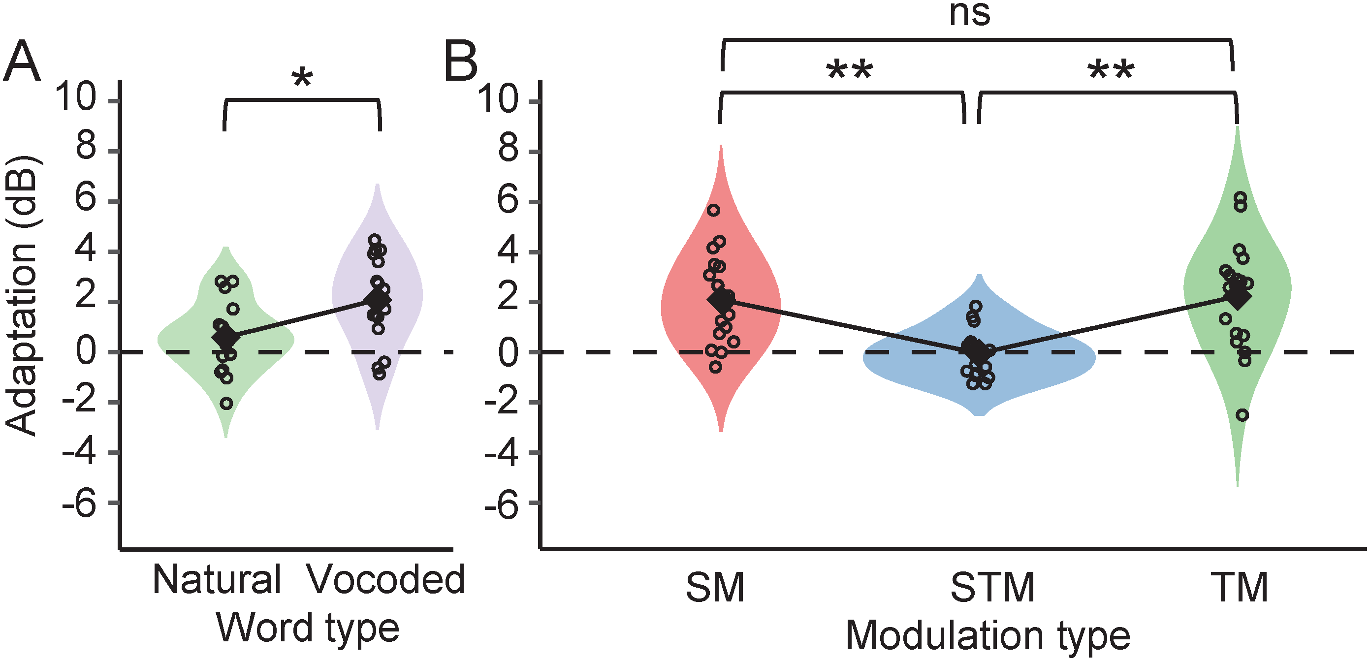
Violin plots showing the distribution of the values of adaptation in natural and vocoded word recognition (A) and in spectral (SM), temporal (TM), and spectrotemporal modulation (STM) detection (B). Each violin plot shows the distribution of the values (in a distinct color for each stimulus) as well as the individual data (empty circles) and the mean (filled black diamonds). * p ≤ .05; ** p ≤ .01.

Control Experiment With Upward-Moving Ripple

Figure 6A shows the modulation detection thresholds in the early and late conditions for the upward-moving STM ripple noise. Corresponding thresholds for the downward-moving ripples were shown in Figure 4B (STM dataset). A mixed, two-way ANOVA with temporal position as repeated-measures factor and direction (downward or upward) as intersubject factor revealed nonsignificant effects of temporal position (F_(1,29) = 1.51, p = .229) or ripple direction (F_(1,29) = 1.70, p = .203) as well as a nonsignificant interaction of these two factors (F_(1,29) = 1, p = .327). Adaptation measured with upward-moving ripple (−0.4 ± 1.1 dB) was not statistically significant (paired Student's t test: t₍₁₇₎=−1.32, p = .894) and did not differ from the one measured with downward-moving ripple (Student's t test: t₍₂₉₎ = 1, p = .327; Figure 6B). In addition, modulation detection thresholds in quiet (data not shown) did not differ for downward-moving and upward-moving ripples (Student's t test: t₍₂₉₎=−0.253, p = .802), consistent with results reported in previous studies (Bernstein et al., 2013; Mehraei et al., 2014; Oetjen & Verhey, 2015). Thus, we conclude that the lack of an improvement in STM detection when delaying the signal from the noise onset does not depend on the direction of the modulation.

Figure 6.

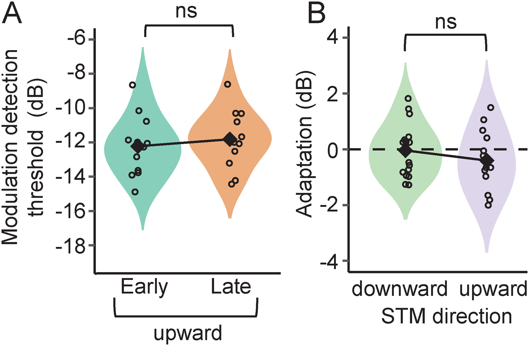
(A) Violin plots showing the distribution of detection thresholds for upward spectrotemporal modulations (STM). (B) The distribution of the values of adaptation in downward (replotted from Figure 5B, STM dataset) and upward STM detection. Each violin plot shows the distribution of the values as well as the individual data (empty circles) and the average (filled black diamonds). ns = not significant.

Discussion

One aim of the present study was to investigate if there is adaptation to noise in the detection of TM, SM, and STM using ripple noise. We hypothesized that if neural dynamic range adaptation participates in adaptation to noise, it should improve the neural representation, thus the detection of SM as well as TM (Figure 1). We found that noise adaptation occurs in the detection of TM and SM, but not in the detection of combined STM(Figures 4 and 5).

Another aim was to investigate which type of modulation may be involved in adaptation to noise in word recognition. We hypothesized that word-in-noise recognition may be better in the late than in the early condition because dynamic range adaptation improves the neural encoding of speech (SM, TM, and/or STM) modulation cues in the late condition. If this were the case, adaptation to noise in modulation detection should occur for all three types of modulations. Consistent with previous studies, we found statistically significant adaptation in the recognition of vocoded words, but not in the recognition of natural words (Figure 5A). However, in contrast to expectations, for the same listeners, adaptation to noise occurred in SM and TM detection but not in STM detection (Figure 5B). This suggests that STM detection cues may not be involved in adaptation to noise in speech recognition.

Adaptation to Noise in Modulation Detection

As far as we know, this is the first study that empirically demonstrates an improvement in SM detection as the SM signal is delayed from the noise onset. Our findings, however, are consistent with the computer model simulations of Ainsworth and Meyer (1994). They showed that the speech spectrum was better encoded in the AN rate profile when speech was presented in continuous than in gated background noise. In their model, the improvement was the result of including a shift in the threshold and dynamic range of AN fibers toward the noise level in the continuous background noise condition.

Regarding TM detection, the mechanism for detecting temporal ripples superimposed on a noise could be the same as that used for detecting sinusoidal AM superimposed on a tone. Unfortunately, a direct comparison between noise adaptation in TM detection as measured here with the adaptation found in previous AM detection studies is not straightforward because the amount of adaptation depends on the modulation rate (Almishaal et al., 2017; Sheft & Yost, 1990; Viemeister, 1979), the sound level (Almishaal et al., 2017; although see Wojtczak et al., 2019), the laterality and type of noise (Marrufo-Pérez et al., 2018b; Wojtczak et al., 2019), the stimulus type [pure tone (Marrufo-Pérez et al., 2018b; Wojtczak et al., 2019) vs. noise (Almishaal et al., 2017; Sheft & Yost, 1990; Viemeister, 1979)], and the testing paradigm [use of precursors (Almishaal et al., 2017; Wojtczak et al., 2019) vs. delay from noise onset (Marrufo-Pérez et al., 2018b)]. For a review of adaptation to noise in AM detection, see Marrufo-Pérez and Lopez-Poveda (2022).

The improvement in sensitivity to SM and TM as they are delayed from the noise onset could be explained by a noise-induced shift of the neural dynamic range (as shown in Figure 1). But why would dynamic range adaptation not enhance the sensitivity to combined SM and TM? The reason is unknown, but Figure 7 illustrates a hypothetical explanation based on dynamic range adaptation in the AN (Ainsworth & Meyer, 1994; Marrufo-Pérez et al., 2018b). The figure schematically illustrates the AN representation of SM, TM, and STM stimuli presented early and late in noise. The shown rate-level functions are for a hypothetical AN fiber with (dotted lines) and without (continuous lines) a noise-induced shift of the threshold and dynamic range towards the noise level (N_L). As the stimuli are “passed” through rate-level functions for apopulation of AN fibers, dynamic range adaptation would enhance the three kinds of modulations as illustrated by the greater contrast between peaks and valleys in the AN representation in the late than in the early condition. There exist central auditory neurons that integrate neural responses across time (e.g., multipolar neurons in the cochlear nucleus, Blackburn & Sachs, 1990; or neurons in the central nucleus of the inferior colliculus, Rodríguez et al., 2010) or characteristic frequency (CF) (e.g., octopus cells in the cochlear nucleus, Oertel et al., 2000; or neurons in the central nucleus of the inferior colliculus, Rodríguez et al., 2010) presumably to provide stable representations of the stimulus spectrum and envelope. If modulation sensitivity depends on integrating neural population responses, a greater sensitivity to SM is predicted in the late condition when the AN responses are integrated across time. Likewise, a greater sensitivity to TM in the late condition is predicted when the AN responses are integrated across CFs. However, if STMs are detected by the same mechanism as SMs (i.e., by resolving spectral peaks and valleys) (Bernstein et al., 2013, 2016; Davies-Venn et al., 2015; Eddins & Bero, 2007; Isarangura et al., 2019; Narne et al., 2016, 2018; Summers & Leek, 1994) little or no change in sensitivity to STM is predicted in the late condition. The same would happen if STMs were detected by using the integrated AN response across CFs.

Figure 7.

Hypothetical explanation for the absence of adaptation to noise in the detection of spectrotemporal modulation. (A) Schematic illustration of the effect of a shift in the dynamic range of AN fibers on the AN representation of spectral (first row), temporal (second row) and spectrotemporal modulations (third row). Rate-level functions are shown with (dotted lines) and without (continuous lines) a hypothetical noise-induced shift of their threshold and dynamic range. The AN representation of the three modulations is enhanced (higher contrast) in the late condition than in the early condition (lower contrast) because of this shift in the dynamic range of the fibers. (B) Schematic representation of each modulation type when AN spikes are integrated across time (rate profile, first column) and across CFs (second column). After integration, spectral, and temporal envelopes are better represented in the late condition for spectral and temporal modulations but not for spectrotemporal modulations (see the main text for details). AN=auditory nerve; CF=characteristic frequency.

The detection of SM and STM may not always depend on the ability to resolve the spectral peaks and valleys of the modulation. Several cues such as local spectral loudness, a different spectral centroid between the reference and target stimuli, and/or differences at the spectral boundaries of the reference and target stimuli (Aronoff & Landsberger, 2013; Azadpour & McKay, 2012) can influence the discrimination/detection of SM. In addition, STM detection could be mediated by an AM cue at the output of the auditory filters at the lower and upper spectral limits of the ripple noise (Narne et al., 2016). In the present study, local loudness cues, or differences in the spectral centroid or at the spectral boundaries were unreliable cues for SM detection because a random phase was applied each time the ripple noise was generated (Aronoff & Landsberger, 2013). Likewise, the AM cue at the output of the auditory filters at the spectral edges of the ripple noise would be masked by the noise. Hence, here, STM detection probably relied on resolving spectral peaks, that is, on the same mechanism proposed to detect SM. In fact, because the background noise was white and the ripple noise had a downward-sloping spectra, SM and STM detection probably involved resolving the spectral peaks in the low-frequency region, where the SNR was higher.

Of course, the hypothetical mechanism illustrated in Figure 7 is an oversimplification and almost certainly inaccurate. For example, as it stands, it would predict worse thresholds for STM detection than for SM or TM detection because STM would be smeared when integrating neural responses across time and/or CF. This prediction is not consistent with the experimental data, as STM detection thresholds were close to SM detection thresholds and better than TM detection thresholds. However, Figure 7 represents a hypothetical extreme case where the spectral and temporal integration windows span the entire stimulus. It is likely that the auditory system integrates neural responses using smaller windows, thus the loss of STM information is probably less than suggested by Figure 7. In addition, Bernstein et al. (2013) found that the sensitivity to frequency modulation (FM) at 2 Hz applied to a 500Hz pure-tone carrier was a significant predictor of STM sensitivity. Assuming that FM sensitivity at low modulation rates is encoded in the timing of neural spikes via phase locking (e.g., Moore & Sek, 1996; but see Whiteford et al., 2020), the findings of Bernstein et al. (2013) suggest that STM sensitivity might depend on the ability to use TFS cues. This possibility is disregarded in Figure 7.

Other phenomena besides neural dynamic range adaptation may have contributed to the current results. For example, thresholds might have been better in the late than in the early condition because the background noise functioned as warning and drew the listener's attention to the task. However, we tried to minimize this effect by presenting a pure tone cue at the beginning of each trial. Furthermore, if this attentional driven improvement in sensitivity had occurred, it would have affected performance equally in all modulation detection tasks. The fact that detectability in the late condition improved for SM and TM detection but not for STM detection undermines this mechanism as an explanation for adaptation to noise. Modulation masking could have also contributed to the current results, that is, the onset of background noise could be interpreted as a TM (Gallun & Hafter, 2006). The onset of the background noise was closer in time to the signal in the early than in the late condition. This could have caused some modulation masking in the early condition, making it seem that modulation sensitivity was worse in the early than in the late condition. However, while this phenomenon could have affected TM detection, it is unclear how it could have affected SM or STM detection.

Less Noise Adaption for Natural Than for Vocoded Words

Like previous studies (e.g., Marrufo-Pérez et al., 2018a, 2020), we have found greater adaptation to noise in vocoded than in natural word recognition. Two explanations have been proposed elsewhere for this result. The first one (proposed by Marrufo-Pérez et al., 2018a, 2020) relates to a ceiling effect: because SRTs tend to be better (lower) for natural than vocoded words, there is less room for SRT improvement for natural than vocoded words. The second explanation (proposed by Marrufo-Pérez et al., 2020) is that improved envelope cues may be less effective when word recognition relies in part on TFS encoding, as may be the case for natural words (Hopkins & Moore, 2009).

Intriguingly, the present data show that explanation #1 does not hold for modulation detection tasks as thresholds in the early condition were nearly identical for SM and STM detection, and adaptation was statistically significant only in SM detection. Moreover, although thresholds were worse for TM than SM detection in the early condition, adaptation was similar for the two tasks. Explanation #2, however, would be supported by the present data if TFS information played a role in STM detection (Bernstein et al., 2013), as we found no adaptation to noise in STM detection or in the recognition of natural words.

Relationship Between Adaptation in Modulation Detection and Speech Recognition

Dynamic range adaptation can improve the neural encoding of SM and TM (Figure 1). Both SM and TM are important for speech recognition. Therefore, if dynamic range adaptation is involved in adaptation to noise, one would expect adaptation in modulation detection to occur for the same listeners who show adaptation in speech recognition. We found that noise adaptation occurs for SM and TM detection as well as for vocoded word recognition. This indicates that noise adaptation in (vocoded) word recognition may be mediated by improvements in the neural encoding of sustained SM and/or TM speech cues. However, adaptation did not occur in STM detection (Figure 5). This indicates that it is unlikely that adaptation to noise in (vocoded) word recognition be mediated by improvements in the neural encoding of STM speech cues.

Limitations

Several limitations must be noted. First, different methods were employed to assess word recognition and modulation detection. For example, the SNR was fixed at 0 dB in the modulation detection task while it varied in the word recognition task to measure the individual SRT (the group mean SRT was about −10 dB).

Second, modulation detection was assessed for only one specific TM frequency (10 Hz) and one SM density (2 cpo). Perhaps, adaptation to noise in STM detection might occur for other combinations of TM and SM.

Third, the present data and design were insufficient to elucidate which of the two modulation cues (SM or TM) for which adaptation occurred, if any, is more prominently involved in adaptation in (vocoded) word recognition. This could be investigated, for example, by quantifying the correlation between adaptation in modulation detection and word recognition. Based on the present data, adaptation in vocoded word recognition was not correlated with adaptation in SM or TM detection (not shown). However, a larger participant sample or a sample with more variable adaptation scores would be needed to address this question using correlational analyses with enough statistical power.

Fourth, the present modulation detection tasks assess a listener's sensitivity to sustained modulations. However, transient information, such as vowel formant transitions, is essential for speech perception. For example, Varnet et al. (2013) showed that listeners use mainly the end of the second formant (F2) in the first vowel and the onset of F2 in the second vowel as cues to discriminate between /aba/ and /ada/. Liberman et al. (1954) also showed that F2 transitions are key for distinguishing between these two phonemes. In other words, the recognition of disyllabic words in noise could depend on detecting a word's transient features as well as on detecting their (long-term) temporal or spectral envelopes. Therefore, adaptation to noise in word recognition may also be related to improvements in the neural encoding of speech transients, something that was not explored here.

Conclusions

For signals in noise, the sensitivity to SM and TM but not to STM improves as the signal is delayed 800 ms from the noise onset. In other words, adaptation to noise occurs in the detection of SM and TM but not in the detection of combined SM and TM.

The recognition of words in noise can improve as words are delayed 800 ms in the noise. The improvement was statistically significant for vocoded but not for natural words.

Therefore, adaptation to noise in word recognition may be mediated by improvements in the neural encoding of sustained SM or TM, but it is unlikely mediated by improvements in the encoding of combined STM.

Footnotes

Data Availability

Data are available from the authors upon request.

Acknowledgments

We thank Milagros J. Fumero and Wendy Vilchez Ugalde for help with data collection. We also thank the editors.

Declaration of Conflicting Interests

The authors report no conflicting interests.

Funding

The authors disclosed receipt of the following financial support for the research, authorship, and/or publication of this article: This work was supported by the Banco Santander, Ministerio de Ciencia e Innovación, European Regional Development Fund, Ministerio de Universidades, Universidad de Salamanca, (grant number PID2019-108985GB-I00). DLR was hired on a doctoral contract of the University of Salamanca and Banco Santander. MIMP was hired by a Margarita Salas research contract of the Spanish Ministry of Universities.

ORCID iDs

David López-Ramos

Luis E. López-Bascuas

Enrique A. Lopez-Poveda

References

Ainsworth

W. A.

Meyer

G. F.

(1994). Recognition of plosive syllables in noise: Comparison of an auditory model with human performance. The Journal of the Acoustical Society of America, 96(2), 687–694. https://doi.org/10.1121/1.410306

Ainsworth

W. A.

Millar

J. B.

(1972). The effect of relative formant amplitude on the perceived identity of synthetic vowels. Language and Speech, 15(4), 328–341. https://doi.org/10.1177/002383097201500403

Almishaal

Bidelman

G. M.

Jennings

S. G.

(2017). Notched-noise precursors improve detection of low-frequency amplitude modulation. The Journal of the Acoustical Society of America, 141(1), 324–333. https://doi.org/10.1121/1.4973912

American National Standars Institute (1996). S3.6 Specification for audiometers. American National Standards Institute.

Aronoff

J. M.

Landsberger

D. M.

(2013). The development of a modified spectral ripple test. The Journal of the Acoustical Society of America, 134(2), EL217–EL222. https://doi.org/10.1121/1.4813802

Azadpour

McKay

C. M.

(2012). A psychophysical method for measuring spatial resolution in cochlear implants. Journal of the Association for Research in Otolaryngology, 13(1), 145–157. https://doi.org/10.1007/s10162-011-0294-z

Bacon

S. P.

Takahashi

G. A.

(1992). Overshoot in normal-hearing and hearing-impaired subjects. The Journal of the Acoustical Society of America, 91(5), 2865–2871. https://doi.org/10.1121/1.402967

Ben-David

B. M.

Tse

V. Y. Y.

Schneider

B. A.

(2012). Does it take older adults longer than younger adults to perceptually segregate a speech target from a background masker? Hearing Research, 290(1-2), 55–63. https://doi.org/10.1016/j.heares.2012.04.022

Bernstein

J. G. W.

Danielsson

Hällgren

Stenfelt

Rönnberg

Lunner

(2016). Spectrotemporal modulation sensitivity as a predictor of speech-reception performance in noise with hearing aids. Trends in Hearing, 20, 1–17. https://doi.org/10.1177/2331216516670387

10.

Bernstein

J. G. W.

Mehraei

Shamma

Gallun

F. J.

Theodoroff

S. M.

Leek

M. R.

(2013). Spectrotemporal modulation sensitivity as a predictor of speech intelligibility for hearing-impaired listeners. Journal of the American Academy of Audiology, 24(4), 293–306. https://doi.org/10.3766/jaaa.24.4.5

11.

Blackburn

C. C.

Sachs

M. B.

(1990). The representations of the steady-state vowel sound /ε/ in the discharge patterns of cat anteroventral cochlear nucleus neurons. Journal of Neurophysiology, 63(5), 1191–1212. https://doi.org/10.1152/jn.1990.63.5.1191

12.

Cárdenas

M. R.

Marrero

(1994). Cuaderno de logoaudiometría. Universidad Nacional de Educación a Distancia.

13.

Cervera

Ainsworth

W. A.

(2005). Effects of preceding noise on the perception of voiced plosives. Acta Acustica United with Acustica, 91(1), 132–144.

14.

Cervera

Gonzalez-Alvarez

(2007). Temporal effects of preceding band-pass and band-stop noise on the recognition of voiced stops. Acta Acustica United with Acustica, 93(6), 1036–1045.

15.

Chi

Gao

Guyton

M. C.

Shamma

(1999). Spectro-temporal modulation transfer functions and speech intelligibility. The Journal of the Acoustical Society of America, 106(5), 2719–2732. https://doi.org/10.1121/1.428100

16.

Costalupes

J. A.

Young

E. D.

Gibson

D. J.

(1984). Effects of continuous noise backgrounds on rate response of auditory nerve fibers in cat. Journal of Neurophysiology, 51(6), 1326–1344. https://doi.org/10.1152/jn.1984.51.6.1326

17.

Davies-Venn

Nelson

Souza

(2015). Comparing auditory filter bandwidths, spectral ripple modulation detection, spectral ripple discrimination, and speech recognition: Normal and impaired hearing. The Journal of the Acoustical Society of America, 138(1), 492–503. https://doi.org/10.1121/1.4922700

18.

Dean

Harper

N. S.

McAlpine

(2005). Neural population coding of sound level adapts to stimulus statistics. Nature Neuroscience, 8(12), 1684–1689. https://doi.org/10.1038/nn1541

19.

Dean

Robinson

B. L.

Harper

N. S.

McAlpine

(2008). Rapid neural adaptation to sound level statistics. Journal of Neuroscience, 28(25), 6430–6438. https://doi.org/10.1523/JNEUROSCI.0470-08.2008

20.

Drullman

Festen

J. M.

Plomp

(1994). Effect of reducing slow temporal modulations on speech reception. The Journal of the Acoustical Society of America, 95(5), 2670–2680. https://doi.org/10.1121/1.409836

21.

Eddins

D. A.

Bero

E. M.

(2007). Spectral modulation detection as a function of modulation frequency, carrier bandwidth, and carrier frequency region. The Journal of the Acoustical Society of America, 121(1), 363–372. https://doi.org/10.1121/1.2382347

22.

Elliot

L. L.

(1965). Changes in the simultaneous masked threshold of brief tones. The Journal of the Acoustical Society of America, 38(5), 738–746. https://doi.org/10.1121/1.1909798

23.

Elliott

T. M.

Theunissen

F. E.

(2009). The modulation transfer function for speech intelligibility. PLoS Computational Biology, 5(3), e1000302. https://doi.org/10.1371/journal.pcbi.1000302

24.

Evans

E. F.

(1975). Auditory frequency selectivity and the cochlear nerve. In Zwicker

Terhard

(Eds.), Facts and models of hearing (pp. 118–132). Springer-Verlag.

25.

Gallun

F. J.

Hafter

E. R.

(2006). Amplitude modulation sensitivity as a mechanism for increment detection. The Journal of the Acoustical Society of America, 119(6), 3919–3930. https://doi.org/10.1121/1.2200136

26.

Gibson

D. J.

Young

E. D.

Costalupes

J. A.

(1985). Similarity of dynamic range adjustment in auditory nerve and cochlear nuclei. Journal of Neurophysiology, 53(4), 940–958. https://doi.org/10.1152/jn.1985.53.4.940

27.

Grange

Zhang

Culling

(2022). The role of efferent reflexes in the efficient encoding of speech by the auditory nerve. The Journal of Neuroscience, 42(36), 6907–6916. https://doi.org/10.1523/JNEUROSCI.2220-21.2022

28.

Henry

B. A.

Turner

C. W.

Behrens

(2005). Spectral peak resolution and speech recognition in quiet: Normal hearing, hearing impaired, and cochlear implant listeners. The Journal of the Acoustical Society of America, 118(2), 1111–1121. https://doi.org/10.1121/1.1944567

29.

Hopkins

Moore

B. C. J.

(2009). The contribution of temporal fine structure to the intelligibility of speech in steady and modulated noise. The Journal of the Acoustical Society of America, 125(1), 442–446. https://doi.org/10.1121/1.3037233

30.

Isarangura

Eddins

A. C.

Ozmeral

E. J.

Eddins

D. A.

(2019). The effects of duration and level on spectral modulation perception. Journal of Speech, Language, and Hearing Research, 62(10), 3876–3886. https://doi.org/10.1044/2019_JSLHR-H-18-0449

31.

Jennings

S. G.

Heinz

M. G.

Strickland

E. A.

(2011). Evaluating adaptation and olivocochlear efferent feedback as potential explanations of psychophysical overshoot. Journal of the Association for Research in Otolaryngology, 12(3), 345–360. https://doi.org/10.1007/s10162-011-0256-5

32.

Kassambara

(2021). rstatix: Pipe-Friendly Framework for Basic Statistical Tests. R package version 0.7.0. https://CRAN.R-project.org/package=rstatix.

33.

Levitt

(1971). Transformed up-down methods in psychoacoustics. The Journal of the Acoustical Society of America, 49(2B), 467–477. https://doi.org/10.1121/1.1912375

34.

Liberman

A. M.

Delattre

P. C.

Cooper

F. S.

Gerstman

L. J.

(1954). The role of consonant-vowel transitions in the perception of the stop and nasal consonants. Psychological Monographs: General and Applied, 68(8), 1–13. https://doi.org/10.1037/h0093673

35.

Liu

Eddins

D. A.

(2008). Effects of spectral modulation filtering on vowel identification. The Journal of the Acoustical Society of America, 124(3), 1704–1715. https://doi.org/10.1121/1.2956468

36.

Marrufo-Pérez

M. I.

Eustaquio-Martín

López-Bascuas

L. E.

Lopez-Poveda

E. A.

(2018b). Temporal effects on monaural amplitude-modulation sensitivity in ipsilateral, contralateral and bilateral noise. Journal of the Association for Research in Otolaryngology, 19(2), 147–161. https://doi.org/10.1007/s10162-018-0656-x

37.

Marrufo-Pérez

M. I.

Eustaquio-Martín

Lopez-Poveda

E. A.

(2018a). Adaptation to noise in human speech recognition unrelated to the medial olivocochlear reflex. The Journal of Neuroscience, 38(17), 4138–4145. https://doi.org/10.1523/JNEUROSCI.0024-18.2018

38.

Marrufo-Pérez

M. I.

Lopez-Poveda

E. A.

(2022). Adaptation to noise in normal and impaired hearing. The Journal of the Acoustical Society of America, 151(3), 1741–1753. https://doi.org/10.1121/10.0009802

39.

Marrufo-Pérez

M. I.

Sturla-Carreto

D. d. P.

Eustaquio-Martín

Lopez-Poveda

E. A.

(2020). Adaptation to noise in human speech recognition depends on noise-level statistics and fast dynamic-range compression. The Journal of Neuroscience, 40(34), 6613–6623. https://doi.org/10.1523/JNEUROSCI.0469-20.2020

40.

Mehraei

Gallun

F. J.

Leek

M. R.

Bernstein

J. G. W.

(2014). Spectrotemporal modulation sensitivity for hearing-impaired listeners: Dependence on carrier center frequency and the relationship to speech intelligibility. The Journal of the Acoustical Society of America, 136(1), 301–316. https://doi.org/10.1121/1.4881918

41.

Moore

B. C. J.

Sek

(1996). Detection of frequency modulation at low modulatino rates: Evidence for a mechanism based on phase locking. The Journal of the Acoustical Society of America, 100(4), 2320–2331. https://doi.org/10.1121/1.417941

42.

Narne

V. K.

Prabhu

Van Dun

Moore

B. C. J.

(2018). Ripple glide direction discrimination and its relationship to frequency selectivity estimated using notched noise. Acta Acustica United with Acustica, 104(6), 1063–1074. https://doi.org/10.3813/AAA.919272

43.

Narne

V. K.

Sharma

Van Dun

Bansal

Prabhu

Moore

B. C. J.

(2016). Effects of spectral smearing on performance of the spectral ripple and spectro-temporal ripple tests. The Journal of the Acoustical Society of America, 140(6), 4298–4306. https://doi.org/10.1121/1.4971419

44.

Oertel

Bal

Gardner

S. M.

Smith

P. H.

Joris

P. X.

(2000). Detection of synchrony in the activity of auditory nerve fibers by octopus cells of the mammalian cochlear nucleus. Proceedings of the National Academy of Sciences of the United States of America, 97(22), 11773–11779. https://doi.org/10.1073/pnas.97.22.11773

45.

Oetjen

Verhey

J. L.

(2015). Spectro-temporal modulation masking patterns reveal frequency selectivity. The Journal of the Acoustical Society of America, 137(2), 714–723. https://doi.org/10.1121/1.4906171

46.

Phillips

D. P.

Hall

S. E.

(1986). Spike-rate intensity functions of cat cortical neurons studied continuous noise usually caused a steepening of the slope of the tone intensity. The Journal of the Acoustical Society of America, 80(1), 177–187. https://doi.org/10.1121/1.394178

47.

Rees

Palmer

A. R.

(1989). Neuronal responses to amplitude-modulated and pure-tone stimuli in the Guinea pig inferior colliculus, and their modification by broadband noise. The Journal of the Acoustical Society of America, 85(5), 1978–1994. https://doi.org/10.1121/1.397851

48.

Rodríguez

F. A.

Read

H. L.

Escabi

M. A.

(2010). Spectral and temporal modulation tradeoff in the Inferior colliculus. Journal of Neurophysiology, 103(2), 887–903. https://doi.org/10.1152/jn.00813.2009

49.

Shannon

R. V.

Zeng

Kamath

Wygonski

Ekelid

(1995). Speech recognition with primarily temporal cues. Science, 270(5234), 303–304. http://www.jstor.org/stable/2888543. https://doi.org/10.1126/science.270.5234.303

50.

Sheft

Yost

W. A.

(1990). Temporal integration in amplitude modulation detection. The Journal of the Acoustical Society of America, 88(2), 796–805. https://doi.org/10.1121/1.399729

51.

Summers

Leek

M. R.

(1994). The internal representation of spectral contrast in hearing-impaired listeners. Journal of the Acoustical Society of America, 95(6), 3518–3528. https://doi.org/10.1121/1.409969

52.

van Veen

T. M.

Houtgast

(1985). Spectral sharpness and vowel dissimilarity. The Journal of the Acoustical Society of America, 77(2), 628–634. https://doi.org/10.1121/1.391880

53.

Varnet

Knoblauch

Meunier

Hoen

(2013). Using auditory classification images for the identification of fine acoustic cues used in speech perception. Frontiers in Human Neuroscience, 7(DEC), 1–12. https://doi.org/10.3389/fnhum.2013.00865

54.

Viemeister

N. F.

(1979). Temporal modulation transfer functions based upon modulation thresholds. Journal of the Acoustical Society of America, 66(5), 1364–1380. https://doi.org/10.1121/1.383531

55.

Watkins

P. V.

Barbour

D. L.

(2008). Specialized neuronal adaptation for preserving input sensitivity. Nature Neuroscience, 11(11), 1259–1261. https://doi.org/10.1038/nn.2201

56.

Watkins

P. V.

Barbour

D. L.

(2011). Level-tuned neurons in primary auditory cortex adapt differently to loud versus soft sounds. Cerebral Cortex, 21(1), 178–190. https://doi.org/10.1093/cercor/bhq079

57.

Wen

Wang

G. I.

Dean

Delgutte

(2009). Dynamic range adaptation to sound level statistics in the auditory nerve. The Journal of Neuroscience, 29(44), 13797–13808. https://doi.org/10.1523/JNEUROSCI.5610-08.2009

58.

Wen

Wang

G. I.

Dean

Delgutte

(2012). Time course of dynamic range adaptation in the auditory nerve. Journal of Neurophysiology, 108(1), 69–82. https://doi.org/10.1152/jn.00055.2012

59.

Whiteford

K. L.

Kreft

H. A.

Oxenham

A. J.

(2020). The role of cochlear place coding in the perception of frequency modulation. ELife, 9, 1–64. https://doi.org/10.7554/eLife.58468

60.

Wojtczak

Klang

A. M.

Torunsky

N. T.

(2019). Exploring the role of medial olivocochlear efferents on the detection of amplitude modulation for tones presented in noise. Journal of the Association for Research in Otolaryngology, 20(4), 395–413. https://doi.org/10.1007/s10162-019-00722-6

61.

Zaar

Simonsen

L. B.

Dau

Laugesen

(2022). Toward a clinically viable spectro-temporal modulation test for predicting supra-threshold speech reception in hearing-impaired listeners. Hearing Research, 427, 108650. https://doi.org/10.1016/j.heares.2022.108650

62.

Zahorian

S. A.

Jagharghi

A. J.

(1993). Spectral-shape features versus formants as acoustic correlates for vowels. The Journal of the Acoustical Society of America, 94(4), 1966–1982. https://doi.org/10.1121/1.407520

63.

Zilany

M. S. A.

Carney

L. H.

(2010). Power-law dynamics in an auditory-nerve model can account for neural adaptation to sound-level statistics. Journal of Neuroscience, 30(31), 10380–10390. https://doi.org/10.1523/JNEUROSCI.0647-10.2010

Adaptation to Noise in Spectrotemporal Modulation Detection and Word Recognition

Abstract

Keywords

Introduction

Methods

Experimental Design and Hypotheses

Participants

Test Sessions

Spectrotemporal Modulation Detection Tasks

Stimuli

Procedure

Control Experiment With Upward-Moving Ripple

Speech Recognition Task

Stimuli

Procedure

Equipment

Statistical Analyses

Results

Thresholds in Quiet

Adaptation to Noise

Control Experiment With Upward-Moving Ripple

Discussion

Adaptation to Noise in Modulation Detection

Less Noise Adaption for Natural Than for Vocoded Words

Relationship Between Adaptation in Modulation Detection and Speech Recognition

Limitations

Conclusions

Footnotes

Data Availability

Acknowledgments

Declaration of Conflicting Interests

Funding

ORCID iDs

References